READ THESE TERMS AND CONDITIONS CAREFULLY BEFORE USING THIS WEBSITE. https://nrc-publications.canada.ca/eng/copyright
Vous avez des questions? Nous pouvons vous aider. Pour communiquer directement avec un auteur, consultez la première page de la revue dans laquelle son article a été publié afin de trouver ses coordonnées. Si vous n’arrivez pas à les repérer, communiquez avec nous à [email protected].
Questions? Contact the NRC Publications Archive team at
[email protected]. If you wish to email the authors directly, please see the first page of the publication for their contact information.
NRC Publications Archive
Archives des publications du CNRC
This publication could be one of several versions: author’s original, accepted manuscript or the publisher’s version. / La version de cette publication peut être l’une des suivantes : la version prépublication de l’auteur, la version acceptée du manuscrit ou la version de l’éditeur.
Access and use of this website and the material on it are subject to the Terms and Conditions set forth at
Visualisation of three-dimensional flow fields using two stream
functions
Beale, Steven B.
https://publications-cnrc.canada.ca/fra/droits
L’accès à ce site Web et l’utilisation de son contenu sont assujettis aux conditions présentées dans le site
LISEZ CES CONDITIONS ATTENTIVEMENT AVANT D’UTILISER CE SITE WEB.
NRC Publications Record / Notice d'Archives des publications de CNRC:
https://nrc-publications.canada.ca/eng/view/object/?id=bf3c846a-38ef-4b8d-bb05-e4f80f6b72bb
https://publications-cnrc.canada.ca/fra/voir/objet/?id=bf3c846a-38ef-4b8d-bb05-e4f80f6b72bb
National Research
Conseil national
Council Canada
de recherches Canada
Institute for Chemical Process
Institut de technologie des procédés
and Environmental Technology
chimiques et de l'environment
Visualisation of three-dimensional flow
fields using tw o stream functions
by S.B. Beale
Paper presented at
10th International Symposium on Transport Phenomena (ISTP-10),
Kyoto, Japan, November 30 - December 3, 1997
VISUALISATION OF THREE-DIMENSIONAL FLOW-FIELDS
USING TWO STREAM FUNCTIONS
Steven B. Beale
National Research Council
Montreal Road, Ottawa, Ontario, Canada, K1A 0R6 [email protected]
ABSTRACT
This paper describes a method of generating smooth streamlines in three dimensions. Two scalar fields, corresponding to stream-surfaces, are solved-for, using a finite-volume method. Streamlines are obtained as the curves corresponding to the locus of intersection of iso-values of the two scalars. The results may be used to display the results of three-dimensional flow simulations in an effective manner.
INTRODUCTION
In recent decades computational fluid dynamics (CFD) has advanced to the point where it is now routine to perform complex three-dimensional (3D) calculations on engineering problems involving flowing fluids. Presentation of such simulations provides a measure of difficulty. A number of graphics programs have been created to display the data sets, which arise from CFD calculations. However, in spite of the sophistication of such programs, there are actually very few graphics tools for displaying results; glyphs, lines, surfaces etc. This paper describes a method for computing and presenting graphical information based on previously calculated flow-field data.
One popular method for displaying fluid motion is by means of streamlines, that is lines that are tangential to the flow-field, at any instant. Use of so-called Lagrangian particle-tracking methods based on massless particles, to create traces of streamlines is widespread: However, these methods seldom produce accurate results, due to numerical error. For example, a trace of a simple vortex may describe an endless spiral, not a simple loop. For the display of complex 3D flows such as the motion of streams and currents, particle-tracking methods are far from ideal. Moreover, for transient flow-field calculations, a spatial description is clearly required.
The general concepts involved in generating a spatial or Eulerian description of stream functions in 3D were stated long ago (Giese, 1951, Yih, 1957, Rouse, 1959). Schemes were devised by Wu (1952) and Sherif and Hafez (1988) involving the use of stream functions in place of primitive variable-methods for flow-field calculations. Among the first to explore numerical methods involving the use of scalar stream-functions for purely graphical purposes, were Kenwright and Mallinson, (1992), Beale (1993a,b) and Kenwright (1993).
Mathematical formulation
Let it be assumed that two scalar functions, ψ and θ, are defined in 3D Euclidean space such that,
ρ ψ ρ θ & & & & u u ⋅∇ = ⋅∇ = 0 0 (1)
These functions have the physical significance that constant ψ and θ values are stream-surfaces, i.e. they are tangent to the velocity field, as indicated in Fig. 1. Thus a streamline may be obtained as the locus of intersection of two stream surfaces corresponding to iso-values of ψ and θ. Although it is possible to discretise and solve Eqs. (1) by prescribing a range of ψ and
θ distributions across, say, the inlet of a flow, using an upwind scheme, the downstream solutions will not be capable of capturing re-circulation zones, and the accuracy of the scheme will be no better than a first-order Lagrangian scheme.
Practical stream functions may be defined, which identically satisfy Eqs. (1), and the additional requirement that the local mass flux be proportional to the product of the gradients of ψ and θ,
FIGURE 1. SCHEMATIC SHOWING THE RELATION BETWEEN THE MASS FLUX VECTOR AND SCALAR STREAM FUNCTIONS ψ AND θ.
Equation (2) is a vector equation which may be converted to scalar form by forming the scalar product with the co-ordinate directions, e&i, or
&
ei, or any other suitable directions. In this paper, the directions ∇ψ& and ∇θ& are selected for this purpose,
ρ θ ψ θ θ θ θ ψ
ρ ψ ψ θ ψ ψ ψ θ
& & & & & & & & & & & & & & & &
u u × ∇ = ∇ ⋅∇ ∇ − ∇ ⋅ ∇ ∇ × ∇ = − ∇ ⋅ ∇ ∇ + ∇ ⋅ ∇ ∇
4
9
4
9
4
9
4
9
(3)Thus, a pair of coupled scalar diffusion-source equations having the generic form,
& & & & ∇ ⋅ ∇ = ∇ ⋅ ∇ = Γ Γ ψ θ ψ θ
4
9
4
9
p q (4)may be obtained with,
p P u
q Q u
= ∇ ⋅ = ∇ ⋅ ∇ ⋅∇ ∇ − × ∇
= ∇ ⋅ = ∇ ⋅ ∇ ⋅∇ ∇ + × ∇
& & & & & & & & & & & & & & & &
ψ θ θ ρ θ ψ θ ψ ρ ψ
4
9
4
9
4
9
4
9
(5) and, Γ Γ ψ θ θ θ ψ ψ = ∇ ⋅∇ = ∇ ⋅∇ & & & & (6) The first terms on the right-side of Eqs. (5) are due to non-orthogonality of the stream functions ∇ ⋅ ∇ ≠&ψ &θ 0 , while the second terms are due to vorticity-related effects. Equations (4) differ from Eqs. (1) in that ψ and θ are coupled by way of p, q,Γψ and Γθ.
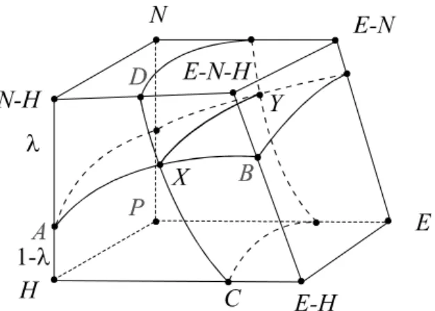
FIGURE 2. METHOD BY WHICH STREAMLINES ARE CONSTRUCTED FROM FIELD DATA.
DISCRETISATION SCHEME
The system of equations, Eq. (4), are suitable for discretisation using a finite-volume method (Patankar, 1980) resulting in sets of linear algebraic equations. Let it be assumed that the values of the velocity field are available at staggered locations. Field-values of ψ and θ may equivalently be computed at either cell centres or cell-corners (grid nodes). The latter were employed here, to facilitate graphical representation.
Suppose θ is temporarily known. The linear algebraic equations for ψ may be written as,
E E P W W P S S P N N P L L P H H P a - + a - + a - + a - a - + a - + S = ψ ψ ψ ψ ψ ψ ψ ψ ψ ψ ψ ψ ψ
1
6
1
6
1
6
1
6
+1
6
1
6
0 (7)where W, E, S, N, L, H refer to the West (i-1), East (i+1), South (j-1), North (j+1), Low (k-1), High (k+1) neighbours of node P. The linking coefficients are evaluated in terms of the metric components as W w a = Γg11 g
4
9
, E e a = Γg11 g4
9
etc., and the sub-scripts w, and e, refer to inter-nodal locations (i-½), (i+½). The volumetric source-term is,S g P g P g P g P g P g P w e n s h l ψ= − + − + − + 1 1 2 2 3 3
4
9 4
9 4
9
4
9 4
9 4
9
(8)where g is the grid Jacobian. When non-orthogonal
body-fitted grids are employed, an additional geometric source-term must be introduced into the equations to account for the influence of the diagonal neighbours, NE, SW, etc.
The resultant field of ψ-values are then used in the computations for S and Γ in the θ equations. Spalding’s whole-field solver (Spalding, 1981) which is a strongly implicit scheme was used to solve the system of linear algebraic equations.
Graphics utility
A procedure was written to plot streamlines corresponding to specific pair of values of ψ = ψ0 and θ = θ0, with reference to Fig. 2, as follows.
(i) Each cell was parsed to see if the eight corner values spanned both ψ = ψ0 and θ = θ0. (ii) The cell faces were in turn parsed to see if they spanned both ψ = ψ0 and θ = θ0. (iii) If so, the pairs on the face were parsed to see if they spanned either ψ = ψ0 or θ = θ0. The position of points A and B, corresponding to the intersection of the surface ψ = ψ0, with the cell perimeter were interpolated from the appropriate corner points, e.g.,
λ=
1
ψ0−ψH6 1
ψNH−ψH6
. Points C and D were similarlyobtained. (iv) The lines A-B and C-D were analysed to see if they intersect. (It is possible for a set of corners to span a pair of values, without the two surfaces intersecting each other). The point of intersection X of the two curves was then computed. (v) Steps (ii)-(iv) were repeated until a second point
Y found, and the curve X-Y drawn.
The process was repeated over the whole field for successive pairs of values (ψ,θ) over the entire range of values, resulting in a double-contour field.
EXAMPLES
Figure 3a shows a rectangular obstacle, placed in the path of a flow. Values of ψ and θ were prescribed at opposite sides of the domain. Figure 3b shows 3D streamlines around the obstacle corresponding to particular values of ψ and θ, as discussed above. Figure 3c illustrates vectors in the symmetry plane while in Figure 3d iso-values of θ in the symmetry plane are displayed. Due to symmetry, θ contours resemble 2D streamlines, passing around the rectangular block, with a pair of well-formed vortices occurring downstream in the wake.
Figure 4 shows a vortical flow above a plane, generated by prescribing the circulation at the top of the domain. Figure 4b illustrates streamlines for the problem at hand. It can be seen that the streamlines form well-defined closed loops, with the line-density increasing at higher levels due to the mass flow being greater.
DISCUSSION
The results show that two scalars, satisfying coupled diffusion-source equations, solved using a finite-volume method may be used to display streamlines which either enter or leave the finite-domain, or form closed curves in 3D.
The current method is based on the work of Beale (1993a,b) where the general purpose CFD code PHOENICS was used to solve diffusion-source equations, with Γ =1 . For the work, described here, original source code was developed in the C-language. The code contained two significant modifications: (a) Improvements in the numerical scheme were effected, (b) non-orthogonal source terms were introduced.
In the earlier work, numerical stability proved to be a matter for concern. The original form of the ψ-equation was for
P= −ρu& &× ∇ ∇ ⋅∇θ θ θ& & . When gradients were small, both
numerator and denominator simultaneously became small, leading to undesirable instabilities. By setting Γ = ∇ ⋅ ∇&θ θ& , the influence of neighbour-values is rendered negligible when gradients are small: Caution is still required when solving strongly-coupled systems of equations; and reasonable initial fields and boundary values must be selected for ψ and θ, however the overall stability of the algorithm has been substantially improved.
The second modification involves the addition of non-orthogonal terms to Eq. (5). Beale (1993a,b) considered only vorticity source terms. It is not always be possible to define stream functions, which are mutually orthogonal, ∇ ⋅∇ =&ψ θ& 0 and also satisfy the mass-flux condition, Eq. (2) (except for special circumstances, such as potential flow). The originally-defined orthogonal functions do satisfy Eqs. (1), i.e., are stream functions, and may therefore be used to construct streamlines and surfaces, for flows with re-circulation. However, the inclusion of the non-orthogonal terms in Eq. (5) is seen as a natural extension to the original methodology, ensuring that streamline density is proportional to the flow rate.
Kenwright and Mallinson (1992) also developed a strategy, based on the use of two stream functions. For global computations, their method is restricted to problems where ψ and θ satisfy an extremum principle, (Knight and Mallinson, 1996), i.e. there are no interior vortices. This approach is thus better suited to local streamline tracking, somewhat akin to Lagrangian particle tracking, but based on conservation principles.
In this author’s method, a finite-volume solver using a full 6-way elliptic solver was employed, and ψ and θ may exhibit local extrema, within the interior of the domain, without difficulty. Future work should address improvements in computational speed. Ideally a non-iterative marching algorithm, based on known upwind values of ψ and θ should be employed. However, if a solid surface (or surfaces), is selected to correspond to an iso-value of ψ, it may not be possible to specify a reference θ-surface, a priori. Thus some iteration may be unavoidable. But under many circumstances it would be advantageous to eliminate the influence of at least some of the linking-neighbours, aE , aN, aH and associated source terms, Pe, Pn, Ph, etc, in Eqs. (7) and (8), so as to expedite the solution
efficiently. As noted in Beale (1993a,b), there are many problems involving multiply-connected geometry’s, where it is desirable to keep active the influence of all 6 neighbours in the linear algebraic equations.
One advantage of using the ∇ψ& and ∇θ& directions is that the linking coefficients, thus generated, are guaranteed to be positive (Patankar, 1980). Equations based on the product of Eq. (2) with the co-ordinate directions, may also prove worthy of pursuit. The precise form of improved schemes, and how they may be generalised to apply to a variety of problems and geometry’s, is the subject of ongoing work. It is apparent that substantially more research is required in the area of stream-function generation, and in the subject of flow visualisation, in general.
CONCLUSIONS
A method for generating and plotting stream-surfaces and streamlines in three-dimensions has been described. The method involves the global solution for two scalar fields, ψ and
θ, governed by a pair of coupled partial differential equations. The specific approach employed involved the use of a finite-volume method, based on the numerical solution of Eqs. (4) and (5). This may be considered equivalent to the solution of Eqs. (3) using a finite-difference approximation. Any other numerical procedure, for example a finite-element analysis, may be readily employed to compute stream functions in a similar fashion.
Iso-values of ψ and θ may be used to plot stream-surfaces: Stream-lines are obtained as the locus of intersection of stream-surfaces. The entire flow may be illustrated as a double contour field over a range of values, ψmin≤ ≤ψ ψmaxand θmin≤ ≤θ θmax, the line density being proportional to the mass
flow rate. Because the scheme is conservative, vortices appear as simple closed loops, not as endless spirals. Existing Lagrangian methods require the judicious choice of reference points, in order to adequately describe the flow field. In the method described in the paper, fields of values of ψ and θ are known globally, and thus the user may rapidly obtain information about the entire flow field in an automatic manner.
ACKNOWLEDGEMENTS
The continuing support of the National Research Council is gratefully acknowledged. Original FORTRAN and GKS-based utilities, developed by the author while on professional leave at CHAM Ltd., in the summer of 1991, were ported to a C and GL-based environment with the assistance of Mr. Ron Jerome, to whom I am indebted.
REFERENCES
Beale, S.B., 1993a “Fluid Flow and Heat Transfer in Tube Banks”. PhD Thesis, Ch. 7 “Stream Functions”, University of London, pp. 121-131.
Beale, S.B. 1993b “A Numerical Scheme for the Generation of Streamlines in Three Dimensions”. Proc. 1st Ann. Conf. CFD Soc. Canada - CFD93, Montreal, June 14-15, pp. 289-300. Giese, J.H. 1951. “Stream Functions for Three-Dimensional Flows”, J. Math. Phys., Vol.30, pp. 31-35.
Kenwright, D.N. and Mallinson, G.D. 1992 “A 3-D Stream-line Tracking Alorithm using Dual Stream Functions”, Proc. Visualisation ’92, pp. 62-68, 19-23 Oct. 1992.
Kenwright, D.N., 1993. PhD Thesis, University of Aukland. Knight, D., and and Mallinson, G.D. 1996 “Visualising Unstructured Flow Data Using Dual Stream Functions” IEEE
Trans. Vis. Comput. Graphics. 2, 4, 1996.
Patankar, S.V. 1980. Numerical Heat Transfer and Fluid
Flow. Hemisphere, New York.
Rouse, H. Editor, Advanced Mechanics of Fluids. pp. 37-45. John Wiley, New York, 1959.
Sherif, A. Hafez, M. Int. J. Numer. Methods Fluids. 8, 17-29, 1988.
Spalding, D.B. 1980. “Mathematical Modelling of Fluid-mechanics, Heat-transfer and Chemical-reaction Processes: A Lecture Course”, HTS/80/1, Computational Fluid Dynamics Unit, Imperial College, University of London.
Wu, C-H. NACA TN 2605. 1952.
Yih, C.S. 1957. “Stream Functions in Three-dimensional Flows”. La Houille Blanche, No. 3, pp. 445-450.