The Augmented Geometrically Spaced Transform:
Applications of the Single Channel Frequency
Estimator
by
Jonathan Michael Feldman
B.Ed. University of Western Ontario (2004)
B.Sc. McGill University (1996)
Submitted to the Program in Media Arts and Sciences
School of Architecture and Planning
in partial fulfillment of the requirements for the degree of
Master of Science in Media Arts and Sciences
at the
MASSACHUSETTS INSTITUTE OF TECHNOLOGY
January 2021
© Massachusetts Institute of Technology 2021. All rights reserved.
Author . . . .
Program in Media Arts and Sciences
School of Architecture and Planning
February 2021
Certified by . . . .
Joseph A. Paradiso
Professor
Thesis Supervisor
Accepted by . . . .
Tod Machover
Academic Head
Program in Media Arts and Sciences
The Augmented Geometrically Spaced Transform:
Applications of the Single Channel Frequency Estimator
by
Jonathan Michael Feldman
Submitted to the Program in Media Arts and Sciences School of Architecture and Planning
on February 2021, in partial fulfillment of the requirements for the degree of
Master of Science in Media Arts and Sciences
Abstract
The Augmented Geometrically Spaced Transform (AGST) is an auditory model that is based on an inversion of the acoustic piano, where the piano produces music and the transform analyses it. In contrast with the standard spectrogram, which is a com-plex frequency vector versus time, the AGST is based around a matrix of frequencies, known as the AGST Frequency Matrix, where for every frequency in the matrix, a spectral envelope is computed using a Single Channel Frequency Estimator (SCFE). The core invention of the thesis is the algorithm for the SCFE, which computes spec-tral envelopes with maximally high definition in a computationally efficient manner. A bank of SCFEs is assembled into a constant Q transform, known as a
Geometri-cally Spaced Transform (GST). The GST can be used to visualize harmonics inside of
musical notes, or audio in general, in a constant Q fashion. It is then shown that the AGST is a good front-end model for computational pitch perception. For example, it can be used to solve an important problem in auditory perception, the case of the missing fundamental. The entire thesis is framed in the context of building artificially intelligent music systems, including synthetic listeners (machines that listen in the way that people do), and synthetic performers (machines that allow for interactive music performance).
Thesis Supervisor: Joseph A. Paradiso Title: Professor
Acknowledgments
I would like to thank many people for their encouragement and support in writing this thesis. First and foremost, I would like to thank my advisor Joe Paradiso, for supporting my research direction and helping me return to the lab in 2020 to complete my master’s thesis.. I would then like to thank my original thesis advisor, Barry Vercoe, for inviting me to join the Machine Listening Group at the Media Lab in 1996. Both Joe and Barry are visionaries in the world of audio, and I truly had no idea how much I would learn from both of them.
I would really like to thank my thesis readers, Bill Gardner and Spencer Russell. They have both offered valuable guidance, insight, and support toward the completion of this thesis. I would also like to thank everyone in the Responsive Environments
Group for making me feel welcome this term.
In my 4th year at McGill University, I discovered the field of auditory scene
anal-ysis, through the work of Dan Ellis. In a very coincidental way, I also discovered that
the father of auditory scene analysis, Dr. Albert Bregman, was in the psychology department at McGill. Along with a number of other students who were studying computer music with Bruce Pennycook in the music department, I took Dr. Breg-man’s course. The course was fascinating, I had never taken a psychology course before and Dr. Bregman’s work on auditory scene analysis amazed me. I was very lucky to have had a number of insightful and interesting conversations with him, and I enjoyed his course very much. I thank him with much respect because now I realize that he followed a scientific process in research related to auditory perception.
I would then like to give a special thanks to Dan Ellis. It was Dan’s work on
computational auditory scene analysis that I so admired that led me to apply to the
Media Lab. I am also indebted to Eric Scheirer, who was my office mate, whose work I also studied as a 4th year undergrad at McGill. While I was a student, I had many fruitful conversations with everyone in the group, including Paris Smaragdis, Michael Casey, Bill Gardner, Keith Martin, Adam Lindsay, and Joe Pompei, and they are all inspirations to my work. And a very warm and special thanks to Judy Brown, who
invented the Constant Q Transform. She was an associate of the Machine Listening
Group while I was a student and I had no idea that in the end, my research would
be based on her work.
I would like to thank all of my professors while I was a graduate student, in-cluding Michael Bove, Rosalind Picard, Michael Jordan, Neil Gershenfeld, Whitman Richards, Sherry Turkle, Mitch Resnick, and James Ward. A special thanks goes to Kay Shelemay, as I was lucky to be able to cross-register for a course in ethnomusi-cology at Harvard. It was this class that rounded out my Media Lab experience and balanced out my education between arts and sciences.
Another very important mentor of mine was Marvin Minsky. I was very curious about AI, and I was lucky to have a number of amazing conversations with him about AI and music. He was the person who warned me that trying to solve problems in AI and music are very hard. He was right, they are hard, but it has been a fun journey applying everything I know about math and music and ultimately developing a deeper understanding of artificial intelligence.
Yet another very important mentor of mine is Bob Chidlaw. From 1998-2000, I took a break in my studies at the Media Lab and worked at Kurzweil Music Systems where I conducted research on reverb algorithms, and he was the chief scientist there. Bob gave me an opportunity to get hands on experience in the music technology industry, and was the person who got me interested in the field of audio engineering. I would like to thank a number of people of other Media Lab students who were great friends while I was at MIT: Ben Vigoda, Kathi Blocher, Jocelyn Scheirer, Arjan Schutte, and Jon Dakks. I would also like to mention my close friend Aaron Lipman, and my other housemates Russell Epstein and Alex Holcombe.
I would like to thank all of my other teachers that I have had throughout my lifetime, who are like a converging Taylor series to me. They include my professors at McGill University, my high school teachers at Westdale High School, my elementary school teachers at the Hamilton Hebrew Academy, and the professors at both Western University where I studied education and at the University of Toronto where I studied music performance. Every teacher I have had in my life has had a huge impact
on me, as I always loved school and loved learning. It is truly a dream to look back and think of everyone who has taught me something, especially about math and music. One person I must mention is Russ Weil, who was the director of the music department at Westdale High. He gave me the opportunity to play in the Westdale jazz band, and ultimately the Hamilton All-Star Jazz Band. While I was classically trained in music from a very young age, my musical development really bIossomed when I fell in love with jazz. I’ve had many great piano teachers along with way outside of school, including Honey Burkle, Donna Barnes, Roland Packer, Bart Nameth, Tilden Webb, Yelena Neplokova, David Zoffer, Jerry Bergonzi, David Braid, and Gary Williamson. That said, I really do now love all of the disciplines and am grateful for all of the courses I have taken throughout my lifetime, and all of the wonderful teachers who taught them. All of that said, I would also like to mention a fantastic music teacher that I had when I was a student at U of T. Instead of strictly following the requirements in jazz performance, I took two music theory courses on classical music, that were taught by Mark Sallmen. He is the guy who dissected classical music theory for me and taught me advanced classical music ear training. Every now and again he would reference a pop or rock song, but for the most part he explained music in the tradition of Mozart, Beethoven, Haydn, Brahms, Tchaikovsky, and other great classical composers.
Finally, I would like to thank my family for all of their support and encouragement, including my father David, my mom Ilona, my sister Kayla, and Mark. Kayla is my closest, one and only sibling. Her work aesthetic and skills as a mom are an inspiration. My mom Ilona has been supportive of me in every way of my academic endeavors throughout my life, and for that I am truly grateful. Finally, all of my other aunts, uncles, and cousins, my brother-in-law, niece, and nephew, and my step-siblings and their families have been there for me as well, and I am truly blessed to have such a wonderful inclusive family.
This masters thesis has been examined by a Committee of the
Department of Media Arts and Sciences as follows:
Professor Joseph A. Paradiso . . . .
Chairman, Thesis Committee
Professor of Media Arts and Sciences
Dr. William G. Gardner . . . .
Thesis Supervisor
Ph.D., President, Wave Arts, Inc.
Dr. Spencer Russell . . . .
Member, Thesis Committee
Ph.D., Media Arts and Sciences
Contents
1 Introduction 17
2 A Brief History and Background 21 3 Time-Frequency Analysis 25
3.1 Introduction . . . 25
3.2 Constant Q Transform History . . . 29
3.3 Complex Exponentials . . . 30
3.4 Discrete Fourier Matrix . . . 31
3.5 Short-Time Fourier Transform . . . 32
4 Online Fourier Transform 35 4.1 Introduction . . . 35
4.2 Forward Algorithm . . . 37
4.2.1 Analysis . . . 40
4.3 Phase Update Method . . . 40
4.3.1 Forward Algorithm . . . 42
4.3.2 Inverse Algorithm . . . 43
5 Single Channel Frequency Estimation 47 5.1 Introduction . . . 47
5.2 Forward Algorithm . . . 47
5.2.1 Analysis . . . 48
5.2.3 Examples . . . 56
5.3 Inverse Algorithm . . . 58
6 Geometrically Spaced Transform 61 6.1 Introduction . . . 61
6.2 Forward Algorithm . . . 61
6.3 Calculation of Q . . . 66
6.4 Examples . . . 67
6.5 Inverse Algorithm . . . 69
7 Computational Pitch Perception 71 7.1 Augmented Geometrically Spaced Transform . . . 71
7.2 The Summed AGST . . . 73
7.3 Onset Detection . . . 75
7.4 Pitch Perception . . . 76
7.4.1 Pitch Tracking . . . 76
7.4.2 The Case of the Missing Fundamental . . . 79
7.5 Analysis and Future Work . . . 81
8 Conclusions 83 A Synthesis 87 A.1 Monophonic Synthesizer . . . 87
A.2 Polyphonic Synthesizer . . . 91
B Signal Reconstruction 93 C On Music and Technology 95
List of Figures
3-1 Pattern of Fourier Transform harmonic frequency components plotted
against log(frequency) . . . 26
3-2 Brown’s Constant Q Transform example . . . 27
3-3 GST analysis that mimics Brown’s example . . . 27
3-4 STFT analysis of piano note A110, N = 1024, hop = 1, 𝑓𝑠 = 48 kHz . 34 3-5 STFT analysis of piano note A110, N = 1024, hop = 256, 𝑓𝑠 = 48 kHz 34 4-1 A Fourier cylinder rolling across the input samples . . . 36
4-2 OFT Magnitude and Phase analysis of a 1 kHz sine tone . . . 41
4-3 OFT analysis of audio input of piano note A2 . . . 42
4-4 OFT phase update algorithm magnitude and phase analysis of a 1 kHz sine tone . . . 44
5-1 FIR filterbank which describes the SCFE rectangular summation . . . 49
5-2 Constant Q SCFE frequency response for 𝑓𝑘 = 0.5 kHz . . . 50
5-3 Constant Q SCFE frequency response for 𝑓𝑘 = 1 kHz . . . 50
5-4 Constant Q SCFE frequency response for 𝑓𝑘 = 2 kHz . . . 51
5-5 Constant Q SCFE frequency response for 𝑓𝑘 = 4 kHz . . . 51
5-6 Constant Q SCFE frequency response for 𝑓𝑘 = 8 kHz . . . 52
5-7 Constant Q SCFE frequency response for 𝑓𝑘 = 16 kHz . . . 52
5-8 SCFE frequency response at 5 kHz, N = 125 samples . . . 53
5-9 SCFE frequency response at 5 kHz, N = 250 samples . . . 53
5-10 SCFE frequency response at 5 kHz, N = 500 samples . . . 54
5-12 SCFE frequency response at 5 kHz, N = 2000 samples . . . 55
5-13 SCFE frequency response at 5 kHz, N = 4000 samples . . . 55
5-14 Harmonic analysis of A2 on the Piano . . . 56
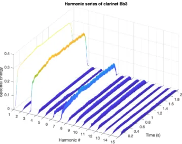
5-15 Harmonic analysis of Bb3 on the clarinet . . . 57
5-16 Harmonic analysis of A2 on the electric guitar . . . 57
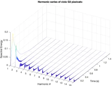
5-17 Harmonic analysis of G3 on the viola played pizzicato . . . 58
6-1 Signal flow diagram for GST algorithm . . . 63
6-2 Block lengths for GST algorithm . . . 64
6-3 Magnitude response of the GST filters for every note A on the piano . 64 6-4 Magnitude response of the 88 filters of the GST filterbank . . . 65
6-5 Magnitude responses of 16 gammatone filters in the frequency range 300-8000 Hz . . . 65
6-6 Q of each GST channel . . . 66
6-7 GST analysis of piano note A110 . . . 67
6-8 GST analysis of piano note A220 . . . 67
6-9 GST analysis of piano note A330 . . . 68
6-10 GST analysis of guitar note A110 . . . 68
6-11 GST analysis of bass trombone note A110 . . . 69
6-12 GST analysis of a tambourine slap . . . 69
7-1 AGST Frequency Matrix that extends from 3 Hz to 83720 Hz . . . . 72
7-2 AGST Frequency Matrix that shows which frequencies lie from 20 Hz to 20 kHz . . . 72
7-3 Snapshot of AGST of piano note A2 . . . 73
7-4 Snapshot of AGST of piano note C#3 . . . 74
7-5 Snapshot of AGST of piano note E3 . . . 74
7-6 Snapshot of AGST of piano note G3 . . . 75
7-7 Spectral envelope produced by the sum of the subharmonics . . . 76
7-8 Algorithm for pitch estimation . . . 77
7-10 Pitch estimation algorithm output for piano note A110 . . . 78 7-11 Summed AGST for major scale starting on A110 . . . 78 7-12 Pitch estimation algorithm output for major scale starting on A110 . 79 7-13 GST analysis of G196 synthesized with a missing fundamental . . . . 80 7-14 Summed AGST of G196 with missing fundamental with pitch perceived
as 196 Hz . . . 80 7-15 GST analysis of G196 synthesized with a missing lowest 4 harmonics 81 7-16 Summed AGST of G196 with missing lowest 4 harmonics with pitch
perceived as 196 Hz . . . 81 A-1 Signal flow diagram for SCFE synthesizer . . . 87 A-2 SCFE synthesizer i/o with quadratic based input function . . . 88 A-4 SCFE synthesizer with processed trombone sample using successive FFTs 89 A-3 SCFE synthesizer i/o with unusual real input . . . 89 A-5 Spectrogram of synthesizer output . . . 90 A-6 Polysynth output of a bank of 3 linear ramp input functions with
Chapter 1
Introduction
The Augmented Geometrically Spaced Transform is a K x M x N tensor that is a novel representation of a signal. There are K frequency channels, M harmonics, and N samples that are computed using Single Channel Frequency Estimators, or SCFEs. On the K axis it computes frequency envelopes and on the N axis it computes spectral envelopes. The M axis models a second order differential equation that computes harmonics. In the most general sense, the SCFE is a signal analysis tool that has a centre frequency 𝑓𝑘 and a setting for its Q. For the purpose of this thesis, I let
𝑄 = 16.81... since this corresponds to semi-tone spacing in music. But in practicality,
it can be tuned to any desired centre frequency 𝑓𝑘 and can be used with any Q you
choose. In the case of audio, with infinitely high oversampling, there is infinite time resolution at lower frequencies that lie in the frequency range of human hearing. It’s applications lie in the area of auditory signal analysis, including music, speech, bird songs, and other auditory-based recordings. It, however, can also be used to analyse sound that lies above the range of human hearing. For example, with high enough sample rates, the system could be used to analyse various bands of signals such as microwaves, x-rays, and ultrasound. This thesis is a scientific-based history of the discovery of this signal representation.
The applications are numerous and I hope that people will find this to be a useful tool in research. I have tried to show how it useful for analysing musical instrument samples, such as the piano and the electric guitar. I assume a basic understanding of
music, such as music theory in the tradition of Western musicology where the tonic, sub-dominant, and dominant chords play an essential role. Just like Darwin observed the Galapagos Islands and created a theory of evolution, I have observed my own musical development and my knowledge of both piano and guitar-based music that has influenced my musical knowledge and experience. While the experience of music is subjective, here I propose that it can be analysed using computational methods.
One important idea that I propose is that auditory perception is an evolution-ary process. People have been learning to listen to sounds for thousands of years, beginning perhaps with the weather, drumbeats that were used in tribal practices, drumbeats that were used for communication, and musical instruments that were tuned in various ways. Concerning music, the ear has learned to listen to music, including harmony. The psychological elements of auditory perception, including the perception of pitch, beats, and timbre, evolved over time. What the ear is able to listen to and enjoys listening to then continues to evolve through the creation of new musical instruments and new methods of playing them.
I suggest that there is a clear link between music, technology, and culture. Based on this observation and the theory developed here, I suggest that there is an emerging field of study known as computational ethnomusicology. It is the study of how com-putational methods can be used in anthropological research, especially as it relates to music in culture. By the end of the thesis, I will show how the Augmented GST can be used as an analysis tool to study music from any world culture. I will also suggest, however, that it may be biased towards music that stems from Western Civ-ilization, where for many centuries the piano has been the dominant compositional tool. I will also suggest that the ear has certain innate abilities to analyse the sound that enters the auditory system, but its interpretation and enjoyment is culturally subjective. The idea then, of computational ethnomusicology, is to have a compu-tational framework that can be used to study music, and I would also suggest that the model could be expanded, for instance, to be useful for listening to the music of India, where quarter-tone spacing is highly relevant to their form of classical music. The thesis then is quite open ended because now that I have written it, it is clear
that it leads to further work in physics, affective computing, artificial intelligence, computational modelling, robotics, and other disciplines including music theory and ethnomusicology.
Chapter 2
A Brief History and Background
The idea of synthetic performance was pioneered at M.I.T. in the 1980s, where Barry Vercoe built a music accompaniment system for a live flutist [Vercoe1984a] [Vercoe1984b]. The flute had to be augmented with optical sensors to aid the real-time pitch detection algorithm that was used to drive the system. Vercoe described computer-based accompaniment systems as systems that could listen, learn, and per-form with human musicians. This system motivates the need for real-time pitch detection algorithms. The work was also pursued at other music research institutes such as IRCAM where Pierre Boulez employed real-time computer interpretation of audio in enhanced live performances with his Ensemble Intercontemporain.
There are a number of algorithms that go together to build a machine that
lis-tens. These include pitch detection, beat tracking, tempo tracking, et al, potentially
including instrument identification and source separation. These auditory listening processes need to happen in real-time. Many algorithms that were developed by the
Machine Listening Group at the M.I.T. Media Lab and others in the 1990s, including
[Slaney1990], [Scheirer1997], [Martin1998], and [Smaragdis2001] are founda-tional to building real-time sophisticated synthetic performance systems. What is needed is a comprehensive auditory model that acts as a real-time front end proces-sor and is an integrated framework for computational auditory perception.
One potential application of such a model, as it applies to building synthetic per-formers, is interactive music performance, systems where humans and computers can
interact and perform music together. A dream system would be a system that aug-ments the experience of not just jamming and performing, but also aspects of learning to play music, such as practicing technique and ear training. In the end, it would be fun to play interactive musical games as Ben Vigoda describes in Musical Games:
A Guide for Group Improvisation, also known as Games for Song [Vigoda2005].
Playing these games are an example of meaningful musical group experiences. In order for synthetic musicians to truly be successful, the boundary between humans and machines would need to be blurred to a point where these machines pass the Turing test for creating music as art [Turing1950].
Other practical applications of having an accurate perceptual computational model of audition includes building more sophisticated hearing aids, music production sys-tems, and other AI-based sound and music processing tools.
In this thesis, I propose a computational model of pitch perception that is based on a matrix of frequency estimators that compute spectral envelopes called the
Aug-mented Geometrically Spaced Transform. I propose a constant Q frequency analyser,
called the Geometrically Spaced Transform (GST), as a computational alternative to typical front-end auditory modelling and processing such as the Patterson and Holdsworth auditory model [Patterson1995]. I then show that the GST can be augmented by computing a tensor based on what I call the AGST Frequency Matrix. This forms the basis of a computational model of pitch perception, and can be used as a real-time system that computes pitch and, for instance, solves an important problem in pitch perception, the case of the missing fundamental. I then show that the inverse SCFE can be used to synthesize monophonic audio and the inverse GST can be used to synthesize polyphonic audio.
In the original title of this thesis I used the term Online Frequency Estimation. I envisioned a system where frequency estimates are computed as every new sample enters the system. With this in mind, I had the idea that every frequency estimate could be computed using a linear update rule, and this would give the maximum time-frequency resolution possible. In Neil Gershenfeld’s The Nature of Mathematical
N-periodic. I envisioned spectral signal processing as having the Fourier matrix roll like a cylinder across the input samples. This is atypical in traditional discrete-time signal processing where spectral estimates are computed on blocks of input samples. However, the approach taken here is that the auditory system operates computationally in an online fashion and is high resolution, thus giving it high fidelity. Using this approach, and following the seminal papers written by Judith C. Brown [Brown1990] [Brown1992], I was able to derive an algorithm for online machine listening that is constant Q and wavelet-like where frequency estimates are more localized in time as frequency increases towards the top end of the hearing spectrum. I now frame the thesis in a larger context, and explain how it might be related to the field of Affective Computing [Picard1995]. I suggest that auditory perception is an evolutionary process, and that the perception of auditory elements in music such as pitch, beats, and timbre has changed over time. One goal of this may be to enhance the emotional experience of the listening process. For example, the more a person listens to music that is based on the rules of classical harmony and that is tuned based on the equal-tempered scale, the better it is able to enjoy a peaceful, harmonious listening experience [Haignere2013]. By harmonious, I mean an experience that produces emotions that excite the corresponding emotional patterns in the brain. I would suggest, for example, that Mozart played in major keys is more peaceful to listen to than the blues, rock music, or heavy metal. Music in general plays with the emotions in the brain, which is exemplified, for example, by the solo piano improvisations of Keith Jarrett. He has synthesized classical and jazz in a harmonious way that tells a story, that travels through the emotional experience of living life by using intricate, harmonic-based chord progressions. But I think from an emotional point of view, one way of ensuring a happy experience is to listen to music that is based on the chord progression of the tonic travelling to the sub-dominant travelling to the dominant and cadencing back to the tonic. This can be found for numerous examples in classical European music, traditional African music, rock n roll music such as Twist and Shout by The Beatles, ska music such as A Message To You Rudy by The Specials, reggae music such as Stir It Up by Bob Marley and the
Wailers, and electronic music such as Autobahn by Kraftwerk. What I mean to say is that every note and every chord in a musical sequence evokes emotion, and triggers corresponding emotion patterns in the brain that are a response to harmony. The emotional experience is a direct response to the harmonic experience.
I also believe that it is important to keep in mind that music has an anthropological significance. I am reminded of the thought that music creates culture and the idea that the music that people listen to triggers an emotional response that influences human thought, feeling, behaviour, and experience. For example, every generation in American culture since the advent of the blues in the early 20th century has given rise to dance, joy, sorrow, culture, and sociology. As music continues to evolve, society unfolds in new and myriad ways, as seen, for example, since the beginning of the 20th century where both musical and cultural development accelerated greatly, spurred by advances in recording, communications, and media technology. Culture and history continue to unfold in the 21𝑟𝑠𝑡 century as music, both new and old, is consumed
and experienced, where new culture emerges that is touched upon by the music that people listen to. These musical and cultural forces interact to create a diverse fabric of the human experience. It turns out that even cultural aspects of music performance, such as instrument choice, modes, and tunings, can be analysed with computational methods using a model such as the Augmented Geometrically Spaced Transform.
Chapter 3
Time-Frequency Analysis
3.1
Introduction
Time-Frequency Analysis is often used to compute a Spectrogram that displays fea-tures of a signal with time along the x-axis and frequency along the y-axis. Typical applications include music, sonar, radar and speech. The most common tool used to compute a Spectrogram is the Short-Time Fourier Transform (STFT), which uses the Fast Fourier Transform (FFT) to compute a frequency vector for each windowed block of the input signal. In the case of music and speech, where the contents of the signal contain pitched information, a logarithmic scale is typically used to display frequency. For music and speech analysis, the problem is that there is too little in-formation available at low frequencies and too much inin-formation at high frequencies. See figure (3-1). The result is that the Q of each frequency channel is wider at low frequencies and narrower at high frequencies.
𝑄 = 𝑓𝑘
Δ𝑓𝑘
(3.1)
The Constant Q Transform (CQT) was proposed to solve this problem [Brown1990]. See figure (3-2). Brown devises a 24 band per octave filter bank, which has quarter-tone spacing, and can resolve the fundamental frequencies of adjacent musical notes with a semitone spacing. Brown states that "the resolution should be geometrically
Figure 3-1: Pattern of Fourier Transform harmonic frequency components plotted against log(frequency)
related to the frequency e.g., 3% of the frequency in order to distinguish between fre-quencies with semitone (6%) spacing." What is desired is the ratio of centre frequency to bandwidth should be constant; that is, the Q factor of each frequency channel is constant.
I propose an alternative to this approach, which I call the Geometrically Spaced
Transform (GST), which uses a bank of Single Channel Frequency Estimators (SCFEs)
that are tunable to any desired center frequency. I tune the center frequencies to the fundamental frequencies of the notes of the piano, which are semi-tone spaced, and with the Q set as in equation (3.2):
𝑄 = 1
2121 − 1
(3.2)
In this thesis, the algorithm operates off-line. The algorithm is designed however to operate in an online fashion, where each successive filter output is computed using a linear update rule based on the previous filter output as each sample enters the system. Also note that here I suggest that semi-tone spacing is sufficient to resolve
Figure 3-2: Brown’s Constant Q Transform example
individual pitches and that quarter-tone spacing is not necessary as Brown suggests in [Brown1990]. See figure(3-3) where the GST mimics Brown’s figure.
Figure 3-3: GST analysis that mimics Brown’s example
Each SCFE is fast. It requires one real multiply, two real additions, two complex multiplies, and two complex additions to process each time domain sample. The
SCFE can be inverted to recover the original audio with perfect signal reconstruction to recover the audio input. In this thesis, I apply a matrix of SCFEs, known as the Augmented GST, and suggest that it can be used as a general auditory model for computational audition. Here, I focus on the CQS as the front end of a pitch detection system. In the end, I also show that the inverse SCFE algorithm can be modified to be used as a monophonic synthesizer, and the inverse GST algorithm can be modified to be used as a polyphonic synthesizer.
I further describe the Single Channel Frequency Estimator. Given a real-valued signal input, the algorithm estimates spectral energy at a given center frequency with a fixed Q. A typical use of this in music signal analysis is that the Q is fixed to resolve semi-tones of notes that are produced by typical Western musical instruments (𝑄 ≈ 17) [Mathieu1997]. A bank of SCFEs can be put together into a transform that mimics Brown’s Constant Q Transform (CQT), which I call the Geometrically
Spaced Transform.
I show a history of how I came to develop the SFCE algorithm, which begins with an observation about the periodic nature of the Discrete Fourier Matrix. I develop what I call the Online Fourier Transform, which is similar in principle to a
Short-Time Fourier Transform with a step size of one sample. I then show how instead of
computing this in matrix form, an algorithm can be developed by keeping track of phase as a phasor circulates around the complex unit circle. This leads to the formu-lation of the Geometrically Spaced Transform, where instead of computing linearly spaced frequency components, the computed frequency components are geometrically spaced, akin to the fundamental frequencies of the piano. The GST then is extended to formulate the Augmented GST, where an additional dimension is added to the GST to compute harmonics. It is this signal representation that is proposed as a computational auditory model and when it comes to computing pitch, it for example solves the problem of the missing fundamental [Moore1994].
3.2
Constant Q Transform History
The Constant Q Transform (CQT), which has geometrically spaced frequency chan-nels, was originally proposed by Brown in 1990 [Brown1990]. A more efficient implementation of the CQT was proposed in 1992 [Brown1992], which efficiently implements the following equation:
𝑋[𝑘] =
𝑁𝑘−1
∑︁
𝑛=0
𝑤[𝑛, 𝑘]𝑥[𝑛]𝑒−𝑗𝜔𝑘𝑛 (3.3)
While the CQT can be used for analysis purposes, a goal is to be able to in-vert the transform so that it can be used for re-synthesis. An approximate of an inverse transform was described by FitzGerald, Cranitch, and Cychowski in 2006 [Fitzgerald2006]. In 2010, an improvement on the inverse transform was proposed by Schorbuber and Klapuri who reported a signal-to-noise ratio of 55 dB for a re-synthesized input signal by analysing 12 bins per octave [Schorbuber2010].
A modified constant Q spectrogram was proposed by [Ingle2011], whose algorithm "computes the 𝑁𝑘-long DFT for each frequency, 𝑓𝑘, of interest and then picking out
the 𝑄𝑡ℎ DFT coefficient. The equation is as follows:
𝑋[𝑘] = 1 𝑁𝑘 𝑁𝑘−1 ∑︁ 𝑛=0 𝑤[𝑘, 𝑛]𝑥[𝑛]𝑒 −𝑗2𝜋𝑄𝑛 𝑁𝑘 (3.4)
The proposed Online Fourier Transform is similar to the Sliding DFT (SDFT) [Jacobsen2003]. The main difference between the two algorithms is that the SDFT uses a circular buffer whereas the OFT uses a circular matrix, which I call the Fourier cylinder. The result is that while the magnitude spectra are equivalent, the phase spectra are different. In the case of the SDFT, Jacobsen’s research lead to a con-stant Q transform, which is described in Sliding with a Concon-stant Q [Bradford2008]. Here, the OFT, via the phase update method, leads to the GST. The value of the GST compared to existing work is in its simplicity, compared with [Brown1992], [Bradford2008], and [Velasco2011].
3.3
Complex Exponentials
Complex exponentials are the basic unit that is used in harmonic analysis and can be found in both physics and electrical engineering. The complex exponential can be derived by solving the following differential equation:
𝑑𝑦
𝑑𝜃 − 𝑗𝑦 = 0 (3.5)
or
𝑑𝑦
𝑑𝜃 = 𝑗𝑦 (3.6)
The solution to (3.6) is the complex sinusoid
𝑦 = 𝑐𝑜𝑠𝜃 + 𝑗𝑠𝑖𝑛𝜃 (3.7)
Here note that
𝑑𝑦 𝑑𝜃 = −𝑠𝑖𝑛𝜃 + 𝑗𝑐𝑜𝑠𝜃 (3.8) and 𝑗𝑦 = −𝑠𝑖𝑛𝜃 + 𝑗𝑐𝑜𝑠𝜃 (3.9) So 𝑑𝑦 𝑑𝜃 = 𝑗𝑦 (3.10) and 𝑦 = 𝑐𝑜𝑠𝜃 + 𝑗𝑠𝑖𝑛𝜃 (3.11) is the solution.
I now examine the Taylor series for 𝑦 = 𝑠𝑖𝑛𝜃 and 𝑦 = 𝑐𝑜𝑠𝜃 and show that when I put them together according to
I get the Taylor series for 𝑦 = 𝑒𝑗𝜃. 𝑐𝑜𝑠𝜃 = 1 − 1 2!𝜃 2+ 1 4!𝜃 4− 1 6!𝜃 6+ 1 8!𝜃 8− ... (3.13) 𝑠𝑖𝑛𝜃 = 𝜃 − 1 3!𝜃 3 + 1 5!𝜃 5− 1 7!𝜃 7 + ... (3.14) So [1 − 1 2!𝜃 2+ 1 4!𝜃 4− 1 6!𝜃 6 + ...] + 𝑗[𝜃 − 1 3!𝜃 3+ 1 5!𝜃 5− 1 7!𝜃 7+ ...] (3.15) 1 + 𝑗𝜃 − 1 2!𝜃 2− 𝑗1 3!𝜃 3+ 1 4!𝜃 4+ 𝑗1 5!𝜃 5 − 1 6!𝜃 6− 𝑗 1 7!𝜃 7+ 1 8!𝜃 8+ ... (3.16) = 𝑒𝑗𝜃 (3.17) So 𝑒𝑗𝜃 = 𝑐𝑜𝑠𝜃 + 𝑗𝑠𝑖𝑛𝜃 (3.18) which is known as Euler’s Formula [Strang2014]
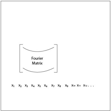
In this thesis, I begin by examining the Discrete Fourier Matrix, which is a ma-trix of complex exponentials. I use these complex exponentials to derive the Single
Channel Frequency Estimator, which forms the basis for the proposed Geometrically Spaced Transform and Constant Q Spectrogram.
3.4
Discrete Fourier Matrix
𝐹 = ⎡ ⎢ ⎢ ⎢ ⎢ ⎢ ⎢ ⎢ ⎢ ⎢ ⎢ ⎢ ⎢ ⎢ ⎢ ⎢ ⎣ 1 1 1 1 . . . 1 1 𝑤 𝑤2 𝑤3 . . . 𝑤𝑁 −1 1 𝑤2 𝑤4 𝑤6 . . . 𝑤2(𝑁 −1) 1 𝑤3 𝑤6 𝑤9 . . . 𝑤3(𝑁 −1 .. . ... ... ... . .. ... 1 𝑤2(𝑁 −1) 𝑤3(𝑁 −1) 𝑤6(𝑁 −1) . . . 𝑤(𝑁 −1)(𝑁 −1) ⎤ ⎥ ⎥ ⎥ ⎥ ⎥ ⎥ ⎥ ⎥ ⎥ ⎥ ⎥ ⎥ ⎥ ⎥ ⎥ ⎦ (3.19) where 𝑤 = 𝑒−𝑗2𝜋/𝑁 [Strang1998]
A Discrete Fourier Transform, calculated as a matrix multiplication, is as follows:
𝑋 = 𝐹 𝑥 (3.20)
Typically, however, the Fast Fourier Transform algorithm is employed instead of using matrix multiplication. An FFT efficiently computes such transformations by factorizing the DFT matrix into a product of sparse, mostly zero, factors. This reduces the computational cost from 𝑂(𝑁2) to 𝑂(𝑁 𝑙𝑜𝑔𝑁 ) [VanLoan1992]
3.5
Short-Time Fourier Transform
Given that I am trying to compute a new frequency estimate for every sample that enters the system, I examine the Short-Time Fourier Transform with a step size of one sample. Computing it this way ensures that the time resolution of the spectral output is maximal. Typically, with the STFT, a window is used, but here I show that for this algorithm windowing is not necessary. The Discrete Fourier Matrix is used at every step to calculate the Discrete Fourier Transform of the windowed input samples at any time t, and this is computed quickly using the Fast Fourier Transform algorithm [Cooley1965], which takes advantage of the structure of the Discrete Fourier Matrix to reduce the computation from a computational cost of 𝑂(𝑁2) to 𝑂(𝑁 𝑙𝑜𝑔𝑁 ) using
a recursive divide-and-conquer butterfly algorithm.
The standard method of then computing the Short-Time Fourier Transform ac-cording to [Smith2011] is:
𝑋𝑚(𝜔) =
∞ ∑︁
𝑛=−∞
𝑥(𝑛)𝑤(𝑛 − 𝑚𝑅)𝑒−𝑗𝜔𝑛 (3.21)
I simplify the math by showing how the DFT matrix can be used to compute an STFT in the N = 4 case. Note that everyone uses the FFT to compute an STFT, but here I am doing it with matrix multiplication because it informs the work to come on the Online Fourier Transform.
𝐹 = ⎡ ⎢ ⎢ ⎢ ⎢ ⎢ ⎢ ⎢ ⎢ ⎣ 1 1 1 1 1 −𝑗 −1 𝑗 1 −1 1 −1 1 𝑗 −1 −𝑗 ⎤ ⎥ ⎥ ⎥ ⎥ ⎥ ⎥ ⎥ ⎥ ⎦ (3.22) ⃗ 𝑥 = [︂ 𝑥1 𝑥2 𝑥3 𝑥4 𝑥5 𝑥6. . . ]︂ (3.23) The output of the STFT produces a spectrogram as follows:
⎡ ⎢ ⎢ ⎢ ⎢ ⎢ ⎢ ⎢ ⎢ ⎣ 1 1 1 1 1 −𝑗 −1 𝑗 1 −1 1 −1 1 𝑗 −1 −𝑗 ⎤ ⎥ ⎥ ⎥ ⎥ ⎥ ⎥ ⎥ ⎥ ⎦ ⎡ ⎢ ⎢ ⎢ ⎢ ⎢ ⎢ ⎢ ⎢ ⎣ 𝑥1 𝑥2 𝑥3 𝑥4 . . . 𝑥2 𝑥3 𝑥4 𝑥5 . . . 𝑥3 𝑥4 𝑥5 𝑥6 . . . 𝑥4 𝑥5 𝑥6 𝑥7 . . . ⎤ ⎥ ⎥ ⎥ ⎥ ⎥ ⎥ ⎥ ⎥ ⎦ = ⎡ ⎢ ⎢ ⎢ ⎢ ⎢ ⎣ .. . ... ... ... · · · ⃗ 𝑓4 𝑓⃗5 𝑓⃗6 𝑓⃗7 · · · .. . ... ... ... · · · ⎤ ⎥ ⎥ ⎥ ⎥ ⎥ ⎦ (3.24)
Note that in the STFT representation, the harmonics of the musical audio signal do not necessarily coincide with the centre frequencies of the bands that are being analysed. This is the motivation behind designing a geometrically spaced transform whose analysis frequencies match those of the typical frequencies inside of a harmonic-based sound. See figures (3-4) and (3-5) as examples of STFT-harmonic-based analysis of a piano note. Note that with the STFT, it is typical to use a window on the input samples before taking the FFT, which reduces spectral leakage between adjacent frequency channels.
Figure 3-4: STFT analysis of piano note A110, N = 1024, hop = 1, 𝑓𝑠 = 48 kHz
Chapter 4
Online Fourier Transform
4.1
Introduction
In this chapter, I discuss the Online Fourier Transform (OFT). I modify the STFT by making the observation that the DFT matrix is N-periodic. I derive a linear update rule to compute the filterbank output at each time step as a function of the previous timestep. In the end, I will have a time-frequency matrix, or spectrogram, where each frequency bin in a frequency estimate has been integrated over a time smear of N samples, but where otherwise, the representation has the maximum time resolution possible. I can show graphically, without a proof, that the magnitude of the OFT spectrogram is equal to the magnitude of the STFT spectrogram. The phase of the OFT differs however from the phase of the STFT because the OFT is demodulated. It appears that for spectral channels that exactly detect a sinusoid whose frequency is matched with the center frequency of its listening channel, the phase is a constant. Figure (4-1) shows how I envision the Fourier matrix rolling like a cylinder across the input samples. The mathematics in this section is similar to the Sliding DFT [Jacobsen2003] (shown below).
I now show the calculation of the OFT. Again, I simplify the math by showing the case for N = 4, i.e. where the DFT matrix is of size 4x4:
Figure 4-1: A Fourier cylinder rolling across the input samples 𝐹 = ⎡ ⎢ ⎢ ⎢ ⎢ ⎢ ⎢ ⎢ ⎢ ⎣ 1 1 1 1 1 −𝑗 −1 𝑗 1 −1 1 −1 1 𝑗 −1 −𝑗 ⎤ ⎥ ⎥ ⎥ ⎥ ⎥ ⎥ ⎥ ⎥ ⎦ 𝑥 = ⎡ ⎢ ⎢ ⎢ ⎢ ⎢ ⎢ ⎢ ⎢ ⎣ 𝑥1 𝑥2 𝑥3 𝑥4 ⎤ ⎥ ⎥ ⎥ ⎥ ⎥ ⎥ ⎥ ⎥ ⎦ (4.1)
Recall that a Discrete Fourier Transform is calculated as a matrix multiplication as 𝑋 = 𝐹 𝑥. Analysed in another way, the Discrete Fourier Transform is the vector projection of the input signal onto each row of the Discrete Fourier Matrix:
⃗ 𝑝1 = [︂ 1 1 1 1 ]︂ ⎡ ⎢ ⎢ ⎢ ⎢ ⎢ ⎢ ⎢ ⎢ ⎣ 𝑥1 𝑥2 𝑥3 𝑥4 ⎤ ⎥ ⎥ ⎥ ⎥ ⎥ ⎥ ⎥ ⎥ ⎦ ⃗ 𝑝2 = [︂ 1 −𝑗 −1 𝑗 ]︂ ⎡ ⎢ ⎢ ⎢ ⎢ ⎢ ⎢ ⎢ ⎢ ⎣ 𝑥1 𝑥2 𝑥3 𝑥4 ⎤ ⎥ ⎥ ⎥ ⎥ ⎥ ⎥ ⎥ ⎥ ⎦ (4.2) etc.
Using the idea of the Fourier Cylinder, each row of F can be seen as a complex wave (i.e. a complex exponential) and each row can be expanded cyclically:
⃗ 𝑝1 = [︂ 1 1 1 1 1 1 1 1 . . . ]︂ (4.3) ⃗ 𝑝2 = [︂ 1 −𝑗 −1 𝑗 1 −𝑗 −1 𝑗 . . . ]︂ (4.4) ⃗ 𝑝3 = [︂ 1 −1 1 −1 1 −1 1 −1 . . . ]︂ (4.5) ⃗ 𝑝4 = [︂ 1 𝑗 −1 −𝑗 1 𝑗 −1 −𝑗 . . . ]︂ (4.6)
4.2
Forward Algorithm
The DFT matrix is viewed like a cylinder moving across a real time input vector ⃗𝑥.
The notation is as follows. I use the matrix 𝐹4 to calculate a frequency estimate at
time t = 4 with input samples 𝑥1, 𝑥2, 𝑥3, and 𝑥4. Then at t = 5, I use 𝐹5 with input
𝐹4+𝑘𝑁 = ⎡ ⎢ ⎢ ⎢ ⎢ ⎢ ⎢ ⎢ ⎢ ⎣ 1 1 1 1 1 −𝑗 −1 𝑗 1 −1 1 −1 1 𝑗 −1 −𝑗 ⎤ ⎥ ⎥ ⎥ ⎥ ⎥ ⎥ ⎥ ⎥ ⎦ 𝐹5+𝑘𝑁 = ⎡ ⎢ ⎢ ⎢ ⎢ ⎢ ⎢ ⎢ ⎢ ⎣ 1 1 1 1 −𝑗 −1 𝑗 1 −1 1 −1 1 𝑗 −1 −𝑗 1 ⎤ ⎥ ⎥ ⎥ ⎥ ⎥ ⎥ ⎥ ⎥ ⎦ (4.7) 𝐹6+𝑘𝑁 = ⎡ ⎢ ⎢ ⎢ ⎢ ⎢ ⎢ ⎢ ⎢ ⎣ 1 1 1 1 −1 𝑗 1 −𝑗 1 −1 1 −1 −1 −𝑗 1 𝑗 ⎤ ⎥ ⎥ ⎥ ⎥ ⎥ ⎥ ⎥ ⎥ ⎦ 𝐹7+𝑘𝑁 = ⎡ ⎢ ⎢ ⎢ ⎢ ⎢ ⎢ ⎢ ⎢ ⎣ 1 1 1 1 𝑗 1 −𝑗 −1 −1 1 1 1 −𝑗 1 𝑗 −1 ⎤ ⎥ ⎥ ⎥ ⎥ ⎥ ⎥ ⎥ ⎥ ⎦ (4.8) ⃗ 𝑥 = [︂ 𝑥1 𝑥2 𝑥3 𝑥4 𝑥5 𝑥6. . . ]︂ (4.9)
To compute the next frequency estimate, the idea is given by:
⎡ ⎢ ⎢ ⎢ ⎢ ⎢ ⎢ ⎢ ⎢ ⎣ 1 1 1 1 1 1 . . . 1 −𝑗 −1 𝑗 1 −𝑗 . . . 1 −1 1 −1 1 −1 . . . 1 𝑗 −1 −𝑗 1 𝑗 . . . ⎤ ⎥ ⎥ ⎥ ⎥ ⎥ ⎥ ⎥ ⎥ ⎦ ⎡ ⎢ ⎢ ⎢ ⎢ ⎢ ⎢ ⎢ ⎢ ⎢ ⎢ ⎢ ⎢ ⎢ ⎢ ⎢ ⎢ ⎢ ⎢ ⎢ ⎣ 𝑥1 𝑥2 𝑥3 𝑥4 𝑥5 𝑥6 .. . ⎤ ⎥ ⎥ ⎥ ⎥ ⎥ ⎥ ⎥ ⎥ ⎥ ⎥ ⎥ ⎥ ⎥ ⎥ ⎥ ⎥ ⎥ ⎥ ⎥ ⎦ = ⎡ ⎢ ⎢ ⎢ ⎢ ⎢ ⎣ .. . ... ... · · · ⃗ 𝑓4 𝑓⃗5 𝑓⃗6 · · · .. . ... ... · · · ⎤ ⎥ ⎥ ⎥ ⎥ ⎥ ⎦ (4.10) where ⃗ 𝑓4 = ⎡ ⎢ ⎢ ⎢ ⎢ ⎢ ⎢ ⎢ ⎢ ⎣ 1 1 1 1 ⎤ ⎥ ⎥ ⎥ ⎥ ⎥ ⎥ ⎥ ⎥ ⎦ 𝑥1 + ⎡ ⎢ ⎢ ⎢ ⎢ ⎢ ⎢ ⎢ ⎢ ⎣ 1 −𝑗 −1 𝑗 ⎤ ⎥ ⎥ ⎥ ⎥ ⎥ ⎥ ⎥ ⎥ ⎦ 𝑥2+ ⎡ ⎢ ⎢ ⎢ ⎢ ⎢ ⎢ ⎢ ⎢ ⎣ 1 −1 1 −1 ⎤ ⎥ ⎥ ⎥ ⎥ ⎥ ⎥ ⎥ ⎥ ⎦ 𝑥3+ ⎡ ⎢ ⎢ ⎢ ⎢ ⎢ ⎢ ⎢ ⎢ ⎣ 1 𝑗 −1 −𝑗 ⎤ ⎥ ⎥ ⎥ ⎥ ⎥ ⎥ ⎥ ⎥ ⎦ 𝑥4 (4.11)
⃗ 𝑓5 = ⎡ ⎢ ⎢ ⎢ ⎢ ⎢ ⎢ ⎢ ⎢ ⎣ 1 −𝑗 −1 𝑗 ⎤ ⎥ ⎥ ⎥ ⎥ ⎥ ⎥ ⎥ ⎥ ⎦ 𝑥2+ ⎡ ⎢ ⎢ ⎢ ⎢ ⎢ ⎢ ⎢ ⎢ ⎣ 1 −1 1 −1 ⎤ ⎥ ⎥ ⎥ ⎥ ⎥ ⎥ ⎥ ⎥ ⎦ 𝑥3+ ⎡ ⎢ ⎢ ⎢ ⎢ ⎢ ⎢ ⎢ ⎢ ⎣ 1 𝑗 −1 −𝑗 ⎤ ⎥ ⎥ ⎥ ⎥ ⎥ ⎥ ⎥ ⎥ ⎦ 𝑥4+ ⎡ ⎢ ⎢ ⎢ ⎢ ⎢ ⎢ ⎢ ⎢ ⎣ 1 1 1 1 ⎤ ⎥ ⎥ ⎥ ⎥ ⎥ ⎥ ⎥ ⎥ ⎦ 𝑥5 (4.12) = 𝑓⃗4+ ⎡ ⎢ ⎢ ⎢ ⎢ ⎢ ⎢ ⎢ ⎢ ⎣ 1 1 1 1 ⎤ ⎥ ⎥ ⎥ ⎥ ⎥ ⎥ ⎥ ⎥ ⎦ 𝑥5 − ⎡ ⎢ ⎢ ⎢ ⎢ ⎢ ⎢ ⎢ ⎢ ⎣ 1 1 1 1 ⎤ ⎥ ⎥ ⎥ ⎥ ⎥ ⎥ ⎥ ⎥ ⎦ 𝑥1 (4.13) = 𝑓⃗4+ ⎡ ⎢ ⎢ ⎢ ⎢ ⎢ ⎢ ⎢ ⎢ ⎣ 1 1 1 1 ⎤ ⎥ ⎥ ⎥ ⎥ ⎥ ⎥ ⎥ ⎥ ⎦ (𝑥5− 𝑥1) (4.14) = 𝑓⃗4+ 𝐹:,1(𝑥5− 𝑥1) (4.15) So in general: ⃗ 𝑓𝑡 = ⃗𝑓𝑡−1+ 𝐹:,𝑡%𝑁(𝑥𝑡− 𝑥𝑡−𝑁) (4.16)
where the Fourier matrix F is expressed with Matlab indexing and is of size NxN and t%N is actually mod(t,N) if t <N and N if t = N. In the next section I use this equation to generate the Fourier coefficients of 𝐹:,𝑡%𝑁 on the fly. This method
leads to the GST. Note that the computational cost of a new frequency estimate in O(N) whereas the cost of computing an FFT is O(NlogN). This is of comparable computational complexity to the Sliding DFT [Jacobsen2003]:
𝑆𝑘,𝑡 = 𝑆𝑘,𝑡−1𝑒𝑗2𝜋𝑘/𝑁+ 𝑥𝑡− 𝑥𝑡−𝑁 (4.17)
Note that I am circulating the columns of the Discrete Fourier Matrix and whereas in the Sliding DFT, Jacobsen is using a fixed DFT matrix and a circular buffer for the samples according to the DFT circular shift property. Equations (4.16) and (4.17) differ by a modulation, according to the following equation:
𝑓𝑘,𝑡 = 𝑒
−𝑗2𝜋𝑘𝑡
𝑁 𝑆
𝑘,𝑡 (4.18)
4.2.1
Analysis
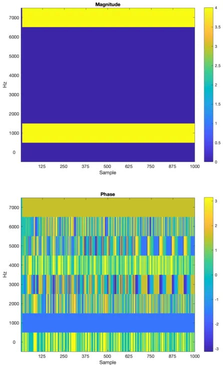
I begin by analysing a signal that contains a sine wave at 1000 Hz, with a sample rate of 8000 Hz. I set N = 8 so that the frequency channels are tuned to multiples of 1000 Hz, which results in 8 computed frequency channels. See figure(4-2).
In the magnitude response, the 1000 Hz band and corresponding imaginary 7000 Hz band are constant. Note that in the phase response, the band at 1000 Hz is constant at -𝜋/2 and the band at 7000 Hz is constant at 𝜋/2.
Because I am interested in analysing audio signals that contain music, I test the algorithm on a piano note whose fundamental frequency is 110 Hz. Here, the sample rate is 48 kHz. I display the first 64 channels. See figure (4-3).
Note that the harmonics of the piano notes are not well resolved in the magnitude response, with the low frequency information muddled together in the bottom few rows of the spectrogram. Note also, that in the phase response, there are horizontal bands that appear as features of the image. It appears that there is harmonic structure of the input signal that is being displayed by phase response.
4.3
Phase Update Method
In the previous section, I used the Discrete Fourier Matrix and let it roll like a cylinder across the input samples. I use one column of the matrix to compute each new frequency estimate. Here, instead of using the DFT matrix, I generate the Fourier coefficients on the fly. One advantage here is that I am able to derive a method to invert the transform. I can consider each frequency channel separately.
Figure 4-3: OFT analysis of audio input of piano note A2
4.3.1
Forward Algorithm
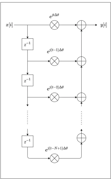
I define x to be the input signal, 𝑓𝑠to be the sample rate, N to be the window length
(integration constant), and M to be the number of frequency channels starting at DC. I consider frequency channel k at time t.
Initialization
I start with 𝑓𝑘,1= 𝑒𝑗0𝑥1 = 𝑥1 and then for t = 2:N
𝜃𝑘,𝑡 = 𝜃𝑘,𝑡+ Δ𝜃𝑘 (4.19)
𝑓𝑘,𝑡 = 𝑓𝑘,𝑡+ 𝑒𝑗𝜃𝑘,𝑡𝑥𝑡 (4.20)
I now have frequency estimates for the first N samples including the first complete N-point frequency estimate at time N ⃗𝑓𝑁.
Runtime
Starting with sample t = N+1:
𝜃𝑘,𝑡 = 𝜃𝑘,𝑡+ Δ𝜃𝑘 (4.21)
𝑓𝑘,𝑡 = 𝑓𝑘,𝑡−1+ 𝑒𝑗𝜃𝑘,𝑡(𝑥𝑡− 𝑥𝑡−𝑁) (4.22)
See figure (4-4) for an example of using the OFT with the phase update method.
4.3.2
Inverse Algorithm
I use the buffered first N samples to begin the output signal.
Then starting at time t = N+1:
I start with
Figure 4-4: OFT phase update algorithm magnitude and phase analysis of a 1 kHz sine tone
Expressed in vector form: ⃗ 𝑓𝑡 = ⃗𝑓𝑡−1+ 𝑒𝑗 ⃗𝜃𝑡(𝑥𝑡− 𝑥𝑡−𝑁) (4.24) ⃗ 𝑓𝑡 = ⃗𝑓𝑡−1+ 𝑒𝑗 ⃗𝜃𝑡𝑥𝑡− 𝑒𝑗 ⃗𝜃𝑡𝑥𝑡−𝑁 (4.25) ⃗ 𝑓𝑡− ⃗𝑓𝑡−1+ 𝑒𝑗 ⃗𝜃𝑡𝑥𝑡−𝑁 = 𝑒𝑗 ⃗𝜃𝑡𝑥𝑡 (4.26) I let ⃗ 𝑔𝑡= ⃗𝑓𝑡− ⃗𝑓𝑡−1+ 𝑒𝑗 ⃗𝜃𝑡𝑥𝑡−𝑁 (4.27) so I have ⃗ 𝑔𝑡 = 𝑒𝑗 ⃗𝜃𝑡𝑥𝑡 (4.28) Solving for 𝑥𝑡 𝑒𝑗 ⃗𝜃𝑡𝑥 𝑡 = ⃗𝑔𝑡 (4.29) 1 𝐾𝑒 𝑗 ⃗𝜃𝑡*𝑇𝑒𝑗 ⃗𝜃𝑡𝑥 𝑡 = 1 𝐾𝑒 𝑗 ⃗𝜃𝑡*𝑇𝑔⃗ 𝑡 (4.30) 𝑥𝑡 = 1 𝐾𝑒 𝑗 ⃗𝜃𝑡*𝑇(⃗𝑓 𝑡− ⃗𝑓𝑡−1+ 𝑒𝑗 ⃗𝜃𝑡𝑥𝑡−𝑁) (4.31)
Chapter 5
Single Channel Frequency
Estimation
5.1
Introduction
An SCFE is a high definition recursive digital filter. Each SCFE has a center frequency
𝑓 , a 𝑄, and an integration length 𝑁 that determines the number of samples over which
a frequency estimate is summed. Note that the concept of the SCFE is loosely related to Goertzl’s Algorithm as it also analyses one selectable frequency component from a discrete signal [Goertzel1958].
5.2
Forward Algorithm
Define the center frequency of a frequency channel to be 𝑓 . Then define the phase update values as
Δ𝜃 = −2𝜋(𝑓𝑘
𝑓𝑠
) (5.1)
For a given frequency channel 𝑓 , set the Q to be as desired and then set the integration time for each channel as
𝑁 = ⌊𝑄 * 𝑓𝑠 𝑓𝑘
⌉ (5.2)
I initialize 𝜃 = 0 and 𝑓1 = 𝑒𝑗𝜃𝑥1 = 𝑥1.
For each successive sample starting with t = 2:
𝜃𝑡 = 𝜃𝑡−1+ Δ𝜃 (5.3)
𝜑𝑡 = 𝜃𝑡−1− Δ𝜃𝑁 (5.4)
𝑓𝑡= 𝑓𝑡−1+ 𝑒𝑗𝜃𝑡𝑥𝑡− 𝑒𝑗𝜑𝑡𝑥𝑡−𝑁 (5.5)
where 𝑥𝑝 is defined for 𝑝 ≥ 1 and is otherwise zero. One thing to note here is that
the phase accumulators 𝜃𝑡and 𝜑𝑡should be calculated with mod 2𝜋 so that the phase
doesn’t grow indefinitely.
According to this algorithm, phase updates are computed and stored in 𝜃𝑡 and
𝜑𝑡. According to (5.5), each new frequency estimate is computed by summing the
previous frequency estimate with a new modulated sample onto the front of the block of 𝑁 samples and then demodulated off of the end of the block of 𝑁 samples.
The algorithm can be summarized by the following equation that combines all three steps into one:
𝑓𝑡 = 𝑓𝑡−1+ 𝑒𝑗𝑡Δ𝜃𝑥𝑡− 𝑒𝑗(𝑡−𝑁 )Δ𝜃𝑥𝑡−𝑁 (5.6)
5.2.1
Analysis
Because the system is time-varying and not LTI, the frequency response of the sys-tem cannot be computed by taking the FFT of the impulse response. One way of
Figure 5-1: FIR filterbank which describes the SCFE rectangular summation
computing the frequency response of the system is to take a snapshot of the SCFE at a frozen time 𝑡 = 𝑖, which is described by the FIR filterbank in figure (5-1). When
𝑡 = 𝑖, the impulse response is a unit rectangle of length 𝑁 . When you freeze time,
the SCFE becomes an FIR system whose impulse response is a complex exponential. The frequency response plots have been generated by computing the 16k point DFT of the N-point complex exponential, padding with zeros.
Constant Q SCFEs
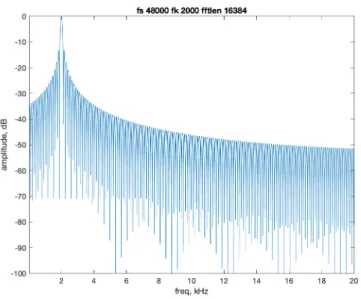
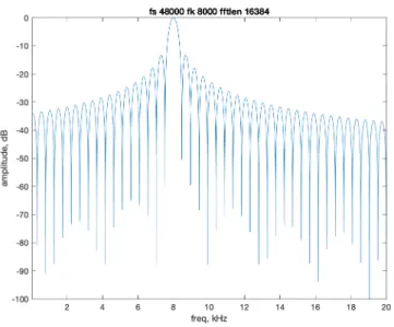
Here, I plot the frequency response of SCFEs for 𝑓𝑘 = 0.5, 1, 2, 4, 8, and 16 kHz. A
constant semitone Q is maintained. See figures (5-2) through (5-7).
Figure 5-2: Constant Q SCFE frequency response for 𝑓𝑘 = 0.5 kHz
Figure 5-4: Constant Q SCFE frequency response for 𝑓𝑘 = 2 kHz
Figure 5-6: Constant Q SCFE frequency response for 𝑓𝑘 = 8 kHz
Figure 5-7: Constant Q SCFE frequency response for 𝑓𝑘 = 16 kHz
A Generalized SCFE
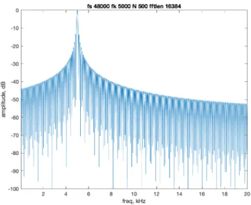
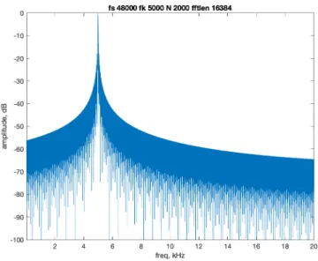
It is possible to increase the frequency selectivity of a general SCFE at any center frequency by adjusting the integration length 𝑁 as desired. This shows the general trade-off between time and frequency, where as 𝑁 is longer, the filter is more frequency selective and as 𝑁 is shorter, the filter is increasingly wider. Here I analyse 𝑓𝑘 = 5
kHz, for 𝑁 = 125, 250, 500, 1000, 2000, and 4000 samples, where the sample rate is 48 kHz. See figures (5-8) through (5-13).
Figure 5-8: SCFE frequency response at 5 kHz, N = 125 samples
Figure 5-10: SCFE frequency response at 5 kHz, N = 500 samples
Figure 5-12: SCFE frequency response at 5 kHz, N = 2000 samples
Figure 5-13: SCFE frequency response at 5 kHz, N = 4000 samples
5.2.2
Alternate Analysis
The following section suggests an alternate z-transform analysis to the SCFE system. I re-frame (5.6) as a traditional discrete time difference equation.
This difference equation has the following z-transform:
𝐻(𝑧, 𝑡) = 𝑒𝑗𝑡Δ𝜃(1 − 𝑒
−𝑗𝑁 Δ𝜃𝑧−𝑁)
(1 − 𝑧−1) (5.8)
I simplify this by letting 𝛼 = 𝑒−𝑗𝑁 Δ𝜃 so the z-transform simplifies to
𝐻(𝑧, 𝑡) = 𝑒𝑗𝑡Δ𝜃(1 − 𝛼𝑧
−𝑁)
(1 − 𝑧−1) (5.9)
The z-transform shows that the system has one pole and 𝑁 zeros with complex coefficients.
5.2.3
Examples
It is possible to analyse just the harmonics of a given musical note by tuning SCFEs to the harmonics of a given fundamental frequency. See figures (5-14) through (5-17). Note that this kind of analysis is equivalent to one column in the M direction of the
Augmented GST.
Figure 5-15: Harmonic analysis of Bb3 on the clarinet
Figure 5-17: Harmonic analysis of G3 on the viola played pizzicato
5.3
Inverse Algorithm
The inverse SCFE algorithm will invert a single channel of analysed audio back into the entire original signal with perfect reconstruction. In Appendix A, it is shown how to modify this algorithms to be used as a monophonic synthesizer. The derivation is straight forward: 𝑓𝑡= 𝑓𝑡−1+ 𝑒𝑗𝜃𝑡𝑥𝑡− 𝑒𝑗𝜑𝑡𝑥𝑡−𝑁 (5.10) 𝑓𝑡= 𝑓𝑡−1+ 𝑒𝑗𝜃𝑡𝑥𝑡− 𝑒𝑗 ⃗𝜑𝑡𝑥𝑡−𝑁 (5.11) 𝑒𝑗𝜃𝑡𝑥 𝑡= 𝑓𝑡− 𝑓𝑡−1+ 𝑒𝑗𝜑𝑡𝑥𝑡−𝑁 (5.12) 𝑒𝑗𝜃𝑡*𝑒𝑗𝜃𝑡𝑥 𝑡= 𝑒𝑗𝜃𝑡 * (𝑓𝑡− 𝑓𝑡−1+ 𝑒𝑗𝜑𝑡𝑥𝑡−𝑁) (5.13)
𝑥𝑡= 𝑒−𝑗𝜃𝑡(𝑓𝑡− 𝑓𝑡−1+ 𝑒𝑗𝜑𝑡𝑥𝑡−𝑁) (5.14)
The algorithm is then as follows: Initialize at t = 1: 𝑓1 = 𝑥1 and 𝜃1 = 0. Δ𝜃 = −2𝜋(𝑓𝑘 𝑓𝑠 ) (5.15) Starting at t = 2: 𝜃𝑡 = 𝜃𝑡−1+ Δ𝜃 (5.16) 𝜑𝑡 = 𝜃𝑡−1− Δ𝜃𝑁 (5.17) 𝑥𝑡= 𝑒−𝑗𝜃𝑡(𝑓𝑡− 𝑓𝑡−1+ 𝑒𝑗𝜑𝑡𝑥𝑡−𝑁) (5.18)
Chapter 6
Geometrically Spaced Transform
6.1
Introduction
The Geometrically Spaced Transform (GST) consists of a bank of Single Channel
Frequency Estimators (SCFEs) whose center frequencies are spaced 𝑓𝑘+1 = 2
1 12𝑓𝑘
apart to model the fundamental frequencies of the notes of the piano. Each channel has a summation constant 𝑁𝑘 that is set to ensure that the channel maintains its
constant Q property. Because 𝑁𝑘 gets shorter with increasing frequency, the GST is
like a wavelet transform; however, there aren’t fewer frequency estimates at higher frequencies than at lower frequecies. Rather, the number of samples used to create the high frequency estimates is fewer than that of lower frequencies. The resulting matrix is rectangular. This is similar to sampling a Continuous Wavelet Transform that is logarithmically-spaced in frequency and linearly-spaced in time. A GST is the first slice of an Augmented GST which is representative of harmonic number one, or the fundamental frequencies of the piano notes.
6.2
Forward Algorithm
Note that for the previous part of the thesis, the algorithms and graphs used a constant N. From here forward, note that N is now set to make the algorithm constant Q and is denoted 𝑁𝑘 for the 𝑘𝑡ℎ frequency channel.
I define x to be the input signal, 𝑓𝑠 to be the sample rate, 𝑁𝑘 to be the window
length of the 𝑘𝑡ℎ frequency channel, B to be the base band frequency, and M to be
the number of frequency channels starting at B Hz.
I compute the center frequencies of each frequency channel based on B and a division of 12 musical notes in an octave:
𝑓𝑘 = 𝐵 * 2
𝑘−1
12 (6.1)
and then the phase update values accordingly:
Δ𝜃𝑘 = −2𝜋(
𝑓𝑘
𝑓𝑠
) (6.2)
For a given frequency channel 𝑓𝑘, I set
𝑄 = 1 2121 − 1 (6.3) 𝑁𝑘 = ⌊ 𝑄𝑓𝑠 𝑓𝑘 ⌉ (6.4) as in [Brown1990]. At t = 1, 𝜃𝑘,1= 0 and 𝑓𝑘,1 = 𝑒𝑗𝜃𝑘𝑥1 = 𝑥1
Consider frequency channel k at time t.
Now for each successive sample starting with t = 2:
𝜃𝑘,𝑡 = 𝜃𝑘,𝑡−1+ Δ𝜃𝑘 (6.5)
𝜑𝑘,𝑡 = 𝜃𝑘,𝑡− Δ𝜃𝑘𝑁𝑘 (6.6)
𝑓𝑘,𝑡 = 𝑓𝑘,𝑡−1+ 𝑒𝑗𝜃𝑘𝑥𝑡− 𝑒𝑗𝜑𝑘𝑥𝑡−𝑁𝑘 (6.7)
summarized as follows, with this time t beginning at t = 0:
𝑓𝑘,𝑡 = 𝑓𝑘,𝑡−1+ 𝑒𝑗𝑡Δ𝜃𝑘𝑥𝑡− 𝑒𝑗(𝑡−𝑁𝑘)Δ𝜃𝑘𝑥𝑡−𝑁𝑘 (6.8)
The algorithm is summarized in the signal flow diagram shown in figure(6-1), which includes a normalization factor of 𝑁1
𝑘. The GST block lengths that make
the algorithm constant Q are shown in figure (6-2). The summation that happens according to the SCFE linear update rule happens over longer windows of samples for lower frequencies and shorter windows for higher frequencies.
Figure 6-2: Block lengths for GST algorithm
The frequency response of the GST is shown for every note A on the piano in figure (6-3) to -60 dB, and for the entire GST filterbank to -12 dB in figure (6-4).
Figure 6-4: Magnitude response of the 88 filters of the GST filterbank
Note that the GST filterbank can be compared to the well known Gammatone filterbank, which is a popular auditory filter model. See figure (6-5).
Figure 6-5: Magnitude responses of 16 gammatone filters in the frequency range 300-8000 Hz
6.3
Calculation of Q
An exact semi-tone Q, according to equation (6.3), would have a value of
𝑄 = 16.817153745 . . . (6.9)
The Q of each frequency channel in the GST can be calculated as follows:
𝑄 = Δ𝜃𝑘𝑁𝑘
−2𝜋 (6.10)
Note that in equation (6.10), because the calculation for 𝑁𝑘 is rounded off, the
Q for the set of 88 frequency channels in the GST is very close to constant, but is not perfect. See figure (6-6). For the GST, the maximum error in the Q for the implemented filterbank is 0.0252. Note the the scale of the y axis in figure (6-6) goes from 16.78 to 16.84, where the desired Q is approximately 16.81. The Q is closer to constant at lower frequencies and the error in the Q is largest at higher frequencies.
6.4
Examples
I present a number of graphical examples of the GST, including an analysis of the piano in figures (6-7) through (6-9), electric guitar in figure (6-10), bass trombone in figure (6-11), and tambourine in figure (6-12).
Figure 6-7: GST analysis of piano note A110
Figure 6-9: GST analysis of piano note A330
Figure 6-11: GST analysis of bass trombone note A110
Figure 6-12: GST analysis of a tambourine slap
6.5
Inverse Algorithm
In Appendix A, it is shown how the inverse GST algorithm can be modified to be a polyphonic synthesizer. The derivation is similar to the inverse SCFE, except that here it is expressed in vector form with K SCFE channels.
𝑥𝑡= 1 𝐾𝑒 𝑗 ⃗𝜃𝑡,𝑘 *𝑇 (⃗𝑓𝑡−𝑓𝑡−1,𝑘⃗ + 𝑒𝑗 ⃗𝜑𝑡,𝑘𝑥𝑡−𝑁𝑘) (6.11)
Chapter 7
Computational Pitch Perception
7.1
Augmented Geometrically Spaced Transform
The Augmented Geometrically Spaced Transform is a matrix of SCFEs that are com-puted for each frequency of the Augmented GST Frequency Matrix (AGST Frequency Matrix). Each entry in the AGST Frequency Matrix contains a center frequency for which an SCFE is computed. Note that for the AGST, non-normalized SCFEs are used. The matrix contains the fundamental frequencies of the piano along the K (fundamental frequency) axis, and then harmonics of these fundamental frequencies along the M (harmonics) axis. See figure (7-1). In comparison, figure (7-2) shows the subset of frequencies in the AGST Frequency Matrix that lie from 20 Hz to 20 kHz. I make the comparison to this figure because in the AGST model, SCFEs are computed for frequencies that lie from 3.4375 Hz to 83720 Hz, which includes frequencies that lie outside the normal range of human hearing which is from 20 Hz to 20 kHz. Note that because the highest computed frequency is 83720 Hz, the sample rate of the system would have to be at least this value to avoid aliasing in the Augmented GST. Typically in audio this would be 96 kHz.
The Augmented GST can be thought of as a movie, where the K x M frequency analysis unfolds over time t. Each snapshot in time is a low level representation of pitch, where the x axis includes the notes of the piano keyboard, but extended by three octaves below the piano in order to be able to represent the pitch from the lowest
Figure 7-1: AGST Frequency Matrix that extends from 3 Hz to 83720 Hz
Figure 7-2: AGST Frequency Matrix that shows which frequencies lie from 20 Hz to 20 kHz
Figure 7-3: Snapshot of AGST of piano note A2
note (A0 with a fundamental frequency of 27.5 Hz) to the highest note (C8 with a fundamental frequency of 4186 Hz). For examples of the AGST taken as a snapshot at time t = 0.1 seconds into a number of piano samples, see figures 3) through (7-6). Note that piano note 37 corresponds to the note A2. Piano note 41 corresponds to C#3. Piano note 44 corresponds to E3. And piano note 47 corresponds to G3.
The system is designed for the purposes of listening to Western music that is tuned to an equal tempered scale based around the note A440, which has a fundamental frequency of 440 Hz. Note here that I use the term augmented because the range of frequencies computed are not just the fundamental frequencies of piano notes but also frequencies that lie both below and above this frequency range. While it is said that the frequency range of listening is from 20 Hz to 20 kHz, I would suggest that the frequencies below 20 Hz and above 20 kHz are not perceived but are still computed by a model such as this one.
7.2
The Summed AGST
In the Summed AGST, spectral energy is summed across the harmonics to produce a single spectral energy estimate that is representative of all of the spectral energy
Figure 7-4: Snapshot of AGST of piano note C#3