y-DYNAMIC ENERGY SYSTEM MODELING -INTERFUEL COMPETITION
by
!Martin L. Baughman
August, 1972
A Report of the
ENERGY ANALYSIS AND PLANNING GROUP School of Engineering
Massachusetts Institute of Technology
Cambridge, assachusetts
)
The Massachusetts Institute of Technology has undertaken a program of research on Energy Analysis and Planning. The overall goals of this program are to develop concepts, information, and an-alytical tools that relate energy supply and demand, the economy and the environment in a manner useful to managers and policy makers in government and the energy industries. The work reported here is the first formal output of this effort.
Further research at refining this model and also developing other models relating to the overall goals of the program is under-way.
David C. White
A B S T R A C T
This work reports the formulation, development, validation, and applications of a medium to long range dynamic model for interfuel
com-petition in the aggregated U. S. The economic cost structure, investment
decisions, and physical constraints are included specifically in the supply models for coal, oil, natural gas, and nuclear fuels, as well as in the consuming sectors residential and commercial, industrial processing, transportation and electricity. The model simulates the development of supply, the fuel selection process in the consuming sectors, the depletion of the resources, and resolves these into fuels consumed cost-price trends in the energy markets of the U. S.
The validation issue is addressed at length through a number of considerations, including comparing the model performance to past
reported behavior of the energy system. It is applied to a series of
scenarios or case studies to assess the impact of a variety of techno-logies, policy considerations, and postulated occurrences on the future energy outlook. Here it is seen the model can be a useful tool, forcing a consistent assessment of possible future trends. The model is useful
for depicting the effects of policy or hypothesized changes in our energy economy in a complete system framework.
This work was submitted to the Department of Electrical Engi-neering at M.I.T. in partial fulfillment of the requirements for the Degree of Doctor of Philosophy (August, 1972).
ACKNOWLED G E M E N T S
ii' iii
I wish to express my sincere appreciation to Prof. David C. White for his guidance and supervision of this work. I also want to thank Prof. Fred Schweppe for his patience, guidance, and encouragement, not only in this work but throughout my whole career at M.I.T.
Many hours of discussion were held with many people in the course of this work for whom much credit is due. However, I would like to es-necially thank Prof. Morris Adelman and Mr. Mike Telson for their in-valuable assistance in the analysis and formulation of the primary fuel supply models contained in this work.
Also, I express my sincere appreciation to my wife Rita, for her assistance in typing the many drafts and understanding support through-out the course of this work.
This work has been supported by the HERTZ Foundation, the National Science Foundation-RANN Division ( Contract # GI-34936) and Massachusetts Institute of Technology Ford Professorial Funds.
The support from these sources is gratefully acknowledged for mak-ing this work possible.
4 TABIE F CONIENTiS Page 2 Abstract . . . . Acknowledgen
Table of Cor
List of Figt
List of Tab] Chapter 1Chapter 2
Chapter 3Chapter 4
Chapter 5 nents . . . . ttents . . . . Ares . . . . es . . . . Introduction . . . .. Model Framework . . . . 2.1 Methodology . . . .. . 2.2 Model Boundaries . . . .. . . 2.3 Levels of Aggregation . . . .2.4 Relationship to Overall Study . . . .
Energy Supply Modeling .. ...
3.1 Primary Fuel Supply . ...
3.? Electricity Supply -- With Nuclear.
3.3 Imports and Exports ...
Dynamics
of Demand
...
...
4.1 Demand Modeling . . . . .. . ...
4.2 Demand Model Behavior .. . .. . .
4.3
Definition
of Demand Model Parameters
4.4 Transportation/istribution
Costs . .
Model Behavior - Model Validation ....
5.1 Model Behavior. . . . . 5.2 Model Validation ... · · · 4·
·... ... 8
9
...
..
15
...
15
... 17...
25
...
28
...
31
. 8 8 * - * 32...
45
...
.57
·
... 58
...
60
...
70
...
73
77 . .. 79 . . * 79... 82
0
5.2.1 Structural Sensitiv 5.2.2 Comparison to Past
5.2.3
Discussion of Base
5.2.4
Further Validation
5.3 Sumnary of Validation Pro
Chapter 6
Chapter 7
Case Studies . . . . 6.1 Case Study No. 1 . . .
6.2 Case Study b. 2. . .
6.3 Case Study No. 3 ..
6.4 Summary
-- Case Studies
Further Research/Conclus ions
7.1 Further Research.
7.2 Conclusions . . . Bibliography . . . . Appendix A Aggregated Model ....
Appendix B Data ...
B. - National Aggregated
B.2 Regional Data . . .
B.3 Data Sources....
Appendix C nvestment and Pricir i
C.1
C.? n Development InvestmeTnvestment in Explor
. · .Data.
nEnerg nt in -at ionC.
Industry Performence. . .
Page
,ity Studies ...
5
Data ...
87
Case Results . . . . .103 Discussions . . . . .107 'ram . . . .109 . . . . .. . . . 111 . . . .111 .. . . . .129 . . . 148 . . . .165 . . . .171 . . . .171 . . . .173 . . . ..175 . . . .177 . . . .184 . . . 184 . . . .194 . . . .20 y upply ... .20 Oil Supply . . . 20? . . . 211 . . . 214 C.4 The Theory as PDlied to the Dynamic Model. . . . .6
Page
Appendix D Model Equations and Base Case Parameters
D. 1 Primary Demand odels . . . .
D.2 Electricity
Demand for Fuels.
D.? Primary Supply Models ....
D.3.1
Natural Gas Supply . .
D. .2 Coal Supply ...
D.3.3 Oil Supply . . . . D.4 Electricity Supply. ... Program Listing . . . .Biographical
Note
....
...
...p227
...
230
... . . . ..236 ... . . . .. 236...
242
* ...
. 2
. . . . 2 44... .255
. . . 273 ... )i0
7
LIST F FIGURES
Pare
Figure 2.1 Overall Model Structure --- Interfuel Competition. . 1Figure 2.2 Table of Assumptions and Important Characteristics . 24
Figure 3.1 Output vs. Time. . . . ... . 33
Figure 3.2 Marginal Development Costs . . . 37
Figure 3.3 Capacity Dynamics --- Primary Fuel Suppliers . . 40
Figure 3.4 Broad Structure --- Primary Fuel Supplier .. . 44
Figure 3.5 Electricity Supply Cost Curves ... . . .47
Figure 3.6 Electricity Supply Dynamics --- Fossil Only. . . . . Figure 3.7 Electricity Supply --- Fossil vs. Nuclear. . . . . 51
Figure 3.8a Fossil vs. Nuclear Cost Calculations ... 53
Figure 7.8b Fossil Fraction Table . ... ... 53
Figure 3.9 Nuclear Fuel . ... 56
Figure 4.2 Dynamic Demand Model ... 69
Figure 4.3 Demand Model Dynamics ... ... 72 Figure 4.4 Distribution Factors vs. Price ... . ... 7L Figures 5.1 - 5.10 Base Case Simulation Results . .. ... 90-99 Figures 6.1 - 6.12 Case Study No. 1 Simulation Results . .116-127 Figures 6.13 - 6.9L Case Study No. 2 Simulation Results . ..135-146 Figures 6.25 - 6.26 Case Study No. 3 Simulation Results. . .152-163
LIST F TABLS Table 4.1
Table
5.1
Table 5.2 Table 6.1 Table 6. Table 6.3 Table 6.4 Table 6.5 Table 6.6 Table 6.7 PageConsuming Sectors --- Fuel Suppliers ... 68
Model Characteristics --- Base Case . ... 89
Base Case --- merical Results . . . 100
Case Study Mo. 1 Characteristics .. . . . .115
Supply Summary Case Study No. 1. ... ..128
Case Study No. 2 Characteristics . . . .134
Supply Summary Case No. 2 ... 147
Case Sturldy N. 3 Characteristics . . . .151
Supply Summary Case No. 3 ... 164
9
CHAPTER 1
INrRODUCT ION10 N
Many economic studies have been done on the supply and price of
each of the various sources of energy [1, 3, 5, 6, 11]. Studies have been made on the determinants of demand for sources of energy 12, 4, 6]. These studies generally refer to the interdependency of price, supply and demand variables that exist among the competing sources of energy, but apparently no one has undertaken to explore in depth the strengths or implications of these interdependencies. This study is an attempt to investigate these mutual cross-ties between the important competing sources of energy in our economy.
In this work, reference to primary sources of energy generally implies coal, oil, natural gas, and nuclear. A secondary source of energy important in interfuel competition is electricity. This is due to its size as a consumer of primary fuels and enhanced by the high degree of substitutability of these fuels in producing electricity. Energy demand refers to uses of fuels for all purposes. These are commonly broken down into the sub-areas industrial processing, space
conditioning (both commercial and residential), transportation, the chemical use of fuel, and electricity (for industrial, commercial, and residential use).
It is true that for many uses in our country the competing sources of energy are highly substitutable. This means that one source of energy can accomplish the user's task as well as another. In 1964, the
10
Energy Study Group wrote
1"While there are some markets for which only one
energy form is now economical,
as much as 95 percent
of total U.S. energy is consumed for purposes in
which several or all of the primary energy sources
are potential
substitutes
(directly
or through
con-version)."
Later works have reinforced this conclusion.
2If one considers the
effects of technological change over sufficient lengths of time, then
100C of energy utilized is substitutable.
The user under these conditions of substitutability
must choose
one fuel over another.
Ris choice may be influenced by price, but
also such things as convenience in handling, cleanliness, and
avail-ability
can enter into his decision making process.
The high degrees
of substitutability characteristic of the sources of energy means that
one cannot discuss the supply, demand,
and
price
of
a
given fuel
with-out also being conscious of the effects of interfuel competition.
This work is an effort to combine the many economic studies of
supply and/or demand for the different forms of energy into a medium
to
long range dynamic model of interfuel
competition for the U.S. This
means that a model containing the dynamic interactions
between supply,
Ener-v
R
+ D and National Progress,
Energy Study Group headed Ali
Bulant Cambel, Lib. Congress Card
Nb.
65-600R7, June 5, 1964, pg. XXV.
2
Gonzalez, Richard J., "Interfuel
Competition for Future Energy Markets,"
11
demand, and price for competing forms of energy is to be constructed. Given the availability of the fuel resources and the levels of demand
for each of the consuming sectors as a function of time, the model will simulate the process by which supply production capacity is
con-structed and resources are depleted, the processes whereby different fuels are chosen to satisfy the demand, and resolve these processes into prices and market shares for each of the forms of supply.
There is no intent in this study to investigate the effects of
seasonal fluctuations of supply and demand on price. For this reason
the effects of storage capacity and processed goods inventories are neglected. Rather, the intent is to concentrate on those phenomena which would have their effect on prices for periods of years, two to
five to ten or more. Those things which have a substantial effect on the dynamics of supply, demand, and prices over the medium to long term as resource depletion, persistent shortages or excesses in
produc-tion capacity, or exploraproduc-tion successes and failures are to be studied.
This is a first application of the dynamic modeling concept to the
interfuel competition processes, which represents a very complex sys-tem. A number of simplifications and approximations were necessary in detail in order to progress on a broad front.
The overall model framework, the model boundaries, the levels of aggregation, and the philosophical approach to modeling this system are discussed in Chapter 2. In Chapter the structure and formulation of
dis-cussed. For ease of presentation, some of the diagrams depicting the model structure in Chapter 3 are in Industrial ynsmics symbology.
In Chapter a description of the demand models end fuel selection pro-cess is given. To the author's knowledge, this is the first applica-tion of demand models in this particular form, and certainly much more work must be done concerning the analysis and plausibility of these models. They are used here because they do represent in an aggregated
way the dynamics of derman and seem to work well in this particular
formulation. Further research is needed to further develop and assess
the implications of this structure.
The validation (or model verification)
issue is addressed at length
in Chapter 5, but in no way represents an exhaustive treatment of the
matter. These validation discussions, along with the application of
the model to a series of case studies in Chapter 6, however do indicate
that the model is credible for a variety of purposes. These same
dis-cussions, nevertheless, point to a number of limitations in the present
formulation and indicate further refinement is needed.
There are three case studies in Chapter 6. The results are
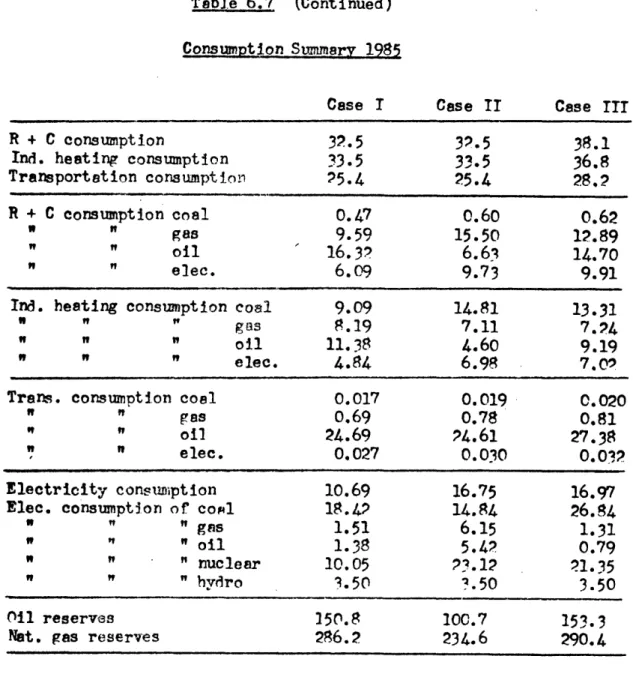
sum-marized in Table 6.7.
In case no. 1, a relatively
optimistic outlook
in oil and natural gs is input to the model, with the result that
cost/price trends for these two fuels remain relatively stable in the
long term outlook. This trend in low prices in oil and natural gas
encourages their use directly
in the residential
and commercial and
1
For a description
of the symbols and their
meaning, the reader may
wish to consult Industrial Dynamics, by Jay . Forrester, published by
13
industrial heating markets, and the growth in electricity
consumption
under these conditions declines to something less than 5% per year,
markedly less than historical trends.
In case
no. 2, a much more restricted
flow of foreign
oil into
this country is hypothesized. This is in contrast to case 1 where by1980 over 50% of the oil supply was supplied by foreign sources. This restricted flow could result for either national security or balance of payments reasons. In addition, environmental constraints are entered into the cost parameters and fuel selection process of the
electricity supply sector in case no. 2. The import quotas and environ-mental constraints combine to yield a much more pessimistic outlook in the future fuel supply trends. For the same domestic supply scenario, prices rise much higher for gas, oil, and electricity.
Finally, in case no. 3, cost escalation in the development of oil and natural gas supplies is entered into the model, and the growth trends in consumption are increased by 25% over the previous case
studies.
The oil import levels
for this case
are
set
the same
as the
National Petroleum Council projection used in case no. 1. Here it can be seen that the increased consumption and escalating costs result in
almost as pessimistic an outlook as that for case no. 2 where much less consumption took place.
By no means are these case studies to be considered proJections by the author. Rather they represent. only an application of the model to
a set of hypothesized conditions to assess the impact of various occurrences an(' usefulness of the model. Within the structural
:3
constraints, the model is found to be useful for a number of applica-tions.
The reader, if not particularly interested in the structural
for-mulation of the model, may wish to only peruse Chapters
, 3, and 4,
and read Chapters 5 and 6 in detail.
In Chapter 7, some areas of
potential further development are identified, and the uses of the
model are summarized.
15
CHAPTER 2 MODEl FRAMEWORK
In the first chapter a general statement of the problem was given --- to develop a dynamic model which characterizes the relationships
important in nterfuel competition. In this chapter a general discus-sion of the methodology and the model framework will be given. The intent is to convey what the major assumptions are on which the model is constructed along with the model bourndaries.
2,1 Methodologl
In order to construct this model, some theory of operation for the interactions between the variables of the model must exist. It is
important to realize that behavior resulting from a model is a con-sequence of the theory on which it is constructed. The model is only
as good as the theory, and the theory is only as good as it helps to explain the real world. For example, one might choose the theory of perfect competition and assume it applies to the behavior of interfuel
competition in the real world. He could build a model, simulate the
interfuel
dynamics, and the resulting
model behavior could be no more
realistic
than the validity
of
the assumptions on which
it
is built.
Unfortunately, in the study of complex systems, assumptions are necessary to keep the study in manageable proportions. Consequently
there usually is not a clear cut answer to the success of the modeling
effort.
The answer is in some respects the model is good, in some
K)
analysis of the ood and bad points is included and they are mnde asexplicit as possible.
However, if it is realized that this work is one step in an
attempt to understand which theories of operations are important and why they are important in the real system operation, then one can under-take the modeling exercise with no reservations about its applicability.
The first question with which one must cope when trying to model a system is "What is the behavior which I wish to explain?" This is the first step in the definition of the system to be modeled. Based on the answer to this question one can then begin to incorporate or discard relationships and variables relevant to the model structure, keeping those that appear to play a role in behavior to be modeled, discarding those that seem to be of no significance. The greater the body of
knowledge about the particular behavior, the easier the modeler's task.
The less that is known about the determinants of the behavior to be
modeled, the more the modeler must make decisions.
In the absence of
a clear cut reasonable choice, the only alternative may be to make an
assumption and later try to verify or violate that assumption. The
final test is whether the model really helps to describe the real
sys-tem which displays the behavior to be modeled within the limitations
of the assumptions made.
For this reason the modus operandi here will be to explicitly
state a theory of operation for interfuel competition under explicit
assumptions, try to assess the applicability of the model through
can-parison of the odel results to past data from the real system, and
17
evaluate what theories require modification to make the model better
conform to the real world process.
The development of a model which
is
a replica
of how the real world behaves is then an iterative
process
of construction, simulation, assessment, modification, construction, simulation, assessment, moification,....etc. With each iteration one gets a better understanding of the important determinants of real world behavior and the shortcomings the model contains. This work describes the results of this process for the dynamics of interfuel competition.
2.2 Model Boundaries
The purpose of this study is to model the mechanisms of behavior important in the dynamics of interfuel competition. Therefore, the model necessarily must contain the interactions between supply and demand within the market clearing process. The market clearing process yields the price and quantity of the different commodities for a given supply-demand configuration; i.e. for the market to clear, supply and demand must be equal. The resulting quantities and prices in turn
affect the rates of growth of both supply capacity and levels of demand. This overall model structure is depicted in figure 2.1.
Figure 2.1 depicts the exogenous inputs to the model as the demand by sectors in the upper portion and the resource characterizations in
the lower portion. The sector demands are assumed to be in time series form for the major corLsuminp sectors (transportation, space
OVERALL MODEL STRUCTURE-INTERFUEL COMPETITION DEMAND BY SECTORS s ENVIRONMENTAL EFFECTS/ REGULAT I N (
I
I I· 2n_
I
I III
I
TECHNOLOG ICAL CHANGE Nb-I
I
I I I I~~~~~1
FUELQUANTITIES/ PRIC E A BOUNDARYMODELI
/-/ EXPLORATION RESOURCE * CHARACTERIZATION 0Figure 2.1
1 0 .) MARKET SENSITIVE DEMAND MARKET CLEARING PROCESS SUPPLY CAPACITY/ COSTS RESOURCESECONOMICAL
TO DEVELOP II _ _ III J,i
_ .r mz
-s---19
growth of demand and also the rates of turnover in the consumers'
equip-merit, some portion of the total demand in the consuming sectors will be
going to the market place to buy energy. This portion of the total
demand is termed the market sensitive
demand in figure 2.1.
The
aggre-gate of those consumers who continue utilizing the same fuels from one
time period to the next is termed the base demand.
Then from considerations on price, the market clearing process
matches up supplies of fuel to meet the market sensitive demand. This
is the classical economic supply-demand equilibrium. In order to model
this
process,
one
needs the supply schedules for each of the
forms
of
supply, demand schedules for each demand sector, and a theory for the market clearing process. From this the quantities and prices for each
of
the
forms
of supply is obtained, which in turn affects the growth in
both the supply and demand sectors.
In general, then, the boundary of the system to be modeled is given by the dashed circle in figure .1. In order for this to be consistent, it is assumed that none of the variables inside the model boundary affect those outside the boundary. The boundary shown in figure ?.1 therefore has some very important implications.
%ne of these is indicated by the dashed line from the box "quantities/prices" to the eogenous input "demand by sectors." In reality it is known that the demand schedule for a commodity is
usually price dependent; that is, as the price goes down the demand
goes
up, and vice versa. The greater the sensitivity of the demand
change to the price changes, the higher the elasticity
of demand.
0o
The measure of elasticity
is
the ratio
of
the percent change demand to
the percent change in price.
Most commodities possess
this
elasticity
because as the price of a given commodity rises, the competing
pro-ducts which will serve the same function become more attractive
price-wise.
Consequently more of the competing products are bought.
If
there is no functional substitute, there may be a choice to do without
the commodity
because of limited resources.
The fact that fuel prices inside the boundary in figure 2.1 does
not affect the exogenously determined "demand by sectors" implies that
sector demands
are assumed
to be inelastic in the model. It is true
that as the price of one form of supply of energy increases, there is
a tendency for the consumers to switch to other cheaper sources of
energy.
This phenomenon is embodied within the boundaries of the model.
The assumption manifested by the dotted line implies that if the price of all sources rose proportionately, the level of total demand would not change. Of course this is not true over the whole range of price
changes possible.
Yet
it
is true that in
our
country
today,
energy
is
and has been a very inexpensive commodity in relation
to its importance.
Expenditures for energy have historically
been about
3
of our gross
national product. Consequently, it may be possible to increase the
price of energy across the board as much as 50 to 100% and it would
have little
effect except in a few highly energy intensive industries.
In other words,
it
is plausible that the demand for energy in toto is
very inelastic in the price ranges that have existed in the past and
those foreseen into the future. Regardless, it will be assumed that
the model such as gross national product, population, nd other demo-graphic variables and can therefore be considered exogenous.
Another implication of the boundaries chosen in figure 2.1 is that
exploration activities and the resulting additions to reserves
there-from are not dependent on variables within the model boundary.
It is
well known that this is not true.
In appendix C there is a discussion
of the exploration incentive.
It is very dependent on the price one
expects to receive for his eventually recovered energy in place. How-ever, the relationship between investment in exploration and the
resulting returns is not well-understood. Certainly more work needs to be done in making these relationships more precise. When this is done, the model is constructed in such a way that the fruits of the research could be included in the structure. Until this is done, it will be assumed that the results of exploration (i.e. additions to reserves and the cost of developing those reserves) are inputs to
model
on the
supply
side
and
independent of those variables
within the
model boundaries.
The basic theory of supply costs and energy prices is derived in
this study
assuming
that the market forces conform to the laws
of
perfect competition. What this means is that over the long term
prices of supply
are
equal to cost (cost including
an
acceptable rate
of return on invested capital).
Over the short term it may be true
that the market forces (in the form of uncertainty about costs
and
deviations from perfect competition) push the price of a fuel above
or below cost. When this happens it only means that the resulting
profits or losses have the effect of either luring new suppliers onto
marketplace or forcing existing suppliers out of the market place until
the law of supply and demand forces price again equal to the long run
costs.
The dynamics of market entry and exit are embodied in this
work.
It might appear that the assumption of perfect competition restricts
the applicability of this modeling effort to the present day energy
sys-tem. However, even though many forms of regulation do exist and
imper-fect competition might exist in the present day energy system, it is
likely that over the long term (decades) the forces of interfuel
compe-tition
from both domestic and foreign energy markets makes the
assump-tion of perfect competiassump-tion realistic.
Further, the theory of perfect
competition is a well-understood economic state of affairs, and thus
provides a convenient starting place for this modeling effort.Never-theless, the model is constructed to be adaptable to pricing strategies
other than the perfectly
competitive
case,
and
this
assumption
is
relaxed after the basic structure is developed.
An area about which nothing has yet been said has to do with the
effect of imports
and
exports on the dynamics of interfuel competition.
In reality the import and export levels of this country are highly
regulated via quotas and duties. In this study the simplification will
be made that imports and exports are exogenous time series input into
the model.
Electricity,
as
a
secondary supplier which utilizes
the primary
fuels and competes on the marketplace with the
primary
fuels, is
not
'
73
diagram. In the work to follow, electricity is dealt with explicitly. At the present time electricity accounts for about 25 percent of our
primary fossil fuel consumption, and this share is expected to grow
until nuclear energy blossoms into a dominant producer in the future.
The leverage that electricity exerts on the primary fuels via the high degree substitutability also warrants the consideration given it in this study. In figure 2.3 think of electricity as simultaneously a supplier and consumer, whose sales to the ultimate consumer are deter-mined in the marketplace, and which simultaneously places a demand on
the primary fuels commensurate
with those sales.
The price of
elec-tricity to the consumer is then related to the price that must be paid
for primary fuels, along with the other fixed and variable costs
per-tinent to that industry. More will be said about this later in thesection on modeling electricity supply.
Figure 2.1 then portrays the mutual interrelationships between the major components of the interfuel system to be explicitly dealt with in this study. This includes the development of supply capacity on the basis of fuel demands and prices and the identification of the market sensitive demand from the dynamics and growth of demand in the various consuming sectors. Then from supply and demand and a theory for the
marketplace, the market is cleared to give fuel quantities sold and the
resulting prices.
These resulting prices then affect the development
of new supply capacity,
(depending on the amount of resources which
Cook, Earl, "The Flow of Energy in an Tndustril
Society," Scientific
TABLE OF ASSUMPTIONS AND IMPORTANT CHARACTERISTICS 1. TOTAL DEMAND INELASTIC.
2. TRANSMISSION/DISTRIBUTION CAPACITY NEGLECTED.
3. TRANSMISSION/,,DIS BiJUTtO- COSTS IN C!UDED AS A
CONSTANT MU' TPLIER OF WH-',' LESALE PRICES.
4. ASSUMED SHORT RUN SUPPLY COST FUi'CTIONALS. 5. DYNAMICS OF MARKET E-TRY INCL UED.
6. EFFECTS OF DEPLETION' OiN CSTS INCLUDED. 7. ELECTRICITY EXPLICIT.
(INPUfS)
RESOURCE SUPPLY CURVES
( NPUTS)
25
are economical to extract at the prevailing prices) and the relative
fuel shares in each of the consuming sectors.
Figure 2.9' summarizes the important assumptions and characteristics
to be followed in the development of the model. Also include i a
broad energy flow diagram to depict the levels of aggregation and
interconnections as they exist in this study.
2.3 Levels of Agregation
It is not clear at the outset what level of aggregation of the
variables or what specific interrelationships
are important to
under-stand these processes. One can only begin at a reasonable starting place and hope to zero in from there. In this first attempt at
modeling the dynamics of interfuel competition there are going to four
levels of supply - coal, oil, natural gas, and electricity.
There are
two reasons for this particular choice. First, this is how much of
the national data is supplied.
Secondly, it is also a logical
extension of previous work. An effort in modeling the complex
inter-actions between the energy, economy, and the environment on a grossly
aggregated level has been done. The work is in its very preliminary
stages, but it does help to motivate this work and orient one into its
realm of applications.
See Appendix A for a discussion and references
to this work.
1For example, the data from the Bureau of Mines and Edison Electric
P6
Due to the levels of aggregation, the price variables in the model
are probably best thought of ss price indices.
They do not apply
specifically to
any
one product (as gsoline, residual oil, stoker
coal, egg coal, or whatever), but to the aggregation of outputs coming
from the same raw fuel source (coel, petroleum, etc.).
There are a
number of ways one might define different indices for this level of
aggregation, as for example an average of product prices weighted by
output mix. In this work the ent.ire sales for all end products
origin-ating frcm the same raw i'uel are lumped together.
Consequently, it is
useful to think of
the
price
variables
in this model as indices of the
ratio of total revenues to total sales in physical units (in barrels,
kilowatt-hours, tons, or whatever).
There are obvious difficulties in lurmping the supply sectors
together on this level of aggregation. Often the growth in supply for
a particular fuel is predicated on the high profitability of a specific
end product, as gasoline from Detroleirj. Since there are technological
limits on the product rnix crirg froi a reflsry, in order to supply
large quantity of gasoline there is created an oversupply of the by-products, or lesser profitable products. This oversupply would drive down the price until enough demand was.5 generated to clear the
market place. The result is tat
the quantity of raw material consumed
is determined by the demand of the highly profitable end product.Consequently, the price of residual oil to
the
electrical
industry
is
in part related to the dremand
for gasoline.
In addition, changing
demand considerat ionrs mqy sh.ift the drive on supply from one output toanother output product.
27
In this work, the problems of primary and by-products are going to
be neglected. This assumes that over the time scales of interest here,
that either the substitutability of users is great enough to keep all
consumption in line with production mixes, or that the production
technology exists to shift the output mix to meet the demand
configura-tion.
In the real world there also exist intermediaries between the
producers
nd consumers of energy. Somehow the energy must be
trans-ported and distributed to the consumer level, and there are costs
involved in this process. In fact for coal the transportation costs
make up about 50, of the selling price. In this model the levels of
transportation capability are not to be explicitly modeled. This assumes that a transportation network exists on a level commensurate with supply and demand. This has not always been true, as the recent oil tanker shortage indicates.
Geographical considerations are not explicitly Included in the
model. This places a number of limitations on the uses of the model
in its present form. For example, the price regulation on the
inter-state sales of naturs gas has resulted in a redistribution
of gas sales
from interstate
to intrastate
markets.
On the
national
level
of
aggre-gation used in the model, this behavior is aggregated away. Many of
the environmental concerns are regional or sub-regional
issues.
These
too are aggregated away in the model. However, the generic
structure
Moyer, eed, Competition in the Midwestern Coal Industry, Harvard
is such that it can be disagpregated for regional or statewide
applica-tiorns. If
this
is done, then the inter-regional links describing the
transportation
capability
muslt be included.
A more complete discussion
of the form the model would take with these cor;siderations included is
given in chapter 7.
The transportation distribution costs are included in a defacto way in the demand models to be discussed in chapter 4. In essence they are assumed to be a constant multiplier of the wholesale prices.
Further discussion of this topic is delayed until the demand models are
discussed in chapter 4.
2.A Relationship to overall stud7
The study and develop.ent of a model for interfuel competition is valuable in itself; but when used in the larger context of the energy systems, it becomes only one gear in a complex machine.
One of the outputs of the interfuel conpetition model is the market shares and levels of consumption for the primary fuels and electricity.
It is well known that the rates of generation of many forms of
pollu-tion in our country are clo3ely related to the utilizapollu-tion of energy
and more specifically to the form of energy used. The model for inter-fuel competition is an important segment of the closed loop process of energy utilization ana pollution eneration, back to envirornental
policy which affects fuel costs and levels of energy utilization.
1See Appendix A.
_I
.v)k
. S
r
29
There are also indications that. low cost energy is a stimulant to economic growth. It is also true that the level of energy consumption is closely correlated to the level of economic output in our country. The interfuel competition model is therefore also an important piece of the closed loop process of economic growth, energy demand, energy costs, and economic growth. In other words, to accurately predict long-term economic growth the role of availability of low cost energy must be included, and the interfuel competition model plays an intricate part in this role. It will be useful to provide data on costs of energy commodities and the level of consumption expenditures for energy given the resource supplies entered into the model.
Similarly, capital investment in energy production facilities is in part influenced by the ease (cost) with which the natural resources can be extracted and processed. The levels of investment activity in
each of the primary fuel suppliers is an integral part of the
dynamic
structure of the interfuel competition model. In addition to affecting
costs of energy in each of the supply sectors, this investment places
a drain on investment funds available to the rest of the economy. There
may be implications for the growth in other sectors of our economy because of this.
The effects of energy costs and utilization upon our environment
ana the potential of economic growth are discussed in "Dynamics of Energy Systems" as problem areas for which is planned in-depth study. The dynamics of interfuel competition is a part of these long term efforts, and the research n this area must keep in perspective the
30
relationship of this study to the overall research proprmn. The fol-lowing chapters discuss in detail the structure and operation of the interfuel competition model. Chapter ? deals with the supply models for both the primary fuels and electricity. Chapter 4 discusses the fuel selection process for the demand sectors modeled. Keep in mind
that the link between the dynamics of supply and the dynamics of demand is the fuel prices.
31
CHAPTER 3
ENERGY SUPPLY MODELING
Introduction
There are basically three subsections of the energy supply models. These are the characterization and dynamics of the marginal development cost curves, the logic and dynamics associated with market entry and sustenance of production capacity, and the cost functional derived from the development and operation of the production capacity. The supply modeling is approached from the level of generality where the equivalent
structure in the primary fuel suppliers is utilizied. Electricity re-quires some modification of this structure to better portray its charac-teristics. Foreign supplies are considered inputs to the model.
This chapter will discuss the models used in energy supply. First will be a discussion of the primary energy suppliers --- coal, oil,
natural gas; nex will be a discussion of the model for the secondary
energy supplier --- electricity (with nuclear); and finally a discussion of the way in whicii foreign sources are entered into the model. In this chapter a general discussion and justification of the models used will be given. In each case it is assumed that the time behavior of each
fuel demand is given. The models then give the dynamic behavior of sup-ply capacity "lnd price. In chapter 4 i is assumed that price is given and the models for the fuel selection process for the demand sectors are developed. Finally in chapter 5 the two pieces are merged and the over-all model behavior is discussed.
32
The content of apperndlx C is drawn upon in modeling the primary
supplies.
Simplifications were necessary due to the limits of
know-ledge.
The major simplification
s that exploration is not modeled,
rather the results of exoloration are inputs to the model.
3.1 Primary Supply MYodel T
Development Cost
?
torm
t
A development cost curve relates the amount of capacity economical
to install on known deposits to the incremental development costs asso-ciated with developir that capacity. A discussion of the formulation of these cost curves follows. For ease of presentation, a discussion
of the formulation for the petroleum industry only is given, but with
changes in terminology it applies equally well to coal.
The development costs for a given reservoir
depend on a number of
things.
These include the size of the reservoir, the capital costs of
capacity construction, and the costs of capital.
Given a reservoir
developed to an initisal capacity qo, the output of that reservoir
(neglecting further development and secondary recovery) would typically
appear as the solid line in figure 3.1.
If a larger initial capacity
aqo
were installed, the depletion of the reservoir would occur faster
as given by the dotted line.
The decrease in output over time
corres-ponds to the effects of depressurization of the reservoir due to
depletion, or for water displacement techniques the shrinkage of the
oil component of the reservoir
due to displacement by water.
The
33 OUTPUT vs. TIME
output
(bbls/da)
. 'I -- , Figure 3.1 q3L
The output of reservoir over time (neglecting secondary recovery) may be approximated by a deciyin exponential. If D is the rate of decline of the output as the reservoir is produced, the output vs.
time, q(t), may be represented by
q(t) = q e Equation 3.1
where q is the initial capacity installed. If RO is the amount of
recoverable resources in the reservoir, assuming that it is fixed
gives
Ro
q
6-Dt
d= q/D
Equation
3.2
or
D = q/Ro
Equation 3.3
That is, the decline rate of output from the initial capacity q is the
ratio of the initial capacity to the total recoverable resources in
place. (Actually this comoutation slightly underestimates D, for wells
do not produce over an infinite lerth of time.),
From appendix C, it is noted that develoimnent is investment in one of two related but distinct options. These include either speedier
recovery of a fixed fraction of the total oil in place, or more
com-plete recovery of the oil in place. Both of these options are an investment in present barrel equivalents (PBE's).
1Bradley, Paul G., The Economics of Crude nOi Production, Nbrth Holland
35
If future output is discounted at a rate "r", the present barrel equivalents from a reservoir with initial capacity q and recoverable oil R is given by
000
PBE =fo q -et qo Equation 3.4
dollarsf, then the b(q mariten rR+ develoment costs (MDC) are given byr
R0
MDunit
cpcity
Equation
3.5
0
The marginal development is the incremental cost of the cost next PBE resulting from investment in more capacity. The marginal development cost function for the reservoir with recoverable oil R and cost per
0
uncost This reatioresship was developed capaer unity b plott. is See AiemA, for one reservoir. The .orld Petroleum For the U.S.97?,Market,2a.
as a rational ngregate, the same analysis applies with a redefinition of terms. For the industry marginal development cost function, the R Thust be defs ins the total U.S. reserves, and "b" as the national average cost per increment in capacity. With this redefinition of terms, figure 3.2s also displays the industry marginal development
cost function.
1
Future operating cts my be discounted nd included in the capital cost per unit capacity. See Aelran, The World Petroleum Market,
John Hopkins Press for Resources for the Future, forthcoming in 1972,
Chapter TI and Appendix.
36
If the industry were operating under the policy of optimal economic choice, then given a price P, the optimum level of supply capacity would be that correspondrin to the value where MDC's were
equal to price as illustrated
in
figure 3.2b. Due to the
uncertain-ties involved other factors infl.nce
the development decision, and
a discussion of how these are mrodeled is given in the next section.
The marginal development cost curve given in figure 3.2b is a
snapshot at one point in time. As reserves get depleted, this
decreases the value of R0 ant moves the curve counterclockwise about
the pivot point "br" (the intersection of the )DC curve with the ordinate axis). Exploration or technological change which increases
the
level
of reserves moves the curve clockwise about the pivot point.
Technological change or new finds which reduce the costs per unit capacity move the entire curve down.
To specify the curve at any instant in time, the only variables
needed are the cost per unit capacity "b", the discount rate "r", and the recoverable resources R0" at that point in time. To specify its dynamics, the effects of exploration, depletion, technological change, and changes in the discount rate must be incorporated. In this work, the additions to reserves (exploration), the cost per unit capacity
(technology), and the discount rate are inputs into the model whose
values are set to correspond to the particular case of interest.
The
depletion is modeled endogenously.
-_1
MARGINAL DEVELOPMENT COSTS
MDC - b(q
+rR
orR 2
Figure 3.2a
INDUSTRY MARGINAL DEVELOPMENT COSTS
* -. .. ., -Re v *. -., !' to Install Figure 3.2b Pric -I I I I I I I I I I v
SupThe ply Ca ty arinamics
The industry marginal development cost curve provies the core of the investment decision process in fuel supply. Given price, the desired intensity of development from economic considerations can be
determined. In reality there are many other factors influencing the
decision processes.
Probably most significant is uncertainty
---uncertainty in costs, ---uncertainty in the general economic
milieu, and
uncertainty in the future.
Also
suppliers
have
goals other than profit
maximization, such as maintenance of market share and growth trends.
There exists regulation which limits one's options, such as prorationing,
price
regulation,
and environmental standards.
All these things as well
as the inAustry structure potentially alter the perfectly competitive decision process. The purpose here is not necessarily to model expli-citly these intervening factors, but rather formulate a model structure
in which, if desired, these influences could be included.
In this work there are essentially two inputs into the investment decision process. These come frorm the marketplace in the form of
1) price and 2) the demand or consumption of that fuel. With these and the assessment of the factors influencing costs the development decision
is modeled.
The factors determining the marginal development cost function were
given in the last section. Suppose for the moment that a reasonable
value for price, or more precisely the projected price, is available to
the investors in supply. Actually the price used here is derived from
the smoothed short run market fluctuations of price in the marketplace,
;
and how it is formulated in the model will be discussed shortly.
Given
this price the desired capacity from economic considerations is deter-mined as in figure 3.?b. From trends in consumption or sales, the capacity required to serve expected future levels of demand can also be calculated. The capacity development logic of the programmed model then uses these projections on price and consumption and includes an assessment of the productivity of present capacity in simulating the rate of capacity development.
However, this capacity does not become productive immediately. It takes time to allocate the resources (planning, men, machinery) to a particular development, and once construction begins a time delay : exists before the development becomes productive. To model these
processes, a first order exponential delay followed by a third exponen-tial order construction delay is used. The first order delay models
the perception and allocation delays associated with the initiation of
construction. The third order delay represents the construction delay
from the initiation to completion of development. This process is
shown symbolically
in the flow
chart
in figure
3.3.
The
period
of time over which the projections
are made corresponds
to the construction delay, or the length of time it takes to get new capacity operable. Also represented in figure 3.3 is the decline in productivity corresponding to the depletion rate. This is to model the exponential decay in output as shown in figure .].
With these basic components the supply capacity dynamics are modeled. To be discussed yet is the relationship between these long
run supply dynamics and the short run cost-price
dynamics in the
marketp] ace.
o40
CAPACITY DYNAMICS - PRIMARY FUEL SUPPLIERS
DEMAND _ PREDICTED
t |
0~~~~~~DE
ok
MA
ND
I
. / I I I RESERVE 116. %%1 / I I I MARGINAL DEVELOPMENT COST FUNCTION (MDC)-
r
T
COST OF / CAPITAL I " I I4-COST PER UNIT CAPACITY I ENTRY TIME CONSTANT
\
I I I III I I I I I IDI
DESIRED UTILIZATION Figure 3.30
-. !l41
Modeling this short term behavior would be unnecessary in this work if only the long run supply-cost relationships were important.
However, it can be true that a short run disturbance can sufficiently alter the supply picture that it may take years for the system to recover. In particular the effects of the relatively recent environ-mental concerns, which have become national issues in Just a few years,
are perturbing the supply-demand relationships enough to result in severe shortages of environmentally desirable fuels.
The long run price trend for a particular fuel is the collection
of the random short run price fluctuations in the marketplace. In a
certain
world, it would be easy and
logical
to price
output
at marginal
development cost defined previously. In truth the world is not certain:and the industry marginal development costs at any point in time are
not easily ascertained.
Some random behavior in the dynamics of demand
exists,
expected development times and acquisition delays may not
materialize due to environmental concerns, capital and labor costs may
change. All these things affect the supply-demand relationship so that
in truth the system may never reach the equilibrium price, but rather
it only equilibrates about the equilibrium.
As these disturbances change the supply demand configuration, the
price changes over the short term in reaction. The short run supply(capacity fixed) is less elastic than the long run so that small changes
in the supply-demand configuration can cause relatively
large
fluctua-tions in the short run costs of supply. It is these smoothed short run
fluctuations that indicate to the supplier how his particular fuel is
47
faring on market place vis-a-vis the competitive fuels.
The short run costs are meae up of the operating
and
maintenance
expenses of sustaining
output from that capacity.
In this work an
assumed functional relatiornship is used for the short run cost curve.
This relationship is constructed in the perfectly competitive case so that if the utilization of existing supply is at the desired level, the short run marginal cost equals the marginal development costs. If the capacity is being under utilized, the short run marginal cost is
less than the marginal developler.t cost, a if existing capacity is being utilized over the esired (optimum) utilization level the short run marginal cost is reater than the marginal development cost. In other words the long run equilibrium price is assumed to be the value of the marginal development cost. On the short term, price may
fluc-tuate above or below this equilibrium value. If price goes above the marginal development cost, this encourages further development until costs are again equs' to price. Tf price goes below the marginal development costs fur-ther development is discouraged.
This assumed short run marginal cost function can be written as
follows:
SRMC = (MDC) a Equation 3.5
where SR1 is the short run marginal cost M)C is the marginal development cost
is the level of production capacity
C~~~~Q
is the level of fuel demand
a is the planned surplus capacity.
If the actual utilization is equal to the desired utilization, the SRMC of equation 3.5 is equal to the MDC. If the actual utilization is different than the desired, the short run costs are assumed to behave in accordance with equation 3.5.
The price of a particular fuel does not track exactly the short run marginal costs. In reality these are probably not known at any point in time. Rather these costs are smoothed as data on daily or weekly or monthly operations is gathered and analyzed. A firm then uses.this data (along with all the other factors pertinent to its pricing policy) to determine price. So in essence the price of a par-ticular fuel on the marketplace is a function of the smoothed value of the industry aggregate short run marginal costs. Tt is this price
on whic- consumers make their fuel selection decisions and it is this
price nd its trends which suppliers use in their investment decisions. This short run cost-pricing structure is superimposed on the model structure of figure 3.3 and given in figure .4. This then completes the generic structure for primary fuel supplies coal, oil and natural gas. The primary inputs to the model are the aditions to reserves and the cost per unit capacity. The fuel demand is derived from the demand side of the interfuel competition model discussed in chapter 4. Parameters such as time constants, delays, prediction intervals, etc. -must be set to conform to the particular form of supply of interest..
BROAD STRU(:'TUR
PRIMARY FUEL. SUI'PPI.I.R
(OAl, O11.. NAIURAI. (A' I '[)I~?Ar
(MDC) ,
-/ \
-4---COST OF COST PER UNIT
CAPITAL CAPACITY Figure 3.4 I I I I \\ I I I / AT ION
L5
3.? Electricity Supply -- with Nuclear
Electricity, as an energy supplier, is unique in that it has no energy storage capability. Because of this, the capacity levels re-quired to maintain a reliable supply are governed by the peak power requirements and not the average output levels. Due to this and the capital intensiveness of the industry, it means that in figure 3.5 the
industry can be operating to the left of the minimum
on the AC curve,
or MC's are less than AC. Further, there exists the option of using
nuclear energy in electricity supply, the only place where it is com-petitive on a large scale in the energy system. Consequently, to more accurately model electricity supply it is necessary to deviate from the primary fuel supply models given in section 3.1.
This deviation is substantial in three aspects. First the role of the nuclear generation option must be defined and included in the model. For ease of presentation, however, let's postpone a discussion of
nuclear in electricity supply and assume only fossil fueled generation exists. Once the structure of electricity supply with fossil only is
discussed then the role of nuclear will be included.
A second deviation of the electricity supply model from the primaxy
supplier models is that electrical output is priced at average cost
rather then the long run marginal cost level. This is in reality what the regulation in electricity rate structures attempts to achieve.Finally, the decision to build new capacity is the result of trade-offs in economics and reliability. To supply electricity at lowest cost, it is desirable to keep reserve capacity (excess capacity over
46
and above peak output requirements) as smll as possible so that t given level of electricity demand (QD in figure ?.5) the AC curve is nearer the minimum. Counter to this, to reliably meet peak power
requirements, there is a desire to keep excess reserve capacity
---which moves price up the left
portion
of the C
curve.
The optimum value of reserve capacity is the minimum
needed to
reliably meet peak
power
requirements. The cost of the energy delivered
is related to the peak to average
output,
or
the
capacity
utilization
factor.
The capacity utilization
factor (CUF) is defined here as
Energv Delivered in kh.Z
)
Capacity Installed
(in kw. j x hrs./year
=
CUF
This is nominally in the neighborhood of 0.5 to 0.6 for the U.S.1
Such things as pumped storage or the overnight battery charging of the
electric cars have the potential of increasing this number substantially,
and thus reducing average costs.
The decision to build new production capacity is then based simply
on projections of peak power requirements. An overcapacity penalizes the
supplier with higher than necessary average costs.
An undercapacity
results in a deficiency in reliability and quality in service to cus-tomers (brownouts; etc.). In the model the capacity requirements are
based on projections
in electric
energy consumption divided by the CUF.
The projections
in consumption are made vie a simple quadratic least
squares curve fit to the previous 20 years consumption. These
projec-tions are made over a length of time corresponding to the siting
and
Calculated from
FFT
St.atist.ical Yearbook, various issues from annualdata on capacity end delivered energy.
4'
ELECTIRCITY SUPPLY COST CURVES
Costs Al I I I
Q-
,Q-
Q
Figure 3.5 Price i Lconstruction delay in building a new plant. The CTIF is parameter that must be set to correspond to the particular characteristics of the electrical load being investigated.
The model for electricity supply with fossil only is depicted in figure 3.6. In addition to those things already mentioned, a couple of other details need discussion.
The costs of electricity supply are made up of basically two com-ponents. These are the capital costs of plant construction and the
variable costs of plant operation. These variable costs are made up
of the operating and maintenance costs and the fuel costs incurred in
normal plant operation.
In this work it is assured that a constant
fraction of the plant investment is written off each year and allocated
to the output. This fraction is called the annual capital charge rate.
The average fixed costs associated with a unit output in any given year
is then the capital write-off for that year divided by the output for that year. The average vriable costs are the average operation and maintenance costs and the average fuel cost per unit output. The
average fuel price is assumed to be the weighted average of the prices of the competing fossil fuels, weighted by the fraction of electrical output supplied by each fuel. The details of the selection process for fuels in electricity supply are discussed in chapter . The amount of primary fuel required to produce a given level of output is determined by the heat rate which also affects the average fuel costs. These
ELECTRICITY SUPPLY DYNAMICS FOSSIL ONLY REGRESSIVE CURVE FIT / PREDICTED DEMAND / / __ Figure 3.6 EL DEr