Wigner matrix formalism for phase-modulated signals

HAL Id: hal-03215977

https://hal.archives-ouvertes.fr/hal-03215977

Submitted on 3 May 2021

HAL is a multi-disciplinary open access

archive for the deposit and dissemination of

sci-entific research documents, whether they are

pub-lished or not. The documents may come from

teaching and research institutions in France or

abroad, or from public or private research centers.

L’archive ouverte pluridisciplinaire HAL, est

destinée au dépôt et à la diffusion de documents

scientifiques de niveau recherche, publiés ou non,

émanant des établissements d’enseignement et de

recherche français ou étrangers, des laboratoires

publics ou privés.

Wigner matrix formalism for phase-modulated signals

H. Coïc, C. Rouyer, Nicolas Bonod

To cite this version:

H. Coïc, C. Rouyer, Nicolas Bonod. Wigner matrix formalism for phase-modulated signals. Journal

of the Optical Society of America. A Optics, Image Science, and Vision, Optical Society of America,

2021, 38 (1), pp.124-139. �10.1364/JOSAA.408363�. �hal-03215977�

Wigner Matrix Formalism for phase modulated signals

H.

C

OÏC

,

1,*

C.

R

OUYER

,

1

AND

N.

B

ONOD

2

1 _{CEA-CESTA, F-33116 Le Barp, France} 2 _{Aix-Marseille Univ, CNRS, Centrale Marseille, Institut Fresnel, Marseille, France} *Corresponding author: herve.coic@cea.fr Received XX Month XXXX; revised XX Month, XXXX; accepted XX Month XXXX; posted XX Month XXXX (Doc. ID XXXXX); published XX Month XXXX Laser beam can carry multi-scales properties in space and time that impact the beam quality. The study of their evolution along complex optical sequences is of crucial interest, particularly in high intensity laser chains. For such analysis, results obtained with standard numerical calculus are strongly dependent of the sampling. In this paper, we develop an analytic model for a sinusoidal phase modulation inside a sequence of first order optics elements based on the Wigner matrix formalism. A Bessel decomposition of the Wigner function gives pseudo-Wigner functions that obey to the general ABCD matrix law transformation without approximations and sampling considerations. Applied to a Gaussian beam, explicit expressions are obtained for the projections of the Wigner function in the sub-spaces and gives a powerful tool for laser beam analysis. The formalism is established in the spatial and temporal domain and can be used to evaluate the impact of the phase noise to the beam properties and is not limited to small modulation depths. In a sake of illustration, the model is applied to the Talbot effect with the analysis of the propagation in the spatial and phase-space domain. A comparison with full numerical calculations evidences the high accuracy of the analytic model that retrieves all the features of the diffracted beam. http://dx.doi.org/10.1364/AO.99.099999

1. INTRODUCTION

Wigner Distribution Function (WDF) [1] has been successfully used to study the propagation of optical beams through first-order optical systems [2]. WDF is a signal representation in space (time) and frequency simultaneously and this forms an intermediate signal description between pure space (time) representation (electric field) and pure frequency representation (spectrum).

ABCD matrix formalism is widely used technique to evaluate the output beam properties of laser chains including beam propagation, imaging and focusing with lenses for high energy lasers [3,4], and also stretching and compression with gratings for high power lasers [5]. Accurate numerical modelling of such laser chains containing multi-scale considerations in space and time requires important computing resources and is subject to numerical imprecisions. In this paper we propose a general model obtained by coupling the Wigner approach [2] with the ABCD matrix formalism without approximations and errors induced by numerical sampling. Moreover, it allows to extract significant physical parameters from a specific laser chain. We show how the association of these two powerful techniques allows to model the impact of a coherent and incoherent phase noise on the optical properties of the beam. The general model is valid in the spatio-temporal domain and the phase noise can be added to a perfect beam and inserted in any ABCD matrix sequence. This allows to model imperfections of any optical components inside the laser chain and to evaluate its impact in the output beam quality.

The coherent phase noise modeling is based on the Bessel decomposition of the sinusoidal phase modulation [6,7], by analogy

with the decomposition of the cross-spectral density function for Bragg diffraction [8]. This decomposition gives pseudo-Wigner functions that obey to the general Wigner ABCD matrix transformation. Studying the evolution of the elementary pseudo-Wigner function through ABCD transformation provide a complete description of the beam by coherent addition of the pseudo-Wigner function obtained after the ABCD transformation. The analytical approach allows to model the impact of high frequency phase modulation in the propagation of large laser beam. Let us notice that the Bessel decomposition is not limited to small modulation of the phase noise. The formalism presented in this work can be also used to model strongly modulated signals in both spatial and time domains. Strongly modulated signals turn out to be of the highest importance in high energy laser chains. The phase of signal can be modulated in the time domain for avoiding Brillouin and Raman scattering [9] and for beam smoothing [10,11] in high energy laser chains. The contents of the paper are as follows. In section 2 we analyze the decomposition of the Wigner function of a spatially phase modulated signal with sinusoidal modulation at the frequency Kd/2π, and can be viewed as a coherent analysis of interacting beams. We show that the Wigner function can be written as the sum of pseudo-Wigner functions using the Bessel decomposition of the phase modulation function. These pseudo-Wigner functions obey to the standard linear ABCD matrix transformation. In section 3, we establish a matrix formalism for a phase modulated signal in the general case where the phase mask which creates the phase modulation is positioned anywhere in a sequence of linear optical components. In section 4, for comparison, we develop an equivalent matrix formalism for the Gaussian-Schell Model (GSM), which is the Wigner model for incoherent or partially coherent

beams. For the incoherent phase noise treatment, Gaussian-Schell model (GSM) has been intensively used to model partially coherent beams [12,13] and is well adapted to model imperfections of optical components. A matrix formulation is proposed to transform in a sequence a coherent beam to an incoherent beam. In section 5, we apply the model to Gaussian beams. In this case, the Wigner functions and their projections in the different sub-spaces are described with analytical expressions featuring a Gaussian formulation, avoiding imprecisions induced by numerical integration. In this part, the Wigner projection in the spatio-temporal domain is described, and gives the exact formulation of intensity I(x,t), fluence F(x) and Power P(t) of the pulse. In section 6, we apply the Wigner Bessel decomposition to the analysis of the Talbot effect. The Bessel decomposition in power series for five contributions, respecting the energy conservation, allows an explicit formulation for the Talbot effect in the spatial domain for finite size beams. The first application is the analysis of the Talbot effect in the phase space domain (x,kx) with dimensionless parameters which allows to observe invariant quantities. A comparison with the GSM beam is proposed and can be easily extended to the 2D phase space domain (x,y,kx,ky). A second illustration is the analysis of the Talbot effect in the spatial domain, which corresponds to a transformation of a phase modulation to an amplitude modulation with the propagation. Such properties cannot be obtained with GSM model which only treats the evolution of average quantities while the Bessel decomposition gives interferometric information.

2. WIGNER FORMALISM FOR PHASE MODULATED

SIGNALS

A. Wigner formalism

Let us consider, in the spatio-temporal domain, an electric field E(x,t). The corresponding Wigner function can be written as [2] with the convention of positive argument for Fourier transformation:

( )

[

]

* 0 2 1 1 1 1 1 1 1 1 1 1 1 1 1 ( , , , ) , , 2 2 2 2 2 exp x x W x t k E x x t t E x x t t ix k it dx dt ω π ω ∞ ∞ −∞ −∞ ⎛ ⎞ ⎛ ⎞ = _⎜ + + _{⎟ ⎜} − − _⎟ ⎝ ⎠ ⎝ ⎠ × +

∫ ∫

(1) For linear transformations, the ABCD matrix law gives [14]:

(

) (

)

(

) (

)

(

)

0 ( , , , ) , , , , , , , , , , , , , , , Seq x x x x x x W x t k W X x t k T x t k K x t k x t k ω ω ω ω ω = Ω (2) where the functions X, T, Kx, and Ω express the transformation of the arguments of the Wigner function with ABCD matrix. This allows considering only the arguments transformation instead of the function transformation.

For Gaussian beams, the Wigner function and its projections into the different subspaces are Gaussian (see Part 5). For a standard initial Gaussian beam of spatial and temporal size Δx and Δt, and a total energy Et: 2 2 0 2 2 2 ( , ) exp π ⎡ ⎤ = _⎢− − _⎥ Δ Δ ⎣ Δ Δ ⎦ t E x t E x t x t x t (3) The Wigner function is [15]: 2 2 2 2 2 2 0 2 2 2 2 2 ( , , , ) exp 2 2 ω ω π ⎡ Δ Δ ⎤ = _⎢− − − − _⎥ Δ Δ ⎣ ⎦ t x x E x t W x t k x t k x t (4)

B. Sinusoidally phase modulated electric field and Bessel decomposition Let us consider now, in the spatio-temporal domain, an electric field E0(x,t) interacting with a spatial sinusoidal phase mask with of period 2π/Kd and modulation depth m. The resulting field can be expressed as a sum of an infinite Bessel decomposition:

(

)

[

]

0 0 ( , ) ( , )exp sin ( , )=+∞ ( )exp =−∞ = ⎡_⎣ ⎤_⎦ =

_∑

d n n d n E x t E x t im K x E x t J m inK x (5) where Jn represents the Bessel function of the first kind of order n. The zero order contribution (n=0) is proportional to the field component transmitted without perturbations. We can reduce the analysis to the field Kernel Gn(x,t):

[

]

0 ( , )= ( , )exp n d G x t E x t inK x (6) to describe the electric field: ( , ) =+∞ ( ) ( , ) =−∞ =

_∑

n n n n E x t J m G x t (7) For the field Kernel Gn(x,t), the equivalent of the Wigner function is:

( )

[

]

* , 2 1 1 1 1 1 1 1 1 1 1 1 1 1 ( , , , ) , , 2 2 2 2 2 exp n l x n l x W x t k G x x t t G x x t t ix k it dx dt ω π ω ∞ ∞ −∞ −∞ ⎛ ⎞ ⎛ ⎞ = _⎜ + + _{⎟ ⎜} − − _⎟ ⎝ ⎠ ⎝ ⎠ × +

∫ ∫

(8)

This function is not rigorously a Wigner function because it corresponds to a conjugation of the electric field Kernels with different orders n and l, and it is a complex function. Let us describe two properties of this function: * ,( , , , )

ω

= ,( , , , )

ω

n l x l n x W x t k W x t k (9) and: , ( , , , )ω ( ) ( ) ( , , , )ω =+∞ =+∞ =−∞ =−∞ =

_{∑ ∑}

n l x n l n l x n l W x t k J m J m W x t k . (10) The fact that * ,( , , , )

ω

= ,( , , , )

ω

n l x l n x W x t k W x t k allows us to prove that W is real: , ( , , , )ω ( ) ( )Re( ( , , , ))ω =+∞ =+∞ =−∞ =−∞ =

_{∑ ∑}

n l x n l n l x n l W x t k J m J m W x t k (11) In the following parts, we will reduce our analysis to the pseudo-Wigner function Wn,l(x,t,kx,ω), which include self-Wigner terms (n=l), and cross-Wigner terms (n≠l,) [16].

C. Wigner function for Gaussian beam

The Wigner formulation with ABCD matrix formalism applied to Gaussian beams gives specific relations between the electric field and the Wigner function [17,18]. For a phase-modulated signal applied to a Gaussian beam, the pseudo-Wigner function is:

(

)

, 2 2 2 2 2 2 2 2 2 ( , , , ) 2 2 exp _{2 2 2} exp ω π ω = ⎡ _{Δ ⎛ ⎛ + ⎞ ⎞ Δ} ⎤ × ⎢−_Δ −_Δ − ⎜ +⎜ ⎟ ⎟ − ⎥ ⎝ ⎠ ⎝ ⎠ ⎢ ⎥ ⎣ ⎦ × ⎡_⎣ − ⎤_⎦ t n l x x d d E W x t k x n l t x t k K x t i n l K x (12) The spatial phase modulation induces a shift in the kx space for the amplitude. This expression can be then reduced to:

(

)

,( , , , )ω 0 , , ₂ ,ω exp ⎛ ⎛ + ⎞ ⎞ = _⎜ +_{⎜ ⎟ ⎟} ⎡_⎣ − ⎤_⎦ ⎝ ⎠ ⎝ ⎠ n l x x d d n l W x t k W x t k K i n l K x (13) or, in an equivalent representation:

(

)

, 0 2 ( , , , ) ( , , , ) exp _{2 2} 2 ₂ exp ω = ω ⎡ Δ ⎛ + ⎞ ⎛ ⎛ + ⎞ ⎞⎤ × _⎢− _{⎜ ⎟ ⎜} +_{⎜ ⎟ ⎟⎥} ⎡_⎣ − ⎤_⎦ ⎝ ⎠ ⎝ ⎝ ⎠ ⎠ ⎣ ⎦ n l x x d x d d W x t k W x t k x n l _{K k} n l _{K i n l K x} (14) It shows that the pseudo-Wigner can be written as: ● the product of the Wigner function of the initial field containing modulated term with an exponential function containing linear phase term in x. ● or the product between the Wigner function of the initial field, not modulated, with an exponential function of linear amplitude term in kx and a linear phase term in x. In the following part, we study the evolution of the Wigner function with the matrix formalism and show that we can always write the Wigner function in those two representations.

3. MATRIX FORMALISM

In this section, we aim at describing separately the different elementary transformations of the pseudo-Wigner functions needed for describing a complete ABCD sequence transformations and phase modulation. In the proposed model, the phase modulation can be positioned anywhere on the sequence, it is the reason why we consider an ABCD transformation M0 followed by a phase modulation, and

followed by a second ABCD transformation M1. A. Matrix formalism for a phase modulated signal The arguments of the initial Wigner function are denoted into the form of a column matrix: ω ⎛ ⎞ ⎜ ⎟ =⎜ ⎟ ⎜ ⎟ ⎜ ⎟ ⎝ ⎠ x x t k r , (15) The Wigner expression of the field is then given by [2]:

( )

(

)

0( ) ₂ exp det

π

= Et − W T -1 r r Qr Q , (16) where T denotes the transpose of the matrix column r and where the matrix Q represents the Curvature Matrix [19], which is also equivalent to the inverse of the 2nd _{order matrix moment of the field [20]. Q is real} symmetric, positive definite and symplectic [17]. Integration over the four arguments (x,t,kx,ω) gives the total energy Et of the beam: 0( ) =

_∫

t E W r rd , (17) with det

_{( )}

Q-1 =1.

If the phase of the initial field is modulated, the pseudo-Wigner functions are given by:

(

) (

)

(

)

(

( )

)

,( ) 2exp exp t n l E W i

π

= − n,l T n,l n,l T r r + S Q r + S D r , (18) with:

(

)

(

)

3 1 2 d d n l K n l K + = = − n,l n,l S I D I , (19) and, 3 0 0 1 0 ⎛ ⎞ ⎜ ⎟ =⎜ ⎟ ⎜ ⎟ ⎜ ⎟ ⎝ ⎠ I , 1 1 0 0 0 ⎛ ⎞ ⎜ ⎟ =⎜ ⎟ ⎜ ⎟ ⎜ ⎟ ⎝ ⎠ I . (20) It can be noticed that the phase modulation induces an additional linear phase term and a modification of the amplitude of the pseudo Wigner function. The matrix formalism is very convenient since it allows to address also phase modulation in the time domain or even both spatial and time domains considering the right choice of Sn,l_{, D}n,l_, and I column matrices. Wnl are self (n=l) or cross (n≠l) Wigner terms. The self-Wigner terms are real (Dnl=0) and they transport the energy of the beam on the even (n+l=2n) contributions. The cross-Wigner terms have a non-null phase complement (Dnl≠0). They don’t carry energy if the number of fringes is significant in the field envelope (i.e. cos[(n-l)Kdx]≈0 in mean value). The (n+l) contribution of the pseudo-Wigner terms can be even or odd, but the odd contributions are composed with only cross-terms without energy. It will be illustrated in Part 6 in Fig. 1 and Fig. 2. B. ABCD transformation of an initially phase modulated field Let us now consider the impact of an ABCD transformation M1 on the

pseudo-Wigner function. If M1 represents the 4x4 ABCD matrix

describing the transformation of the argument r through a first order optical system, then, the evolution of the pseudo-Wigner function after the transformation is given by:

(

) (

)

(

)

(

( )

)

1 , , 2 ( ) ( ) exp exp M n l n l t W W E i π = = − 1 T T n,l n,l n,l 1 1 1 r M r M r + S Q M r + S D M r . (21) This transformation corresponds to the change: 1 → r M r . (22) The ABCD transformation law is applied only to the column matrix r and not to the Sn,l _{because ABCD law acts only on quadratic terms for}

Gaussian beams. For first order optical systems, ABCD matrix are symplectic [7,14].

C. ABCD transformation for a field without modulation to the phase mask component

We now consider the case of the ABCD transformation M0 before the

phase modulation, i.e. for a beam without phase modulation. In this case the transformation through ABCD matrix M0 is:

(

)

(

)

(

)

0 0 ( ) 0( ) 2exp . M Et W W π = 0 = − 0 T 0 r M r M r Q M r (23) If, after this ABCD transformation, the field is modulated in phase, the pseudo Wigner function becomes:

(

)

(

)

(

(

)

)

(

)

( )

(

)

0 ( ) , ( ) 2exp exp . M x t n l E W i ϕ π + = − × T n,l n,l 0 0 T n,l r M r + S Q M r + S D r (24)

An important remark has to be done at this stage: if the field is transformed with an ABCD sequence followed by a phase modulation, the M0 matrix transformation acts both on r and Sn,l components.

D. Phase mask in a middle of an ABCD sequence

We now consider the complete sequence of a phase mask located between two 4x4 M0 and M1 matrices. By combining the results

derived in the last two sections, we obtain the following pseudo-Wigner function of the complete sequence:

(

)

(

)

(

(

)

)

(

)

( )

(

)

, 2 1 1 1 ( ) exp exp , Seq t n l E W i π = − × T n,l n,l 0 0 T n,l r M M r + S Q M M r + S D M r (25) which is also equivalent to:

(

) (

)

(

)

( )

(

)

, 2 1 1 1 ( ) exp exp . Seq t n l E W i π = − × T n,l n,l 0 0 0 0 T n,l r M M r + M S Q M M r + M S D M r (26)

This general expression can be used for any linear ABCD transformation, including propagation and focusing in the spatial domain, dispersion in the temporal domain, but also the spatio-temporal coupling via diffraction gratings stretching and compression of the beam. An alternative formulation can also be found by writing:

(

)

, ( )= 0 ( )exp ,( )+ Φ,( ) Seq Seq n l n l n l W r W r A r i r , (27) with:

(

)

(

)

(

)

(

)

(

) (

)

(

)

(

)

(

)

( )

( )

0 0 1 2 1 1 , 3 1 1 3 2 2 3 3 , 1 ( ) ( ) exp ( ) 2 2 ( ) ( ) Seq t n l d d n l d E W W n l A K n l _K n l K π = = − + ⎛ ⎞ = −⎜ ⎟ ⎝ ⎠ ⎡ ⎤ × + ⎣ ⎦ + ⎛ ⎞ −⎜ ⎟ ⎝ ⎠ Φ = = − T 0 0 0 T T 0 0 0 0 T 0 0 T T n,l 1 1 r M M r M M r Q M M r r M I Q M M r M M r Q M I M I Q M I r D M r I M r (28) It shows that the complete Wigner function can be written as the product of the Wigner function without phase modulation with a sum of amplitude and phase terms, as the formulation established in section 2.C:

(

)

0 , , ( ) ( )=+∞ =+∞ ( ) ( )exp ( ) ( ) =−∞ =−∞ =

_{∑ ∑}

+ Φ n l Seq Seq n l n l n l n l W r W r J m J m A r i r . (29) E. Discussion

The formulations (26) or (27) can be used for modelling and visualizing the impact of the phase modulation on the middle of complex optical sequences and are directly applicable to high laser chains [3-5] containing not only propagation, but lenses, gratings etc... Compared to classical numerical calculation (FFT based algorithms), (26) or (27) takes the advantage to carry multiscale properties (1/Kd<<Δx for example) without approximations and errors induced by numerical sampling.

The Bessel decomposition presented here can be extended to any periodic signal by replacing Bessel Jn and Jl coefficients by the general Fourier series decomposition (plane waves decomposition). In the same way, the amplitude envelope of the electric field E0(x,t) can be decomposed in sum of off-axis Gaussian fields (see for example [21] for supergaussian decomposition). Decomposition of periodic signals and amplitude envelope on Gaussian basis are very similar on the Wigner domain: ● an amplitude shift in kx (respectively ω in the time domain) for periodic signals, or in x (respectively t) for the envelope decomposition. ● a phase shift in x (respectively t) for periodic signals, or in kx (respectively ω) for the envelope decomposition.

In the other hand, a matrix representation of the Wigner formalism allows to represent the evolution of the second order moments of an arbitrary beam. Let us point out that the study of arbitrary beams limited to their second order moments reduces to a Gaussian representation.

To obtain the physical observables (intensity, fluence, power etc..), it is necessary to project the Wigner function in the sub-spaces. At this step, it is obtained by numerical integration of formulations (26) or (27). In Part 5, we propose a new step consisting of an analytical integration of the Wigner function without approximation. It then gives exact formulations of the physical observables that can be directly used.

4. COMPARISON WITH THE GAUSSIAN

SCHELL-MODEL (GSM)

A. Gaussian-Schell Model

The correlation function of an incoherent beam in the spatial and temporal domain can take the general form [22]:

(

)

(

)

1 1 2 2 2 2 2 2 2 2 1 2 1 2 1 2 1 2 2 2 2 2 ( , , , ) 2 exp 2 2 t GSM x t E x t x t x t x x t t x x t t x t π δ δ Γ = Δ Δ ⎡ _{+ − + −} ⎤ × ⎢− − − − ⎥ Δ Δ ⎢ ⎥ ⎣ ⎦ (30) where Δx and Δt are respectively the spatial and temporal dimensions of the beam and the parameters δx et δt describe respectively the spatial and temporal coherence characteristics of the beam. If Δx/δx and Δt/δt <<1, the beam becomes a perfect coherent Gaussian beam, in the other cases, it describes a partially coherent beam. The correlation function can also be rearranged under a matrix form [23]. For such correlation function, the Wigner function is written as:

[

]

1 1 1 1 2 1 1 1 1 1 1 1 1 , , , 1 _{2 2 2 2} ( , , , ) 4 _{exp .} GSM GSM x x x x t t x x t t W x t k ix k it dx dt ω π _ω +∞ +∞ −∞ −∞ ⎛ ⎞ Γ _⎜ + + − − _⎟ = ⎝ ⎠ × +

∫ ∫

(31) A matrix formulation of the Wigner function is [24]:

(

)

2 ( ) exp π = − GSM t pq W E T GSM r r Q r , (32) with:

2 2 2 2 2 2 2 2 2 2 2 _{0 0 0} 2 0 0 0 0 0 0 2 0 0 0 ₂ 1 1 1 1 x t x t x p t q p x q t δ δ ⎛ ⎞ ⎜_Δ ⎟ ⎜ ⎟ ⎜ ⎟ Δ ⎜ ⎟ = ⎜ Δ ⎟ ⎜ ⎟ ⎜ _Δ ⎟ ⎜ ⎟ ⎝ ⎠ = Δ + = Δ + GSM Q . (33)

In such representation, the parameters p and q will vary from 0 (incoherent field) to 1 (coherent field). Values between 0 and 1 will give a description of partially coherent field. For highly incoherent field, we will have: x t p x q t

δ

δ

≈ Δ ≈ Δ , (34) and (p,q<<1).

The evolution of the Wigner function through an ABCD optical system described by the 4x4 matrix M is then:

(

)

(

)

(

)

2 ( ) exp π = − GSM t pq W r E Mr QT GSM Mr . (35) In such case, the spatial and temporal dimensions Δx and Δt in QGSM matrix should be taken at the phase mask position. B. Matrix transformation of a standard beam to a GSM beam In order to take into account the incoherent noise given by an optical component in the middle of an ABCD sequence matrix, we need to transform a part Pm of a standard Gaussian coherent beam to an incoherent beam, both in spatial and temporal domain. To find the transformation law from a coherent beam to an incoherent beam we should find the matrix expression MGSM obeying the equation:

(

)

(

)

(

)

(

)

2 2 ( ) exp exp , GSM t t pq W E pq E π π = − = − T GSM T GSM 0 GSM r r Q r M r Q M r (36) with the expression of the coherent beam matrix Q0: 2 2 2 2 2 / 0 0 0 0 2 / 0 0 0 0 / 2 0 0 0 0 / 2 ⎛ Δ ⎞ ⎜ _Δ ⎟ ⎜ ⎟ = Δ ⎜ ⎟ ⎜ _Δ ⎟ ⎝ ⎠ x t x t 0 Q . (37) For a standard Gaussian initial field, we find the expression for the matrix MGSM in a general case: 1 0 0 0 0 1 0 0 0 0 0 0 0 0 ⎛ ⎞ ⎜ ⎟ =⎜ ⎟ ⎜ ⎟ ⎜ ⎟ ⎝ ⎠ p q GSM M . (38) For a perfect optical component (no noise), we obtain the identity matrix. In the general case, the determinant of the matrix MGSM is not equal to 1 and should be taken into account in a total sequence for the normalization of the Wigner function. A realistic beam can be written as the sum of an ideal beam and a noise beam:

(

2

)

2 0 ( ) 1= − m ( )+ m GSM( ) W r P W r P W r , (39)

where Pm is the modulation depth. If the noise is created at the beginning, the evolution of the Wigner function after a matrix sequence M is:

(

)

(

(

)

(

)

)

(

)

(

)

(

)

2 2 ₂ 1 xp ( ) exp π ⎧ _{− −} ⎫ ⎪ ⎪ = _{⎨ ⎬} + − ⎪ ⎪ ⎩ ⎭ m t m P e E W P pq T 0 T GSM Mr Q Mr r Mr Q Mr . (40) If the noise is created after a first matrix sequence M0, then after a second matrix sequence M1 the Wigner function is:

(

)

(

(

)

(

)

)

(

)

(

)

(

)

2 2 2 1

( )

1

xp

exp

t m m

E

W

P e

P pq

π

=

⎧

₋

₋

⎫

⎪

⎪

×⎨

⎬

+

−

⎪

⎪

⎩

⎭

T 0 T 0 GSM 0 0 GSM 1

r

Mr Q Mr

M M

M r Q M M

M r

(41) C. Comparison with the Bessel decomposition The Wigner formalism for partially coherent beam (41) takes the same aspect as the one expressed for the Bessel decomposition (26) or (27) and the two formalism can be compared and combined together to model a more complex beam or a more complex sequence containing both coherent and partially coherent contributions. If the phase decomposition is given by NxN spectral contributions (10) or (29), the Wigner formulation of GSM beam is lighter. It allows simplify the impact of phase modulation complexity but is giving only partial information of the beam behavior.

5. ANALYTIC INTEGRATION OF OBSERVABLES

A. Motivation

This step is important to give an explicit formulation of the Wigner function and the marginals [15] (intensity, fluence and spectrum observables) by the direct analytical integration of the Wigner function over the different subs-spaces and without approximations.

Compared to Part 3, it gives exact and ready-made additional formulations without the errors induced by the sampling of numerical integration, which could be non-negligible in the case of multi-scale process.

Because all the results are analytical, they can be used to extract physical properties of the beam. Nevertheless, specific properties like invariant quantities depend strongly of the optical sequence and initial properties of the beam and cannot be generalized. However, this step gives a common tool, independent of the optical sequence, which is a foundation for further and deeper analysis, by following the same approach as illustrated in Part 6 with a specific application.

B. Injected beam characteristics

Let us consider an initial field described by a Gaussian function in the spatio-temporal domain. The pseudo-Wigner functions therefore become Gaussian like their projections in every sub-spaces. Let us consider the case where a single phase mask is inserted in an ABCD sequence described with a matrix M0=[pij]before the phase mask and a

matrix M1=[qij] after the phase mask with a total ABCD sequence M=M0M1=[sij], with i,j=[1;4]. The diagonal curvature matrix of a standard Gaussian field can be cast: 2 2 2 2 2 / 0 0 0 0 2 / 0 0 0 0 / 2 0 0 0 0 / 2 ⎛ Δ ⎞ ⎜ _Δ ⎟ ⎜ ⎟ = Δ ⎜ ⎟ ⎜ _Δ ⎟ ⎝ ⎠ x t x t 0 Q . (42) For arbitrary field, we must consider the general curvature matrix Q that can always be diagonalized through a symmetric transformation with symplectic matrix S: Q=ST_{Q0S (Williamson’s theorem [17]).} C. Steps for Wigner calculation and projections in the sub-spaces The input parameters describe the optical system with the 4x4 matrix coefficients pij and qij. The sinusoidal phase modulation is characterized by its modulation depth m, its spatial frequency Kd/2π and also, the number of terms selected in the Bessel decomposition. Projections of the pseudo Wigner function Wn,l in the sub-spaces are given by [14]:

(

)

(

)

(

)

, , , , , , , , ( , ) , , , ( ) , , , ( , ) ( ) , , , ( , ) n l n l x x n l n l x x n l n l n l x x n l I x t W x t k dk d F x W x t k dk d dt I x t dt P t W x t k dk d dx I x t dx ω ω ω ω ω ω ∞ ∞ −∞ −∞ ∞ ∞ ∞ ∞ −∞ −∞ −∞ −∞ ∞ ∞ ∞ ∞ −∞ −∞ −∞ −∞ = = = = =

∫ ∫

∫ ∫ ∫

∫

∫ ∫ ∫

∫

, (43) These expressions are complex, but their summation over n and l are real and positive.

In a first step, the pseudo-Wigner function is written for the complete process. It is a Gaussian function characterized by the polynomial coefficients CijW0, AjL, ΦjL, and A0 (Appendixes A and B).

The part of the Wigner function which is not affected by the phase modulation is: 0 0 0 0 0 0 0 0 0 0 2 2 2 2 0 ( , , , ) exp ωω ω ω ω ω ω ω ω ω ⎡ + + + ⎤ ⎢ ⎥ = _⎢+ + + _⎥ ⎢_{+ + +} ⎥ ⎣ ⎦ x x x x x W W W W xx tt k k x W W W Seq x xk x xt x W W W k t x k x t C x C t C k C W x t k C xk C xt C x C k t C k C t (44)

where the Cij W0 terms depend only of the 4x4 matrix coefficients sij. They represent the quadratic part in (x,t,kx,ω) arguments of the Wigner function. The complete pseudo-Wigner function becomes:

(

)

(

)

(

)

(

)

, 0 2 2 0 ( , , , ) ( , , , ) exp ( ) ω ω ω ω ω ω = ⎡ + + + + ⎤ ⎢ ⎥ × ⎢+ − Φ + Φ + Φ + Φ ⎥ ⎢ ⎥ + + ⎢ ⎥ ⎣ ⎦ x x Seq Seq n l x x L L L L d x t k x L L L L d x t k x d W x t k W x t k n l K A x A t A k A i n l K x t k n l K A (45)

where the AjL and ΦjL terms are respectively the real and imaginary parts of the linear terms in (x,t,kx,ω). They depend of the matrix coefficients pij and qij. For the real part, they act as a shift of the (x,t,kx,ω) coordinate system. The A0 term is the real and negative constant term function of pij only. The real constant term is important because it plays the role of attenuation term of the contribution. All these terms do not depend on the modulation depth m, frequency Kd, integers n and l but only on the matrix parameters pij, qij and initial beam parameters defined by Q0.

The complete Wigner function is then given by the summation of the pseudo-Wigner functions with a ponderation by the first kind Bessel function product term Jn(m)Jl(m).

In a second step, we calculate the projection of the pseudo-Wigner function in the selected sub-space by integration over the appropriate arguments. Because integration of Gaussian functions gives Gaussian function, the general expression in the sub-space projection is characterized by the coefficients CijI0, AIjL, ΦIjL, AI0S, AI0D and Φ0I (see appendices C and D for details), which have, in the general case, similar dependence properties as the CijW0, AjL, ΦjL, and A0 coefficients. For the quadratic part of the intensity, not affected by the phase modulation, we have: 0 2 02 0 0 ( , ) exp⎡= _⎣ + + ⎤_⎦ I I I Seq xx tt xt I x t C x C t C xt , (46) and the complete pseudo-intensity is then:

(

)

(

)

(

)

(

)

(

)

2 2 , 0 2 0 0 2 2 2 0

( , )

( , )exp

L L d I x I t L L d I x I t Seq Seq n l S D d I I I d

n l K A x A t

i n l K

x

t

I

x t

I

x t

K

n l A

n l A

i n l K

⎡

+

⎡

_⎣

+

⎤

_⎦

⎤

⎢

⎥

⎡

⎤

+

−

Φ

+ Φ

⎢

_⎣

_⎦

⎥

=

⎢

_⎡

_⎤

⎥

+

+

+

−

⎢

_⎣

_⎦

⎥

⎢

⎥

+

−

Φ

⎢

⎥

⎣

⎦

. (47) The complete intensity function is given by the summation of the pseudo-intensity functions with a ponderation by the first kind Bessel function product term Jn(m)Jl(m).

This general approach is valid for all other sub-spaces like phase subs-spaces (x,kx). But the (x,t) sub-space choice is of great interest for the spatio-temporal coupling analysis of the impact of the spatial noise on the focal spot of the stretched and compressed pulses [25]. The last step consists of the projection of the (x,t) sub-space of both (x) and (t) spaces which give us respectively the pseudo-fluence and the pseudo-power of the beam (appendices E and F). 0 0 2 , 2 2 2 2 2 0 0 0 2 , 2 2 2 2 2 0 0 0 (( ) ( ) ) ( ) exp (( ) ( ) ( ) ) (( ) ( ) ) ( ) exp (( ) ( ) ( ) ) F L L Seq d F F n l S D F d F F P L L Seq d P P n l S D P d P P C x K n l A i n l x F x K n l A n l A i n l C t K n l A i n l t P t K n l A n l A i n l ⎡ + + + − Φ ⎤ = _{⎢ ⎥} + + + − + − Φ ⎣ ⎦ ⎡ + + + − Φ ⎤ = _{⎢ ⎥} + + + − + − Φ ⎣ ⎦ , (48) All the described pseudo-functions depend on the sum (n+l) and the difference (n-l). D. Reduction of the number of significant terms The number of significant terms (n,l) in the sum in Eq. 10 depends on the modulation depth m. The development of the Bessel functions in power of m, in relation to the number of the limited (n,l) pairs of integers gives a good approximation of the Wigner function and its projections in the sub-spaces.

A sinusoidal phase modulation φ(x)=msin(Kdx) corresponds, by analogy with the instantaneous frequency in the time domain [26], to the spectrum:

(

)

( ) ( )= φ = dcos d d x K x mK K x dx (49)

with a maximum spectral excursion ±mKd corresponding to a total spectrum broadening ΔK=2mKd. So, the complete spectrum will be well described with at least |n|,|l|,≈m spectral components.

6. APPLICATION TO THE TALBOT EFFECT

A. Wigner function and projections in the sub-spaces

Let us illustrate the sinusoidal phase mask in an elementary propagation sequence. It corresponds to the following transformation matrix according to Part 5.B, where z is the propagation distance and k0=2π/λ where λ is the central wavelength: 0 1 0 0 0 0 1 0 0 0 0 1 0 0 0 0 1 1 0 0 0 1 0 0 0 0 1 0 0 0 0 1 z k ⎛ ⎞ ⎜ ⎟ =⎜ ⎟ ⎜ ⎟ ⎜ ⎟ ⎝ ⎠ ⎛ ⎞ − ⎜ ⎟ ⎜ ⎟ = _{=⎜ ⎟} ⎜ ⎟ ⎜ ⎟ ⎝ ⎠ 0 1 M M M , (50)

The following pure quadratic terms CijW0 for the Gaussian Wigner function are unchanged through the transformation: 0 0 0 2 2 2 2 2 2 W xx W tt W C x C t t C_ωω = − Δ = − Δ Δ = − , (51) Only one term CkxkxW0 is modified with an additional term in z2: 0 2 2 2 2 0 2 2 x x W k k x z C x k Δ = − − × Δ . (52) All the cross-terms are null except CxkxW0 and all the linear terms are null except: 0 2 0 2 0 2 2 2 1 x x x W xk L k L x L k z C k x x A z k = × Δ Δ = − Φ = Φ = − , (53) with the constant term: 2 0 ₈ x A = −Δ . (54) B. Expressions with dimensionless parameters We introduce the dimensionless parameters X=x/Δx, Kx=kxΔx, u=KdΔx, and Z=z/zc with zc= k0Δx², to obtain the following Wigner function (after integration over t and ω, and neglecting the normalization terms):

(

)

(

) (

)

2 2 , 1 2 ( , ) exp 2 2 ⎡ _{⎛ ⎛ + ⎞ ⎞}⎤ − − − + ⎢ ⎜ ⎜ ⎟ ⎟⎥ = _{⎢ ⎝ ⎝ ⎠ ⎠⎥} ⎢+ − − ⎥ ⎣ ⎦ Seq x x n l x x n l X ZK K u W X K i n l u X ZK . (55) The parameter u/2π represents the number of fringes in the beam and zc corresponds to the distance where diffraction effects on the spatial envelope of the beam are observed. Integration over the X variable gives the spatial spectrum of the beam, which is independent of the normalized variable Z:

(

)

2 2 2 , 1 1 ( ) exp 2 2 8 ⎡ _{⎛ ⎛ + ⎞ ⎞} ⎤ = ⎢− ⎜ +⎜ ⎟ ⎟ − − ⎥ ⎝ ⎠ ⎝ ⎠ ⎢ ⎥ ⎣ ⎦ Seq n l x x n l W K K u n l u . (56)

Each spectral contribution is a Gaussian centered around Kx

=-[(n+l)/2]u with the attenuation factor exp(-(n-l)2_u2_{/8). Integration of}

W(X,Kx) over the Kx variable provides the fluence of the beam:

(

)

(

)

2 2 2 2 , 2 2 1 2 _{2 4} ( ) exp 1 4 2 exp . 1 4 Seq n l n l X uZ n l u Z F X Z n l X uZ i n l u Z ⎡ ⎡_{⎛ ⎛ + ⎞ ⎞} ⎤⎤ + + − ⎢ ⎢⎜ ⎜ ⎟ ⎟ ⎥⎥ ⎝ ⎠ ⎝ ⎠ ⎢ ⎢⎣ ⎥⎦⎥ = _⎢− _⎥ + ⎢ ⎥ ⎢ ⎥ ⎣ ⎦ ⎡ ⎛ ⎛ + ⎞ ⎞⎤ + ⎜ ⎟ ⎢ ⎜ _{⎝ ⎠} ⎟⎥ ⎝ ⎠ ⎢ ⎥ × − + ⎢ ⎥ ⎢ ⎥ ⎣ ⎦ (57) Identification with the terms in Part 5.C gives: 0 2 2 2 2 2 2 0 0 2 2 0 2

2

1

1 4

2

1 4

1

1 4

2 1 4

2 1 4

F L F L F S D F F F

C

x

Z

Z

A

Z

Z

x

Z

A

A

Z

x

Z

Z

≈ −

×

Δ

+

≈ −

+

Φ ≈

+

Δ

=

= −

×

+

Δ

Φ ≈

×

+

(58)

Neglecting the diffraction effects (4Z2_{<<1) and assuming uZ<<1,} provides a simplified formulation of the fluence:

(

)

2 ( ) exp 2 ( ) ( )cos . 2 n l n l n l F X X n l J m J m n l u X uZ =+∞ =+∞ =−∞ =−∞ ⎡ ⎤ = _⎣− _⎦ ⎡ ⎛ ⎛ + ⎞ ⎞⎤ × _⎢ − _{⎜ + ⎜ ⎟ ⎟⎥} ⎝ ⎠ ⎝ ⎠ ⎣ ⎦

∑ ∑

(59)

Introducing the Talbot distance zt=4πk0/Kd2=4πzc/u² and the dimensionless parameter Zt=zt/zc, allows us to get the identity z/zt=Z/Zt and to obtain the usual expression of the Talbot effect [27]:

(

)

2 ( ) exp 2 2 ( ) ( )cos 2 ₂ . n l n l t n l F X X Z n l J m J m n l uX π _Z =+∞ =+∞ =−∞ =−∞ ⎡ ⎤ = _⎣− _⎦ ⎡ ⎛ ⎛ + ⎞⎞⎤ × _⎢ − _⎜ + _{⎜ ⎟⎟⎥} ⎝ ⎠ ⎝ ⎠ ⎣ ⎦

∑ ∑

(60) C. Explicit representation for five contributions

The expansion order of Jn(m) and Jl(m) must be adapted to the maximum value of (n+l) to avoid pure imaginary residual terms and to respect the energy conservation. For five contributions, (n+l) ∊ [-2,2], the polynomial expansion of the Bessel function is limited to the second order in m. It gives: 2 0 1 1 2 2 2 1 ( ) 1 4 1 ( ) ( ) 2 1 ( ) ( ) 8 J m m J m J m m J m J m m − − ≈ − = − ≈ = ≈ . (61) The different contributions (Tab.1) are given by the value of n+l with |n+l|<2 in respect to the second order development of Jn(m). It

corresponds to the different spectral contributions centered at Kx=(n+l)u/2. According to Part 5.D, the development for five contributions is valid for m<<2. A practical analysis (Fig. 2) shows a good agreement with numerical calculation up to m=0.5. Higher values of modulation depth m need more than five contributions. For these selected couples (n,l), we have: * ₁ =

∑ ∑

n l n l J J . (62) For the energy conservation, the total Wigner function will be given by the sum of the five contributions: 0 1 1 2 2 ( , ) ( , ) ( , ) ( , ) ( , ) ( , ) + = + = + =− + = + =− = + + + + Seq x n l x n l x n l x n l x n l x W X K W X K W X K W X K W X K W X K (63) Table 1. Wigner decomposition for five contributions. (n,l) Jn Jl Resulting Wigner function (0,0) 2 1 2 −m

(

)

(

)

(

)

0 2 2 2 ( , ) 1 exp 2 exp 2 1 1 cos 2 2 + = = ⎡ ⎤ ⎡− − ⎤ _⎢− _⎥ ⎣ ⎦ _{⎣ ⎦} ⎧ ⎫ × −_⎨ + ⎡_⎣ − ⎤_⎦⎬ ⎩ ⎭ n l x x x x W X K X ZK K m u X ZK (-1,1) 2 4 −m (1,-1) 2 4 −m (0,1) 2 m

₍

₎

(

)

1 2 2 ( , ) exp 2 1 exp _{2 2} cos + = = ⎡_{− −} ⎤ ⎣ ⎦ ⎡ _{⎛ ⎞}⎤ × ⎢− ⎜_⎝ + ⎟_⎠⎥ ⎡⎣ − ⎤⎦ ⎢ ⎥ ⎣ ⎦ n l x x x x W X K m X ZK u K u X ZK (1,0) 2 m (-1,0) 2 −m

₍

₎

(

)

1 2 2 ( , ) exp 2 1 exp cos 2 2 + =− = ⎡ ⎤ − − − ⎣ ⎦ ⎡ _{⎛ ⎞}⎤ × ⎢− ⎜_⎝ − ⎟_⎠⎥ ⎡⎣ − ⎤⎦ ⎢ ⎥ ⎣ ⎦ n l x x x x W X K m X ZK u K u X ZK (0,-1) 2 −m (1,1) 2 4 m

₍

₎

(

)

(

)

{

}

2 2 2 2 ( , ) exp 2 4 1 exp 2 1 cos 2 + = = ⎡_{− −} ⎤ ⎣ ⎦ ⎡ ⎤ × _⎢− + _⎥ ⎣ ⎦ × + ⎡_⎣ − ⎤_⎦ n l x x x x W X K m _{X ZK} K u u X ZK (0,2) 2 8 m (2,0) 2 8 m (-1,-1) 2 4 m

₍

₎

(

)

(

)

{

}

2 2 2 2 ( , ) exp 2 4 1 exp 2 1 cos 2 + =− = ⎡_{− −} ⎤ ⎣ ⎦ ⎡ ⎤ × _⎢− − _⎥ ⎣ ⎦ + ⎡_⎣ − ⎤_⎦ n l x x x x W X K m _{X ZK} K u u X ZK (0,-2) 2 8 m (-2,0) 2 8 m D. Phase-space domain analysis The Wigner decomposition in Table 1 can be separated in: • a common factor to the five contributions which gives the Gaussian envelope in X, shifted of a value X0=ΖKx, • a contribution in exp(-Kx2/2) which represents the

contribution centered at Kx=0, with modulated (frequency 2Kd) and not modulated parts,

• a modulated term in mcos(u(X-ΖKx)) in factor of the two lateral contributions, centered in (Kx=±u/2), • Gaussian contributions in m² centered (Kx=±u) with

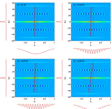
modulated (frequency 2Kd) and not modulated parts. Figure 1 represents the projection of the Wigner function in the phase space domain with u=50 for an equivalent propagation distances of Z=0, Z=0.1Zt, Z=Zt,/4 and Z=Zt,/2 where Zt is the normalized Talbot distance Zt=zt/zc=4π/u² with zt=4πk0/Kd2. For a better visualization, we choose a modulation depth m=0.5.

On the left part and the bottom of each graphic, we have represented respectively the functions W(Kx) and W(X)=F(X) of the

W(X,Kx) function integrated over X and Kx respectively. In the dimensionless phase-space (X,Kx), the Wigner function is composed of one central contribution (centered in Kx=0) and of two lateral contributions at frequency Kd/2, spatially modulated along X with alternatively positive and negative values [28,29]. The thin dashed lines represent the linear curves X=0 and X=2π/u. The thick dashed line represents the displacement of the maxima of the Wigner phase-space function on the lateral contributions. As mentioned in Part 3.A, the odd contributions Kx=±u/2 are composed of cross-terms only and have no energy while even contributions Kx=0,±u are a combination of self and cross-Wigner terms with energy given by the self-terms only. Fig. 1. Phase-space representation of the Talbot effect with five contributions for Gaussian beams for u=50 and m=0.5. On the left of each figure is represented the spatial spectrum (integration over X), and on the bottom, is represented the spatial profile (integration over Kx). The case Ζ=0 represents the beam spatially-phase modulated with

no propagation (no spatial fluence modulations). The case Ζ=0.1Zt

represents a propagation over a fraction of the Talbot distance. The case Ζ=0.25Zt presents a maximal spatial modulation, when the shift of

the periodic is half period. When the shift is Ζ=0.5Zt, modulations are

minimized but not cancelled because the finite size of the beam. For Z=0, the sum of the two lateral contributions, obtained by integration on Kx variable, is equal to zero because they are exactly in opposition of phase. The effect of the propagation along z is to shift along X the lateral contributions, but in opposite directions.

For Z=Zt,/4 modulation are in phase and the integration along Kx of the two lateral contributions gives an extremum of modulation along X.

For Z=Zt/2 the modulations are again in opposition and the sum of the lateral contributions becomes zero again. Nevertheless, modulations are not cancelled due to the finite size of the envelope of the beam. The propagation along z implies a displacement of the lateral contributions and also an inclination of each envelope contribution. If we operate the change of variable(X,Kx) → (X’,Kx) with: '= − x X X ZK , (64) the Wigner phase-space function becomes invariant with Z in this new coordinate system. E. Spectral analysis

Integration of the Wigner function in the spatial domain gives the spatial spectrum of the beam (without the common normalization factor of each contribution): 2 2 2 0 2 2 1 2 2 1 2 2 2

1

( ) exp

₂

1

₂

1 exp

₂

1

( )

exp

₈

exp

₂

₂

1

( )

exp

₈

exp

₂

₂

( )

₄

1 exp

₂

n l x x n l x x n l x x n l x

m

u

W

K

K

u

u

W

K

m

K

u

u

W

K

m

K

m

u

W

K

+ = + = + =− + =

⎛

⎛

⎡

⎤

⎞

⎞

⎡

⎤

=

⎢

_⎣

−

_⎦

⎥⎜

⎜

−

⎜

+

_⎣

⎢

−

⎥

_⎦

⎟

⎟

⎟

⎝

⎠

⎝

⎠

⎡

⎤

⎡

⎤

⎛

⎞

=

⎢

−

⎥

⎢

−

⎜

_⎝

+

⎟

_⎠

⎥

⎢

⎥

⎣

⎦

⎣

⎦

⎡

⎤

⎡

⎤

⎛

⎞

= −

⎢

−

⎥

⎢

−

⎜

−

⎟

⎥

⎝

⎠

⎢

⎥

⎣

⎦

_⎣

_⎦

⎛

⎡

⎤

=

+

_⎢

−

_⎥

⎣

⎦

(

)

(

)

2 2 2 2 2

1

exp

₂

1

( )

₄

1 exp

₂

exp

₂

x n l x x

K

u

m

u

W

_{+ =−}

K

K

u

⎧

⎞

⎫

⎪

⎡

₋

₊

⎤

⎪

⎨

⎜

⎟

_⎢

_⎥

⎬

⎣

⎦

⎪

⎝

⎠

⎪

⎩

⎭

⎧

⎛

⎡

⎤

⎞

⎫

⎪

⎡

⎤

⎪

=

⎨

⎜

+

⎢

−

⎥

⎟

⎢

_⎣

−

−

⎥

_⎦

⎬

⎣

⎦

⎪

⎝

⎠

⎪

⎩

⎭

. (65) The spatial spectrum is independent of the normalized propagation distance Z. Assuming u2_{>>1 (i.e. more than one fringe in the beam), we} get exp(-u2_{)≈0 and terms in m disappear because they correspond to} odd terms. The expression reduces to the three Gaussian contributions centered at Kx=0 (signal without modulations, proportional to W0(Kx)) and Kx=±u (noise), with a weight in m². This result was expected because a convergent description of the beam requires five contributions, with a development at the second order with the modulation depth m (terms in m²):

(

)

(

)

2 2 2 2 2 1 exp ₂ 1 ₂ ( ) 1 1 exp exp 4 2 2 x Seq x x x m K W K m _{K u K u} ⎧ ⎡₋ ⎤⎛ ₋ ⎞ ⎫ ⎪ ⎢_⎣ ⎥_⎦⎜ ⎟ ⎪ ⎪ ⎝ ⎠ ⎪ ≈ ⎨ ⎬ ⎧⎛ ⎡ ⎤ ⎡ ⎤⎞⎫ ⎪_{+ ⎨ − − + − + ⎬}⎪ ⎜ ⎢ ⎥ ⎢ ⎥⎟ ⎪ _{⎩⎝ ⎣ ⎦ ⎣ ⎦⎠⎭}⎪ ⎩ ⎭ . (66) This expression gives a good description of the spatial spectrum of the beam with central and lateral contributions. F. Fluence expression for five contributions Integration of the Wigner function over the spectral coordinate Kx gives the fluence of the beam. From Table 1, integration of the five contributions of the Wigner function, without approximations and without normalization factors, gives the five contributions of the fluence function: 2 0 2 2 2 2 2 2 2 2 2 1 2 2 1

2

( )

p

1 4

2

2

1

1 exp

cos

2

1 4

1 4

2

₂

₂

₂

( )

exp

cos

1 4

1 4

( )

n l n l n l

X

F

X

ex

Z

m

u Z

Xu

Z

Z

u

u

u

X

Z

Z

u X

Z

F

X

m

Z

Z

F

X

m

+ = + = + =−

⎡

⎤

=

_⎢

−

_⎥

+

⎣

⎦

⎧

⎛

⎡

⎤

⎞

⎫

⎪

⎛

⎞

⎪

× −

_⎨

_⎜

+

_⎢

−

_⎥

_⎜

_⎟

_⎟

_⎬

+

⎝

+

⎠

⎣

⎦

⎪

⎝

⎠

⎪

⎩

⎭

⎡

_⎛

_⎞

⎤

_⎛

_⎛

_⎞

_⎞

+

+

+

⎢

⎜

_⎝

⎟

_⎠

⎥

⎜

⎜

_⎝

⎟

_⎠

⎟

⎢

⎥

=

−

⎜

⎟

+

+

⎢

⎥

⎜

⎟

⎜

⎟

⎢

⎥

_⎝

_⎠

⎣

⎦

= −

(

)

(

)

(

)

2 2 2 2 2 2 2 2 2 2 2 2 2 2 2

2

₂

₂

₂

exp

cos

1 4

1 4

2

( )

exp

4

1 4

2

2

1 exp

cos

1 4

1 4

2

( )

₄

exp

n l n l

u

u

u

X

Z

Z

u X

Z

Z

Z

X uZ

m

F

X

Z

u X uZ

u Z

Z

Z

X uZ

m

F

X

+ = + =−

⎡

_⎛

_⎞

⎤

_⎛

_⎛

_⎞

_⎞

−

+

−

⎢

⎜

_⎝

⎟

_⎠

⎥

⎜

⎜

_⎝

⎟

_⎠

⎟

⎢

−

⎥

⎜

⎟

+

+

⎢

⎥

⎜

⎟

⎜

⎟

⎢

⎥

_⎝

_⎠

⎣

⎦

⎡

₊

⎤

=

⎢

−

⎥

+

⎢

⎥

⎣

⎦

⎧

⎡

⎤

⎡

+

⎤

⎫

⎪

⎪

× +

_⎨

_⎢

−

_⎥

_⎢

_⎥

_⎬

+

+

⎪

⎣

⎦

⎣

⎦

⎪

⎩

⎭

−

=

−

(

)

2 2 2 2 2 2

1 4

2

2

1 exp

cos

1 4

1 4

Z

u X uZ

u Z

Z

Z

⎡

⎤

⎢

⎥

+

⎢

⎥

⎣

⎦

⎧

⎡

⎤

⎡

−

⎤

⎫

⎪

⎪

× +

_⎨

_⎢

−

_⎥

_⎢

_⎥

_⎬

+

+

⎪

⎣

⎦

⎣

⎦

⎪

⎩

⎭

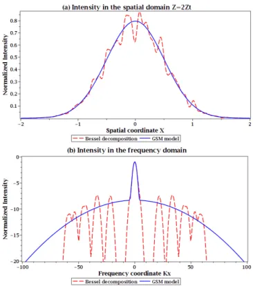
(67) with a total fluence: 0 1 1 2 2 ( ) ( ) ( ) ( ) ( ) ( ). Seq n l n l n l n l n l F X F X F X F X F+ = X + =F+ =− X + = + =− = + + + + (68) This expression contains all the information concerning the Talbot effect coupled with finite pupil and diffraction effects. The fluence formulation consists of three Gaussian waves centered at X0=0,±uZ interacting together with different behavior in different areas [30].

Figure 2 illustrates the evolution of the fluence F(X) with Z (at the left) obtained with the decomposition in Table 2 and the numerical calculation (Beam Propagation Method with 2048x200 points [31]) for a Gaussian beam evolution with Z (at the right) after a phase mask Φ(X)=msin(u) for u=50 and m=0.5. For the numerical calculus, we bring Δx=0.03m and Kd=1666m-1 in the (x,z) coordinates and translate it in (X,Z) coordinates for the comparison with the Bessel decomposition. Fig. 2. Evolution of the normalized fluence with Z for a Gaussian beam: a) Bessel decomposition with five contributions and b) numerical calculus (Beam Propagation Method) for u=50 and m=0.5. Normalized fluence in linear scale.