Is streamflow increasing? Trends in the coterminous United States

(1)

HAL Id: hal-00298936

https://hal.archives-ouvertes.fr/hal-00298936

Submitted on 19 Mar 2008

HAL is a multi-disciplinary open access

archive for the deposit and dissemination of sci-entific research documents, whether they are pub-lished or not. The documents may come from teaching and research institutions in France or abroad, or from public or private research centers.

L’archive ouverte pluridisciplinaire HAL, est destinée au dépôt et à la diffusion de documents scientifiques de niveau recherche, publiés ou non, émanant des établissements d’enseignement et de recherche français ou étrangers, des laboratoires publics ou privés.

Is streamflow increasing? Trends in the coterminous

United States

N. Y. Krakauer, I. Fung

To cite this version:

N. Y. Krakauer, I. Fung. Is streamflow increasing? Trends in the coterminous United States. Hydrol-ogy and Earth System Sciences Discussions, European Geosciences Union, 2008, 5 (2), pp.785-810. �hal-00298936�

(2)

HESSD

5, 785–810, 2008 US streamflow trends N. Y. Krakauer and I. Fung Title Page Abstract Introduction Conclusions References Tables Figures ◭ ◮ ◭ ◮ Back Close

Full Screen / Esc

Printer-friendly Version Interactive Discussion

Hydrol. Earth Syst. Sci. Discuss., 5, 785–810, 2008 www.hydrol-earth-syst-sci-discuss.net/5/785/2008/ © Author(s) 2008. This work is distributed under the Creative Commons Attribution 3.0 License.

Hydrology and Earth System Sciences Discussions

Papers published in Hydrology and Earth System Sciences Discussions are under open-access review for the journal Hydrology and Earth System Sciences

Is streamflow increasing? Trends in the

coterminous United States

N. Y. Krakauer1and I. Fung1,2

1

Department of Earth and Planetary Science, University of California at Berkeley, CA, USA

2

Department of Environmental Science, Policy, and Management, University of California at Berkeley, CA, USA

Received: 12 February 2008 – Accepted: 13 February 2008 – Published: 19 March 2008 Correspondence to: N. Y. Krakauer (niryk@berkeley.edu)

(3)

HESSD

Full Screen / Esc

Printer-friendly Version Interactive Discussion Abstract

An increasing trend in global streamflow has been variously attributed to climate change, land use, and a reduction in plant transpiration under higher CO2 levels. To

separate these influences, we use a subset of ∼1000 United States Geological Sur-vey stream gauges primarily from small, minimally disturbed watersheds to estimate

5

annual streamflow per unit area since 1920 on a uniform grid over the coterminous United States. We find that although streamflow has indeed increased over this pe-riod taken as a whole, this increase has not been uniform in time but concentrated in the late 1960s, when precipitation increased. Since the early 1990s, both precipitation and streamflow show nonsignificant declining trends. Multiple regression of

stream-10

flow against precipitation, temperature and CO₂ suggests that higher CO₂ levels may increase streamflow, presumably due to the physiological plant response to CO2, but

that this positive response is more than offset by the concomitant increasing evapora-tion due to global warming, so that the net impact of greenhouse gas emissions has been to increase evaporation and reduce streamflow. The suppression of plant

transpi-15

ration through higher CO2levels seems to be particularly important for sustaining high

streamflow in recent decades in the Great Plains, where precipitation is concentrated during the growing season.

1 Introduction

Streamflow is important in its own right, as sustaining aquatic life and human water

20

uses, and as a component of the terrestrial water budget. Not surprisingly, several attempts have been made to look in streamflow records for the impact of global warm-ing, other climate variability, and nonclimatic human disturbance, often with an eye to testing models used to predict future changes in the water cycle. Probst and Tardy

(1987,1989) examine discharge records of 50 large rivers, filling in gaps in the records

25

(4)

HESSD

Full Screen / Esc

over 1910–1975 in Africa and the Americas, decreasing streamflow in Europe and Asia, and worldwide a linear trend corresponding to a 3% increase over that period, which they correlate with warming. Labat et al. (2004) analyze runoff records for 221 large rivers, estimating missing values using wavelet transforms. For the periods 1900–1975 (corresponding to Probst and Tardy’s end year) and 1925–1994, they find increasing

5

streamflow in Africa, the Americas, and Asia and decreasing streamflow only in Eu-rope, for a global increase of 3% over 1900–1975 and 8% over 1925–1994, which they propose is evidence for acceleration of the hydrologic cycle caused by global warming; linear regression of runoff on annual global temperature gives a 4% increase per K warming.

10

Gedney et al. (2006) use a land surface model driven by observed climate in an attempt to more rigorously determine the causes for the increased streamflow noted by Labat et al. They find that observed climate changes are insufficient to explain the streamflow increase while changes in land use are modeled to have negligible im-pact on continental or global streamflow. The observed trend can be matched only by

15

including the effect of higher CO2levels in suppressing plant transpiration and thus

in-creasing the share of precipitation that runs off rather than evaporates. Extending this effect into the future,Betts et al.(2007) find that including the favorable impact of high CO2 on streamflow increases projected global streamflow by an amount comparable

to that expected from the climate-induced acceleration of the hydrologic cycle. By

con-20

trast,Piao et al.(2007), simulating 20th century trends in runoff using a different land surface model, find that suppression of transpiration is not necessary to explain the increase found byLabat et al.; in their model, transpiration is not suppressed by higher CO2levels because the increased water use efficiency is offset by faster plant growth

and more leaf area. Instead, they find that land use change, specifically deforestation,

25

can explain much of the observed increase in runoff.

Several studies have examined trends in streamflow in the United States (US), us-ing observations from parts of the extensive United States Geological Survey (USGS) stream gauge network, usually streams from the Hydroclimatic Data Network (HCDN),

(5)

HESSD

Full Screen / Esc

a subset of USGS stream gauges chosen for their long continuous records and mini-mal disturbance of flow due to human land use or water diversions over their periods of measurement (Slack and Landwehr,1992). Lettenmaier et al.(1994) examine trends in monthly streamflow, as well as temperature and precipitation, for 1948–1988, find-ing large increases in cold-season streamflow in the Northeast and Midwest over that

5

period. Lins and Slack (1999) focus on streams with multidecade records that ex-tend through 1993 and find that many streams have shown significantly larger low and medium flows, while high flows do not increase as much.McCabe and Wolock(2002), focusing on the period 1941–1999, find the same pattern of increasing minimum and median annual flow, but point out that the increase took place abruptly around 1970,

10

coincident with an increase in recorded precipitation, and that therefore the increasing trend cannot be confidently extrapolated into the future.

In the work presented here, our aims were (1) to use available streamflow observa-tions to map annual streamflow departures for the coterminous US for as long a period as possible; (2) to evaluate trends in annual streamflow over the coterminous US; and

15

(3) to correlate deduced changes in streamflow with climate variables and with CO2

concentrations. To control for the effects of land use change on streamflow, which may be a significant contributor to recent trends according toPiao et al.(2007), we employ only records from HCDN stations, which primarily represent minimally disturbed small watersheds.

20

2 Methods

2.1 Estimation of gridded streamflow

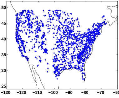
As constructed bySlack and Landwehr(1992), HCDN contains 1659 stream gauges, of which 1571 are in the coterminous United States (distribution shown in Fig.1) and the reminder in Alaska, Hawai’i, Puerto Rico, and the Virgin Islands. Slack and Landwehr

25

(6)

HESSD

Full Screen / Esc

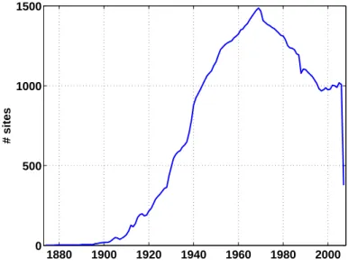
water years, which we updated from USGS through 2007. (USGS defines a water year as extending from October of the previous calendar year through September of the cur-rent year.) The average station has 55 years with complete daily streamflow records (allowing average annual streamflow to be calculated), with fewer station records avail-able before the 1940s (Fig.2).

5

Most of the streams in HCDN drain small watersheds (median drainage area: 740 square km; 10th–90th percentiles: 73–6800 square km). In interpolating measured annual streamflows onto a grid, we therefore treated them as point measurements on the much larger scale (8×106square km) of the coterminous United States. We began by filling in missing years in the streamflow records from the sites that were available

10

for a given year by regularized multiple linear regression (Schneider,2001). This ap-proach provides estimates of the uncertainty of the filled-in missing values, as well as estimates of the mean and covariance of the streamflow records that take into account information from multiple overlapping, correlated records. The streamflow records were normalized by subtracting the long-term mean from each series and dividing by its

15

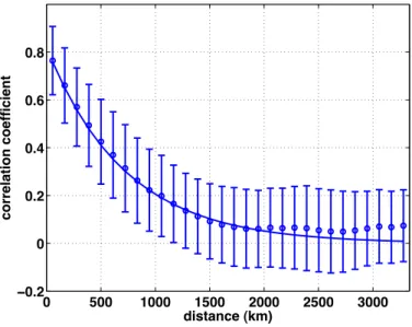
standard deviation. We then fit a two-parameter spatial covariance model (Handcock

and Stein, 1993) to the streamflow series using a restricted maximum likelihood ap-proach (Kitanidis, 1995). The correlation length of streamflow anomalies was found to be about 720 km (Fig.3) and correlation decayed exponentially with distance, con-sistent with other analyses of the spatial correlation of streamflow (Lettenmaier et al.,

20

1994). (For simplicity, we approximated the spatial correlation as homogenous and isotropic. This is not exactly the case; for example, correlelogram analysis showed that the correlation length was about 50% greater in the east than in the more mountainous west and about 40% greater in the east-west compared with the north-south direction.) Each stream record was assigned an error which includes the estimated uncertainty

25

in the series mean and standard deviation, the estimated uncertainty of the filled-in values, and a constant error term intended to represent measurement error and sub-gridscale flow variability whose magnitude (0.06 standard deviations) was determined by restricted maximum likelihood. Finally, given the spatial covariance and error

(7)

struc-HESSD

Full Screen / Esc

ture, each year’s normalized streamflow at the gauge locations was interpolated, as in the standard geostatistical (“Kriging”) approach (Cressie,1993), to a 1◦ grid covering the coterminous United States. The gridded normalized streamflows were scaled by gridded mean and interannual standard deviation of streamflow per unit area from the analysis ofFekete et al.(2002) to produce estimates of actual streamflow per unit area

5

(in mm/yr) for each water year.

2.2 Climate and greenhouse-gas concentration data

We sought to correlate streamflow anomalies to anomalies in local precipitation, large-scale temperature (not local temperature, because this can be strongly influenced by precipitation variations as well as influencing them) and atmospheric CO2 concentra-10

tion. We used gridded precipitation from the Global Historical Climatology Network (GHCN) Version 2, which is based on quality-controlled station observations over land processed to provide the best representation of long-term variability (Peterson and

Vose, 1997, http://www.ncdc.noaa.gov/oa/climate/research/ghcn/ghcngrid.html). To get more accurate ratios of streamflow to precipitation, we downscaled the precipitation

15

amounts from the 5◦ resolution of GHCN to the 1◦resolution of our grid using climato-logical gridded precipitation from the University of East Anglia’s Climate Research Unit (CRU; New et al.,1999,http://www.cru.uea.ac.uk/cru/data/hrg/cru ts 2.10/), multiply-ing the GHCN time series for each grid cell by a scalar representmultiply-ing the ratio in the CRU climatology between the precipitation at 1◦ resolution and that at 5◦ resolution.

20

Hemispheric and global monthly temperature anomalies were also taken from CRU (Jones and Moberg,2003,http://cdiac.esd.ornl.gov/trends/temp/jonescru/jones.html). Yearly atmospheric CO2 concentrations were estimated from direct measurements at

Mauna Loa since the late 1950s and from ice core measurements beforehand (Enting

et al.,1994).

(8)

HESSD

Full Screen / Esc

3 Results

3.1 Streamflow trends and their correlation with precipitation

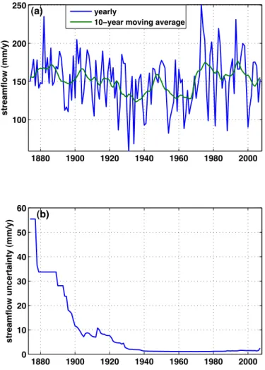
Figure4shows estimated annual streamflows for the coterminous United States, along with their uncertainty as estimated from the covariance and error structures of the HCDN records. This uncertainty was large in the first few decades, because there

5

weren’t enough records to accurately delineate patterns in annual streamflows (Fig.2). We restricted our analysis of trends in streamflow to the period since 1920, when the streamflow gauge network appears to be dense enough to allow for accurate year-by-year reconstruction of large-scale streamflow patterns. (The estimated uncertainty shown in Fig. 4b does not include that introduced by scaling with the the analyzed

10

mean and standard deviation from Fekete et al. (2002). This source of uncertainty, while difficult to quantify, would be expected to affect primarily our estimate of the absolute amount of streamflow and not its interannual variability.) We found periods of low streamflow in the 1930s and 1950s–1960s, and high streamflow in the 1970s and 1980s. A linear least-squares trendline of estimated streamflows over 1925–1994

15

supports Labat et al.’s (2004) finding of increasing streamflow in North America over this period: the regression coefficient is +0.57±0.22 mm/yr per year (p=0.03 for the null hypothesis of a regression coefficient of zero, using the F-test with the number of degrees of freedom adjusted for series autocorrelation (Bretherton et al.,1999)). How-ever, the increase over this period mostly took place abruptly around 1970, rather than

20

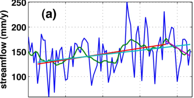
continuing steadily through recent decades. In fact, over the period 1994–2007, i.e. subsequent to that covered inLabat et al.’s analysis, streamflow shows a nonsignifi-cant decreasing trend of−2.3±2.2 mm/yr (p=0.48) (Fig.5a).

As recognized by McCabe and Wolock (2002) for minimum and median annual streamflows, long-term trends in mean streamflow were well correlated with trends

25

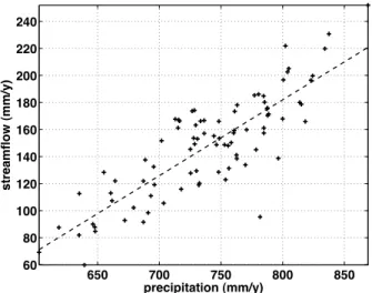
in precipitation, which also shows an abrupt increase around 1970 followed by essen-tially no trend since then (Fig.5b). High-frequency interannual fluctuation in precipita-tion was also matched by fluctuaprecipita-tions in streamflow. In fact, as Fig.6shows, most of

(9)

HESSD

Full Screen / Esc

the streamflow variability could be explained by a linear dependence on current-year precipitation (R2_=0.70).

Our gridded streamflow product permits us to compare not only trends in stream-flow and precipitation averaged over the coterminous US but also spatial patterns in streamflow with spatial patterns in precipitation at comparable effective resolution over

5

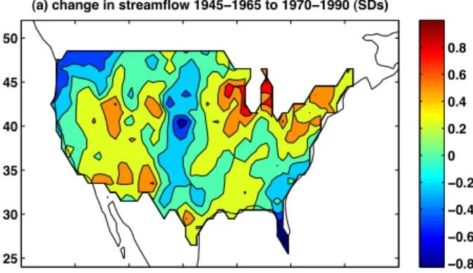
particular time periods. As an example, Fig. 7 shows maps of interdecadal change in streamflow and precipitation. Between 1945–1965 and 1970–1990, precipitation in-creased over most of the US, with a particularly pronounced increase in the northeast, but decreased over Florida and the northwest. Between 1970–1990 and 1995–2007 precipitation increased in the upper Great Plains and northern California but decreased

10

in the Rocky Mountain region and in the southeast. In both cases, streamflow shows quite similar trends.

Annual streamflow correlated well with annual precipitation throughout most of the coterminous US (Fig. 8). This dependence was weakest in the Great Plains, where precipitation is concentrated in the summer and only a small fraction runs off, so that

15

the timing of rainfall and the antecedent soil moisture status may be relatively more important to determining streamflow than the annual total, and strongest in the moist east and the Pacific coast.

3.2 Impact of global warming and atmospheric CO₂on streamflow

While the major direct cause of interannual variability in streamflow is variability in

20

precipitation, changing temperature and CO₂ level might also be expected to affect streamflow, the former through influencing evaporation rates, and the latter by affecting plant water use efficiency. In an attempt to isolate the impact on streamflow of global warming and of increasing ambient CO₂ levels, we performed multiple linear regres-sion of streamflow against annual precipitation, temperature, and CO2 level. We cau-25

tion that because global temperature is well correlated with CO2 levels, linear

regres-sion has limited ability to distinguish the separate effects of these two factors. For the coterminous US we found opposing impacts of temperature and CO2 in the expected

(10)

HESSD

Full Screen / Esc

directions, with warming reducing streamflow while higher CO₂ increases streamflow (Table1).

Since (greenhouse) warming and rising CO2have been well correlated and are likely

to remain so in coming decades, a possibly more important question is the net effect of the combination of high CO2 and warming. Regression of streamflow against pre-5

cipitation and CO2 alone showed that the overall effect of greenhouse warming has

probably been to reduce streamflow, though the association is not significant for the coterminous US as a whole (Table1).

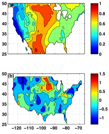
The dependence of streamflow on global temperature and CO2 level varied by

re-gion (Fig. 9b). CO₂ seems relatively most influential in increasing streamflow in the

10

Great Plains, while in the east, with its wetter conditions, and in the far west, with its concentration of winter precipitation, the positive impact of CO2 on streamflow is less

strong than the negative impact of warming. Dividing the coterminous United States based on the percentage of precipitation that falls during the warm months shows this division clearly (Fig.9a; Table1).

15

4 Discussion

4.1 Is greenhouse warming causing the observed increase in streamflow?

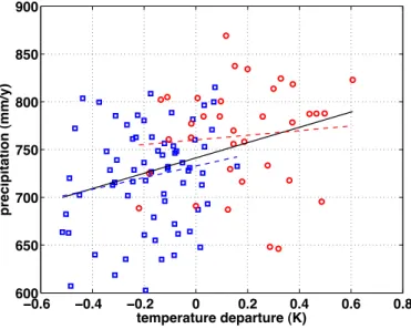
Figure 10 shows coterminous United States precipitation versus global temperature for each year in 1901–2005. While the two time series show a nominally significant positive correlation of +0.35 (p<0.001) because the higher precipitation after 1970

cor-20

responds to warmer global temperatures, segmenting the time series at 1970 shows that the correlation is mostly due to the abrupt jump in precipitation around 1970 rather than a more consistent trend (correlation for 1901–1970 +0.19, for 1970–2005 +0.09, both with p>0.05). This jump in precipitation has been tentatively linked with chang-ing circulation patterns in the Atlantic Ocean, possibly reinforced by increaschang-ing aerosol

25

(11)

HESSD

Full Screen / Esc

response of coterminous United States precipitation to global temperature in the ob-servational record.

Absent a direct effect of greenhouse warming on coterminous US precipitation, most of the US shows a negative impact of greenhouse warming on streamflow, which could be explained through the increased evaporation due to global warming more than

off-5

setting the increased plant water use efficiency due to higher CO2 concentrations.

While separating the temperature from the CO₂impacts based on observational data is uncertain because both these factors are increasing over time in a similar manner, our multiple regression of streamflow against temperature and CO2 level provides some

support for the contention ofGedney et al.(2006) that a direct CO₂impact on

stream-10

flow is detectable. Our inference that total evaporation nevertheless is increasing with warming is consistent with in situ measurements of evaporation (Golubev et al.,2001). We found that the apparent CO2 impact on streamflow is strongest in parts of the

United States where summer precipitation dominates. This pattern agrees with the ex-pectation that the impact of increased plant water use efficiency on streamflow should

15

be largest where precipitation is concentrated during the growing season and therefore is efficiently intercepted by plants, as opposed to where much precipitation occurs in winter so that growing-season transpiration has a relatively smaller impact on stream-flow (Wigley et al.,1984).

4.2 What do observed trends suggest about future moisture regimes?

20

Our results show that fitting a linear trend to streamflow (or precipitation) data can be highly misleading for understanding decadal variability and for extending observed patterns into the future. While coterminous United States streamflow and precipitation have indeed increased in recent decades, this increase took place abruptly over a few years around 1970, rather than as part of a steady “acceleration of the hydrologic

25

cycle” in step with greenhouse gas concentrations or global warming. Thus, there is no clear reason to expect continued increases in streamflow with greater warming. If precipitation follows its post-1970 trend and fails to increase with additional warming,

(12)

HESSD

Full Screen / Esc

we should expect streamflow to continue to decrease over most of the United States, as it has since the early 1990s, due to intensified evaporation (incompletely offset by the physiological impact of CO2on plants). Indeed, increasing drought over the United

States since the early 1990s is proposed to have caused a reduction in the summer drawdown of atmospheric CO2observed at Mauna Loa, as water stress reduced plant 5

carbon uptake during the growing season (Buermann et al.,2007). The global trend since the 1970s has also been toward more frequent drought occurrence (Dai et al.,

2004). Extending our work through objective interpolation of streamflow trends in other regions where many long records are available would help give a clearer picture of how decadal hydrologic variability and the effects of greenhouse warming on the water

10

cycle vary between continents and biomes.

Considering only annual mean streamflow and precipitation may not be sufficient for understanding how water stress and water resource availability have changed and may change. For example, part of the increase in streamflow observed in the Great Plains that our regression analysis attributed to increasing atmospheric CO2could in-15

stead be due to reduced interannual precipitation variability (Garbrecht and Rossel,

2002) or to a disproportionate increase in cold-season (as compared with summer) precipitation (Garbrecht et al., 2004). Our interpolation technique could equally well be applied to seasonal or monthly as well as annual mean streamflow, and thus dis-tinguish the hydrologic impacts of these as well as other seasonally specific factors as

20

advances in spring snowmelt and changing vegetation phenology. It is also important to examine how changes in precipitation intensity (Groisman et al.,2001) might also affect streamflow and other aspects of the water cycle. Comparing trends in gridded streamflow from a larger gauge network with the trend estimated using HCDN could independently validate model assessments of the impact on streamflow of human land

25

use and water diversion, whereas in this study we chose to obtain trend estimates that exclude land use impacts insofar as possible. Finally, combining gridded streamflow and precipitation with remotely sensed water storage would give a fuller picture of how climate variability is affecting stored soil water and groundwater.

(13)

HESSD

Full Screen / Esc

5 Conclusions

We developed maps of annual streamflow anomalies over the coterminous United States. We find that streamflow increased around 1970 in concert with an increase in precipitation, but has not increased since then. Our analysis supports net drying as a result of greenhouse warming, with some evidence for the opposing effects of

tem-5

perature and CO₂ increase. This suggests a high risk of reduced water supplies and increased plant water stress with continued warming in coming decades.

Acknowledgements. N. Y. Krakauer thanks NOAA for a Climate and Global Change

Postdoc-toral Fellowship. I. Fung acknowledges support from NOAA Office of Global Programs, Award NA05OAR4311167. We thank A. Alkhaled, A. Michalak and K. Mueller for geostatistics help,

10

B. Fain, J. Hunt and T. Pagano for proofreading and useful suggestions, and G. Farquhar, C. Pathak, M. Roderick and R. Teegavarapu for valuable comments.

References

Baines, P. G. and Folland, C. G.: Evidence for a rapid global climate shift across the late 1960s, J. Climate, doi:10.1175/JCLI4177.1, 2007.793

15

Betts, R., Boucher, O., Collins, M., Cox, P., Falloon, P., Gedney, N., Hemming, D., Hunting-ford, C., Jones, C., Sexton, D., et al.: Projected increase in continental runoff due to plant responses to increasing carbon dioxide., Nature, 448, 1037–41, 2007. 787

Bretherton, C. S., Widmann, M., Dymnikov, V. P., Wallace, J. M., and Blad ´e, I.: The effective number of spatial degrees of freedom of a time-varying field, J. Climate, 12, 1990–2009,

20

1999. 791

Buermann, W., Lintner, B. R., Koven, C. D., Angert, A., and Pinzon, J. E.: The changing carbon cycle at Mauna Loa Observatory, Proc. Natl. Acad. Sci., 104, 4249–4254, 2007.795 Cressie, N. A.: Statistics for Spatial Data, Wiley, revised edn., 1993.790

Dai, A., Trenberth, K. E., and Qian, T.: A global data set of Palmer Drought Severity Index for

25

1870-2002: Relationship with soil moisture and effects of surface warming, J. Hydrometeo-rol., 5, 1117–1130, 2004. 795

(14)

HESSD

Full Screen / Esc

Enting, I., Wigley, T. M. L., and Heimann, M.: Future Emissions and Concentrations of Car-bon Dioxide: Ocean/Atmosphere/Land Analyses, Technical Paper no. 31, CSIRO Division of Atmospheric Research, 1994. 790

Fekete, B. M., V ¨or ¨osmarty, C. J., and Grabs, W.: High resolution fields of global runoff com-bining observed river discharge and simulated water balances, Global Biogeochem. Cy., 16,

5

1042, doi:10.1029/1999GB001254, 2002. 790,791

Garbrecht, J., Liew, M. V., and Brown, G. O.: Trends in precipitation, streamflow, and evap-otranspiration in the Great Plains of the United States, J. Hydrol. Eng., 9, 360–367, doi: 10.1061/(ASCE)1084-0699(2004)9:5(360), 2004.795

Garbrecht, J. D. and Rossel, F. E.: Decade-scale precipitation increase in Great Plains at end of

10

20th century, J. Hydrol. Eng., 7, 64–75, doi:10.1061/(ASCE)1084-0699(2002)7:1(64), 2002. 795

Gedney, N., Cox, P. M., Betts, R. A., Boucher, O., Huntingford, C., and Stott, P. A.: Detection of a direct carbon dioxide effect in continental river runoff records, Nature, 439, 835–838, doi:10.1038/nature04504, 2006. 787,794

15

Golubev, V., Groisman, P., Speranskaya, N., Zhuravin, S., Menne, M., Peterson, T., and Mal-one, R.: Evaporation changes over the contiguous United States and the former USSR: A reassessment, Geophys. Res. Lett., 28, 2665–2668, 2001. 794

Groisman, P. Y., Knight, R. W., and Karl, T. R.: Heavy precipitation and high streamflow in the contiguous United States: Trends in the Twentieth Century, B. Am. Meteorol. Soc., 82,

20

219–246, 2001. 795

Handcock, M. S. and Stein, M. L.: A Bayesian analysis of kriging, Technometrics, 35, 403–410, 1993. 789

Jones, P. D. and Moberg, A.: Hemispheric and large-scale surface air temperature variations: An extensive revision and an update to 2001, J. Climate, 16, 206–223, 2003.790

25

Kitanidis, P. K.: Quasi-linear geostatistical theory for inversing, Water Resour. Res., 31, 2411– 2420, 1995. 789

Labat, D., Godderis, Y., Probst, J. L., and Guyot, J. L.: Evidence for global runoff increase related to climate warming, Adv. Water Resour., 27, 631–642, 2004.787,791

Lettenmaier, D. P., Wood, E. F., and Wallis, J. R.: Hydro-climatological trends in the continental

30

United States, 1948–88, J. Climate, 7, 586–607, 1994. 788,789

Lins, H. F. and Slack, J. R.: Streamflow trends in the United States, Geophys. Res. Lett., 26, 227–230, doi:10.1029/1998GL900291, 1999.788

(15)

HESSD

Full Screen / Esc

McCabe, G. J. and Wolock, D. M.: A step increase in streamflow in the conterminous United States, Geophys. Res. Lett., 29, 2185, doi:10.1029/2002GL015999, 2002.788,791

New, M., Hulme, M., and Jones, P.: Representing twentieth-century space-time climate vari-ability – Part I: Development of a 1961–90 mean monthly terrestrial climatology, J. Climate, 12, 829–856, 1999.790

5

Peterson, T. C. and Vose, R. S.: An overview of the Global Historical Climatology Network temperature data base, B. Am. Meteorol. Soc., 78, 2837–2849, 1997. 790

Piao, S., Friedlingstein, P., Ciais, P., de Noblet-Ducoudre, N., Labat, D., and Zaehle, S.: Changes in climate and land use have a larger direct impact than rising CO₂on global river runoff trends, Proc. Natl. Acad. Sci., 104, 15 242–15 247, doi:10.1073/pnas.0707213104,

10

2007. 787,788

Probst, J. L. and Tardy, Y.: Long range streamflow and world continental runoff fluctuations since the beginning of this century, J. Hydrol., 94, 289–311, doi:10.1016/0022-1694(87) 90057-6, 1987. 786,787

Probst, J.-L. and Tardy, Y.: Global runoff fluctuations during the last 80 years in relation to world

15

temperature change, Am. J. Sci., 289, 267–285, 1989. 786

Schneider, T.: Analysis of incomplete climate data: Estimation of mean values and covari-ance matrices and imputation of missing values, J. Climate, 14, 853–871, doi:10.1175/ 1520-0442(2001)014h0853:AOICDEi2.0.CO;2, 2001. 789

Slack, J. R. and Landwehr, J. M.: Hydro-Climatic Data Network (HCDN): A U.S. Geological

Sur-20

vey Streamflow Data Set for the United States for the Study of Climate Variations, 1874-1988, Tech. rep., USGS Open-File Report 92-129,http://pubs.usgs.gov/wri/wri934076/, 1992.788 Wigley, T. M. L., Briffa, K. R., and Jones, P. D.: Atmospheric carbon dioxide: Predicting plant productivity and water resources, Nature, 312, 102–103, doi:10.1038/312102a0, 1984. 794

(16)

HESSD

Full Screen / Esc

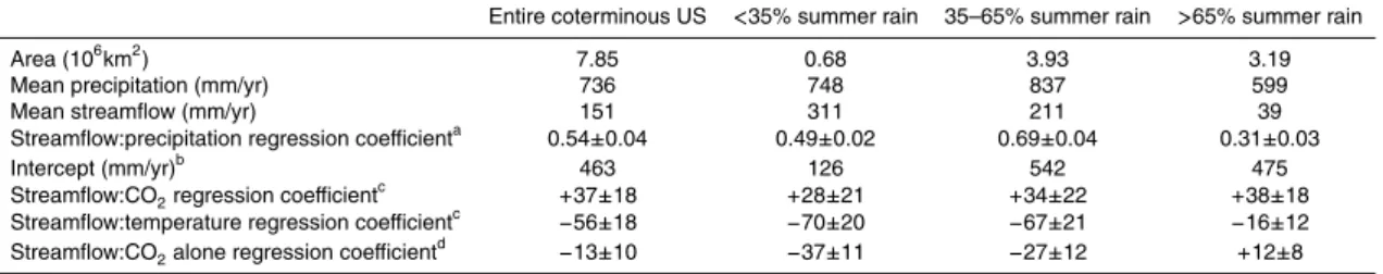
Table 1. Streamflow variability by precipitation seasonality and for the entire coterminous US

Entire coterminous US <35% summer rain 35–65% summer rain >65% summer rain

Area (106km2) 7.85 0.68 3.93 3.19

Mean precipitation (mm/yr) 736 748 837 599

Mean streamflow (mm/yr) 151 311 211 39

Streamflow:precipitation regression coefficienta _0.54±0.04 _0.49±0.02 _0.69±0.04 _0.31±0.03

Intercept (mm/yr)b 463 126 542 475

Streamflow:CO2regression coefficientc +37±18 +28±21 +34±22 +38±18

Streamflow:temperature regression coefficientc −56±18 −70±20 −67±21 −16±12 Streamflow:CO2alone regression coefficientd −13±10 −37±11 −27±12 +12±8 a

For a regression of streamflow against precipitation alone (coefficient is unitless, mm/yr per mm/yr).

b

Precipitation at zero streamflow (a measure of “baseline” plant transpiration and evaporative demand).

c

For a regression of streamflow against precipitation, temperature, and CO2level

(coefficients expressed as mm/yr streamflow per 100 ppm CO2and mm/yr streamflow per K, respectively). d

(17)

HESSD

Full Screen / Esc

Printer-friendly Version Interactive Discussion −130 −120 −110 −100 −90 −80 −70 −60 25 30 35 40 45 50

(18)

HESSD

Full Screen / Esc

Printer-friendly Version Interactive Discussion 1880 1900 1920 1940 1960 1980 2000 0 500 1000 1500 # sites

Fig. 2. HCDN sites with complete discharge records per water year. (The drop for the most

(19)

HESSD

Full Screen / Esc

Printer-friendly Version Interactive Discussion 0 500 1000 1500 2000 2500 3000 !0.2 0 0.2 0.4 0.6 0.8 distance (km) c o rr e la ti o n c o e ffi c ie n t

Fig. 3. Inter-gauge correlation of annual streamflow, binned in 110-km bins. Error bars show

standard deviation of the correlation coefficient within each bin. The curve is an exponential-decay fit with a scale length of 720 km.

(20)

HESSD

Full Screen / Esc

Printer-friendly Version Interactive Discussion 1880 1900 1920 1940 1960 1980 2000 100 150 200 250 s tr e a m fl o w (m m /y ) (a) 1880 1900 1920 1940 1960 1980 2000 0 10 20 80 40 50 60 s tr e a m fl o w u n c e rta in ty (m m /y ) (b) yearly

10!year moving average

Fig. 4. (a) Estimated yearly streamflow for the coterminous United States, along with a 10-yr

(21)

HESSD

Full Screen / Esc

Printer-friendly Version Interactive Discussion 100 150 200 250 s tr e a m fl o w (m m /y )

_(a)

1920 1940 1960 1980 2000 650 700 750 800 850 p re c ip ita ti o n (m m /y )

(b)

Fig. 5. (a) Estimated yearly streamflow for the coterminous United States since 1920, with

a 10-yr moving average and least-squares trendlines for 1925–1994, 1925–2007, and 1994– 2007. (b) Yearly precipitation for the coterminous United States since 1920 with a 10-yr moving average.

(22)

HESSD

Full Screen / Esc

Printer-friendly Version Interactive Discussion 650 700 750 800 850 60 80 100 120 140 160 180 200 220 240 precipitation (mm/y) s tr e a m fl o w (m m /y )

Fig. 6. Yearly coterminous United States streamflow ploted against precipitation, 1920–2005. The linear regression trendline is also drawn: streamflow=(0.54± 0.04)×precipitation−(248±28) mm/yr.

(23)

HESSD

Full Screen / Esc

(a) change in streamflow 1945!1965 to 1970!1990 (SDs)

25 30 35 40 45 50 !0.8 !0.6 !0.4 !0.2 0 0.2 0.4 0.6 0.8 (b) change in precipitation 1945!1965 to 1970!1990 (SDs) !130 !120 !110 !100 !90 !80 !70 !60 25 30 35 40 45 50 !1 !0.5 0 0.5 1

Fig. 7. (a–b) Change in average streamflow and precipitation between 1945–1965 and 1970–

1990 (later period minus earlier period). (c–d) Same, but between 1970–1990 and 1995–2007 (1995–2005 for precipitation). Changes have been normalized by the interannual standard deviation at each point so that changes in wet and dry regions have comparable magnitude.

(24)

HESSD

Full Screen / Esc

Printer-friendly Version Interactive Discussion (c) change in streamflow 1970!1990 to 1995!2007 (SDs) 25 30 35 40 45 50 (d) change in precipitation 1970!1990 to 1995!2007 (SDs) !130 !120 !110 !100 !90 !80 !70 !60 25 30 35 40 45 50 !1 !0.5 0 0.5 1 !1 !0.5 0 0.5 1 Fig. 7. Continued.

(25)

HESSD

Full Screen / Esc

Printer-friendly Version Interactive Discussion (a) 25 30 35 40 45 50 0 0.2 0.4 0.6 0.8 1 (b) !120 !100 !80 25 30 35 40 45 50 0.2 0.4 0.6 0.8

Fig. 8. (a) Regression coefficient on precipitation of annual streamflow, 1920–2005

(dimen-sionless, mm/yr per mm/yr). (b) Fraction of interannual variability in streamflow explainable by linear regression on annual precipitation (R2).

(26)

HESSD

Full Screen / Esc

Printer-friendly Version Interactive Discussion (b) !120 !110 !100 !90 !80 !70 25 30 35 40 45 50 (a) 25 30 35 40 45 50 0 0.2 0.4 0.6 0.8 1 !1 !0.5 0 0.5 1 1.5

Fig. 9. (a) Summer dominance of precipitation, defined as the fraction of climatological annual

precipitation that falls during warmer than average months of the year. (b) Apparent response of streamflow to greenhouse warming: the regression coefficient of CO2level on annual

stream-flow in a multiple regression of streamstream-flow against precipitation and CO₂ (so that the effect of global warming is implicitly included in the CO₂term). Units are streamflow standard deviations per 100 ppm CO₂. The standard error of the regression coefficient is about 0.3 SD/100 ppm CO₂.

(27)

HESSD

Full Screen / Esc

Printer-friendly Version Interactive Discussion !0.6 !0.4 !0.2 0 0.2 0.4 0.6 0.8 600 650 700 750 800 850 900 temperature departure (K) p re c ip ita ti o n (m m /y )

Fig. 10. Annual global temperature and coterminous US precipitation, 1901–2005. Blue

squares are years from 1901–1970, red circles are years from 1971–2005. The solid line is the least-squares regression line for the entire period, while the blue and red dashed lines are regression lines for the periods 1901–1970 and 1970–2005, respectively. While over the whole period precipitation is significantly, if weakly, correlated with temperature (R2_{=0.12), the} correlation vanishes after 1970.