HAL Id: hal-02377790
https://hal.archives-ouvertes.fr/hal-02377790
Submitted on 24 Nov 2019
HAL is a multi-disciplinary open access
archive for the deposit and dissemination of
sci-entific research documents, whether they are
pub-lished or not. The documents may come from
teaching and research institutions in France or
abroad, or from public or private research centers.
L’archive ouverte pluridisciplinaire HAL, est
destinée au dépôt et à la diffusion de documents
scientifiques de niveau recherche, publiés ou non,
émanant des établissements d’enseignement et de
recherche français ou étrangers, des laboratoires
publics ou privés.
Size invariance of the granular Rayleigh-Taylor
instability
Jan Vinningland, Øistein Johnsen, Eirik Flekkøy, Renaud Toussaint, Knut
Jørgen Måløy
To cite this version:
Jan Vinningland, Øistein Johnsen, Eirik Flekkøy, Renaud Toussaint, Knut Jørgen Måløy. Size
in-variance of the granular Rayleigh-Taylor instability. Physical Review E : Statistical, Nonlinear, and
Soft Matter Physics, American Physical Society, 2010, 81 (4), �10.1103/PhysRevE.81.041308�.
�hal-02377790�
Size invariance of the granular Rayleigh-Taylor instability
Jan Ludvig Vinningland,1,2,
*
Øistein Johnsen,1 Eirik G. Flekkøy,1Renaud Toussaint,3and Knut Jørgen Måløy1 1Advanced Materials and Complex Systems, Department of Physics, University of Oslo, P.0. Box 1048, 0316 Oslo, Norway 2
Physics of Geological Processes, Department of Physics, University of Oslo, P.0. Box 1048, 0316 Oslo, Norway 3
Institut de Physique du Globe de Strasbourg, CNRS, Université Louis Pasteur, 5 rue Descartes, 67084 Strasbourg Cedex, France
共Received 3 September 2008; revised manuscript received 18 February 2010; published 29 April 2010兲
The size scaling behavior of the granular Rayleigh-Taylor instability关J. L. Vinningland et al., Phys. Rev. Lett. 99, 048001 共2007兲兴 is investigated experimentally, numerically, and theoretically. An upper layer of grains displaces a lower gap of air by organizing into dense fingers of falling grains separated by rising bubbles of air. The dependence of these structures on the system and grain sizes is investigated. A spatial measurement of the finger structures is obtained by the Fourier power spectrum of the wave number k. As the size of the grains increases the wave number decreases accordingly which leaves the dimensionless product of wave number and grain diameter, dk, invariant. A theoretical interpretation of the invariance, based on the scaling properties of the model equations, suggests a gradual breakdown of the invariance for grains smaller than ⬃70 m or greater than ⬃570 m in diameter.
DOI:10.1103/PhysRevE.81.041308 PACS number共s兲: 81.05.Rm, 47.20.Ma, 47.11.⫺j, 45.70.Qj
I. INTRODUCTION
Granular materials are the basis of abundant industrial and natural processes and an integral part of our everyday life. Dry granular flows have been widely studied over the past twenty years 关1兴, but the study of granular flows where the interstitial fluid plays an important role is still in its infancy. Many natural phenomena pertaining to such granular/fluid flows are active topics of current research, e.g., sedimenta-tion 关2,3兴, erosion and river evolution 关4兴, underwater ava-lanches and turbidites关5兴, and soil fluidization during earth-quakes关6兴. Industrial processes, such as pneumatic transport, fluidized beds, catalytic cracking 关1,7,8兴 would also benefit from advances in granular/fluid flow research.
The granular Rayleigh-Taylor instability arises when a closed, vertical Hele-Shaw cell, partially filled with fine grains and air at atmospheric pressure, is rapidly rotated to bring the dense packing of grains above a layer of air. Shortly after the rotation fine fingers of falling grains emerge from the initially flat grain-air interface. These fine fingers subsequently develop into coarser finger structures separated by bubbles of air. In contrast to the classical Rayleigh-Taylor instability关9兴 the coarsening process observed in the granu-lar case will right from the start bring about a reduction in the number of fingers and a corresponding increase in the size of the bubbles. New fingers will form in the center of the rising bubbles as they reach a certain width, and the charac-teristic size of the structures is thus maintained at a stable value.
This granular instability is previously studied both nu-merically and experimentally关10,11兴, using the same model and setup as in the present paper, with the conclusion that the two competing mechanisms, one producing finer scales, the other producing coarser scales, are well reproduced by the numerical model.
In contrast to the gas-grain instability reported here, Völtz
et al. studied a liquid-grain instability experimentally and
theoretically关12兴. The liquid-grain instability bears a strong resemblance to the classical instability for two liquids with almost overlapping dispersion relations. The gas-grain insta-bility, however, displays a quite different behavior with a coarsening process active from the beginning and a counter-acting refinement process that stabilizes the average size of the bubbles.
The purpose of the present investigation is to study the variations in the flow structures under change of spatial scale of both the grains and the Hele-Shaw cell. Size invariance is not commonly studied for granular materials. Indeed, granu-lar flows are quite sensitive to initial preparation and external perturbations, so that systematic grain and system size changes are delicate studies. In the present paper, using the complementarity of experimental and numerical techniques, we perform a systematic study of how the structures formed by the granular Rayleigh-Taylor instability responds to a res-caling of the system and grain sizes.
The experimental, numerical, and theoretical results pre-sented all indicate a size invariance of the finger-bubble structures. However, the theoretical analysis predicts a break-ing of the invariance if the grains are too small or too large. The simulations use grains ranging from 70 to 490 m in diameter, and the experiments use grains ranging from 80 to 570 m in diameter. Consistent data collapses are obtained from these results and demonstrate a fairly robust invariance within the given limits.
The simulations and experiments presented in Ref. 关11兴 were performed with identical parameters to provide an as-sessment of the numerical model. In the present paper we present experimental and numerical results obtained in a new parameter regime not explored in previous publications. However, in this paper the parameters of the experiments and simulations are no longer identical, due to less emphasis on model assessment. In particular, the simulations and experi-ments are carried out using slightly different grain densities. The scale invariance of the granular Rayleigh-Taylor invari-ance was first acknowledged in Ref.关10兴. The current paper provides a more elaborate discussion of this invariance in-*janlv@fys.uio.no
cluding results from experiment, simulation and theory not presented in关10兴.
The paper is organized as follows. A presentation of the experimental setup and implementation is given in the next section. The numerical model is briefly presented in Sec.III, and the results, together with the data analysis, are presented and discussed in Sec. IV. The theoretical basis of the size invariance, based on the scaling properties of the model equations, is presented in Sec. V. Section VI presents nu-merical data obtained to check for possible container size effects. Finally, a conclusion and summary are given in Sec. VII.
II. EXPERIMENT
The experimental setup is the same as was used in Refs. 关10,11兴 and will only be presented briefly here. Four Hele-Shaw cells of different sizes are partially filled with mono-disperse polystyrene beads and air at atmospheric pressure. The sizes of the cells scale proportionally with the diameter of the grains they contain, see Table I. The cells are filled with Dynoseeds polystyrene spheres of density
g= 1.05 g/cm3 共manufactured by Microbeads 关13兴兲. The
cells are individually mounted on a hinged bar and rapidly rotated to an upright position, see Fig.1. Images of the fall-ing grains are recorded by a high speed digital camera 共Photron Fastcam-APX 120K兲 at a rate of 500 frames per second.
The humidity in the laboratory was kept at about 30% during the assembling of the cells, and the grains were ex-posed to the air in the laboratory for some time before the
filling. This is to prevent clustering of the grains due to co-hesion, arising from capillary bridges, or electrostatic forces. The experimental cells are somewhat taller than the nu-merical cells to account for the grains that settle during the rotation. The horizontal filling procedure of the cells makes it difficult to control the filling fraction, and it may vary slightly between the four cells. During the assembling of the cells the TS 500–53 beads was presumed to have a diameter of 500 m. However, an analysis performed by Microbeads shows that the mean diameter of these grains is in fact 570 m. This explains the slight discrepancy between the width of the cell and the diameter of the grains in this case.
III. SIMULATION
The numerical model has proved to be very consistent in reproducing experimentally observed structures in granular flows and instabilities in the regime of low Reynolds num-bers 关14–17兴. The theoretical basis and derivation of the model are given in Refs. 关14,15兴 and a description of the current implementation is given in Ref. 关11兴. However, a brief outline of the model will be presented here for com-pleteness.
The granular phase is modeled as discrete, rigid spheres that collectively constitute a deformable porous medium. The pressure drop associated with the air flowing through the granular medium is given by a local Darcy’s law关18兴 with the Carman-Kozeny relation for the permeability关19兴. The continuum gas phase is described solely by its pressure P. The velocity field of the gas may be obtained from the pres-sure gradient via Darcy’s law. In order to provide a con-tinuum description of the pressure P共x,y兲 on a grid 共x,y兲, the continuum variables, solid fraction 共x,y兲, and granular ve-locity u共x,y兲 need to be calculated. This is done by a linear smoothing function s共r−r0兲 expressed mathematically as 关14兴 s共r − r0兲 =
冦
冉
1 −⌬x l冊冉
1 − ⌬y l冊
if ⌬x,⌬y ⬍ l 0 otherwise,冧
共1兲 where r共x,y兲 is the position of the grain, r0共x0, y0兲 is the position of the grid node, ⌬x=兩x−x0兩 and ⌬y=兩y−y0兩 are the relative distances, l is the lattice constant, and 兺ks共r−rk兲=1 with k indexing the four neighboring sites of agrain positioned at r.
From the continuity equations of air mass and grain mass, using the average velocity of the air in the porous matrix 共i.e., uDarcy/兲, a pressure equation is derived, see 关14,15兴,
冉
Pt + u ·P
冊
= ·冉
P 共兲 P
冊
− P · u, 共2兲where= 1 − is the porosity, and is the viscosity of air. This equation is valid for compressible flows since it as-sumes a⬀P 共isothermal ideal gas law兲 for the air density, a. If instead an incompressible liquid is considered this
as-sumption becomesl⬀for the liquid densityl. The
pres-sure Eq. 共2兲 then simplifies to a Poisson equation for the pressure given by·关共兲/ P兴=·u.
TABLE I. Listing of the diameters of the grains and the dimen-sions of the Hele-Shaw cells used in the experiments.
Diameter 共m兲 80 140 230 570 Width共mm兲 31 56 91 200 Height共mm兲 61 86 141 305 Depth共mm兲 1.0 1.7 2.3 5.4 befor e rotation after
rotation stoppingbar
silicone frame falling grains rising air-bubble new finger new bubble
FIG. 1.共Color online兲 共left兲 Side view of the experimental setup with the initial and final cell positions superimposed.共right兲 Typical snapshot from an experiment using grains of 230 m in diameter in a cell that is 91⫻141⫻2.3 mm.
VINNINGLAND et al. PHYSICAL REVIEW E 81, 041308共2010兲
The grains are governed by Newton’s second law
mdv
dt = mg + FI−
V P
, 共3兲
where m, v, and V are, respectively, the mass, velocity, and volume of a grain. The interparticle normal force FI acting between grains in contact is calculated iteratively using con-tact dynamics关20兴 共but a Hookean or Hertzian contact law may be used instead兲. The dynamics of the grains are sim-plified by neglecting particle-particle and particle-wall fric-tion. A lower cutoff is imposed on the solid fraction because the Carman-Kozeny relation is not valid for a solid fraction less than 0.25关21兴. This cutoff causes the permeability in the most dilute regions of the system to be slightly underesti-mated. This leads to a slight overestimation of the pressure forces acting on grains in dilute regions. The effect of this artifact is however decreasing with increasing granular iner-tia.
A series of seven simulations are performed and each simulation uses monodisperse grains of different diameters, see TableII. The same relative start configuration of 160 000 grains is used in all the simulations and the size of the sys-tem, given in TableII, scales proportionally to the diameters of the grains. The mass density of the grains is 2.5 g/cm3, a common value for glass beads. In the simulations we have introduced a larger density than in the experiments in order to minimize the numerical artifacts caused by the solid
frac-tion cutoff. These artifacts are manifested as slightly curved and buckled fingers that become visible as the inertia of the grains decreases.
IV. RESULTS AND ANALYSIS
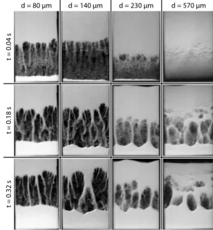
Images from each of the seven simulations and four ex-periments are, respectively, shown in Figs.2and3. The cor-responding spatial dimensions of the cells are given in Tables I andII. Each row of images in Figs. 2 and3 represents a given time t, and each column of images represents a given grain-diameter d. From the snapshots in Figs. 2 and3 it is evident that the finger-bubble structures depend strongly on grain size. For cells with grains of diameters smaller than
TABLE II. Listing of the diameters of the grains and the dimen-sions of the cells used in the simulations.
Diameter 共m兲 70 140 210 280 350 420 490 Width共mm兲 28 56 84 112 140 168 196 Height共mm兲 34 68 102 136 170 204 238 d = 70 μm d = 140 μm d = 210 μm d = 280 μm d = 350 μm d = 420 μm d = 490 μm t = 0.06 s t = 0.14 s t = 0.22 s
FIG. 2. Numerical snapshots. Each column represents different simulations using grains of diameter d, and each row represents snapshots at different times t. d = 80 μm t = 0.04 s d = 570 μm d = 230 μm d = 140 μm t = 0.32 s t = 0.18 s
FIG. 3. Experimental snapshots. Each column represents a dif-ferent experiment characterized by the diameter d of the grains used, and each row represents a different time t.
200 m it is relatively easy to identify a unique interface that separates an upper, dense granular packing from the air below. For grain diameters greater than 200 m, however, small air-bubbles appear in the bulk of the packing above the grain-air interface. These precursory bubbles are separated by horizontal filaments of grains which form in addition to the vertical fingers. The number of precursory bubbles in-creases as the grain diameter inin-creases. These structures are analogous to the bubbles observed in the ripple instability arising in a tilted tube of sand 关16,22兴.
Scale invariance
A size measurement of the finger structures is obtained by making a Fourier transform of the solid fraction field共x,y兲. The resulting Fourier spectrum S¯共k,t兲, i.e., the wave number distribution for a given time t, enables a quantitative com-parison of finger structures for different grain and system sizes.
The distribution S¯共k,t兲 is calculated as follows. The power spectrum Sj共k兲 of each horizontal line j of the solid
fraction field is obtained by the discrete Fourier transform 关23兴, using Hamming data windows to avoid frequency leak-age due to the nonperiodic character of the system. By aver-aging over the individual power spectra Sj共k兲 the final
aver-age distribution S¯共k,t兲 is obtained. This procedure is illustrated in Fig.4: the left plot shows power spectra Sj共k兲
obtained at three given positions yj of horizontal cuts of the
density function 共x,y兲 shown in the right plot of the same figure. Largevalues appear in red共gray兲 and smallvalues appear in blue共dark gray兲.
As Fig.4illustrates it is not necessary to reduce the Fou-rier analysis to a spatial window centered around the face. The power spectra obtained in the bulk above the inter-face are anyway flat and make no contributions to the final averaged power spectrum.
The experimental data are treated similarly to the numeri-cal data. However, the solid fraction field is not directly available in the experimental data and it is therefore esti-mated by the gray level values of the image pixels. The pixel value is assumed to be linearly related to the solid fraction. The inaccuracy of this assumption is not likely to have a large effect on the measurements.
Figure 5 shows log-log plots of S¯共dk兲, i.e., the power spectra S¯共k兲 rescaled by the grain-diameter d, for the numeri-cal data. The inset plots show the unsnumeri-caled spectra S¯共k兲 as function of k in cm−1. Notice that the power spectra in Fig.5 k (1/cm) Sj (k) y 0 4 8 12 x (cm) 0 1 2 3 4 5
FIG. 4.共Color online兲 Plots of Fourier power spectra Sj共k兲 共left兲 obtained at three different heights of the solid fraction field共x,y兲 共right兲 shown as a color coded data image 关red 共gray兲 is high, blue 共dark gray兲 is low 兴. The stapled white lines indicate at which y position the power spectra are obtained.
10−2 10−1 10−2
10−1 100 101
(grain diameter)x (wave number)
S( d k) a) t = 0.06 s 10−1 100 101 10−2 100 10−2 10−1 10−2 10−1 100 101
(grain diameter)x (wave number)
S( d k) b) t = 0.14 s (dk)−2.5 10−1 100 101 10−2 100 10−2 10−1 10−2 10−1 100 101
(grain diameter)x (wave number)
S( d k) c) t = 0.22 s 10−1 100 101 10−2 100 increasing diameter incr easing diameter increasing diameter (dk)−2.5
FIG. 5. 共Color online兲 Plots of S¯共dk兲 关S¯共k兲 in inset plots兴 ob-tained from numerical data. Each plot is a data collapse of S¯共dk兲 for all grain-diameters d at three different times t共the same times as in Fig. 2兲. The different colors represent different grain diameters
ranging from 70 to 490 m as indicated in the inset plots. The straight black lines are power laws obeyed by S¯共dk兲 at large and small scales: S¯共dk兲⬃constant at large scales 共growing white noise兲, and S¯共dk兲⬃共dk兲−2.5at small scales.
VINNINGLAND et al. PHYSICAL REVIEW E 81, 041308共2010兲
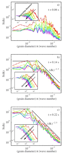
are calculated from the numerical data shown in Fig.2. Fig-ure 6 similarly shows log-log plots of S¯共dk兲 obtained from the experimental data presented in Fig. 3. The inset plots show the unscaled spectra S¯共k兲.
The plot in Fig.5共a兲hardly qualifies as a data collapse, in contrast to the other plots in Figs.5and6. This is due to the fact that initially the falling grains are constantly expanding which increases the divergence of the velocity field,·u. As is shown in Eq.共8兲 the source term, P ·u, of the pressure equation Eq.共2兲 will break the invariance. Hence, the invari-ance observed for larger times is only possible due to the
smallness of the source term for larger times.
The characteristic wave number共where the power spectra start to decrease兲 seen in Fig.5 gradually shifts from higher to lower values as time evolves. This corresponds well with the observed coarsening with time of the finger structures both in the numerical and the experimental data. However, compared to the numerical data, the shift from higher to lower wave numbers is less evident in the experimental data since the initially very fine fingers is not observed in the experiments.
After the very initial period, the共collapsed兲 power spectra plotted in Figs. 5and6 can be shown to be consistent with two power laws: S¯共dk兲⬃constant for large scales 共growing white noise兲, and S共dk兲⬃共dk兲−2.5 at small scales 共straight black lines in Figs. 5 and 6兲. These exponents can be ob-tained from linear fits of the bilogarithmic plots, and are determined with a precision of order 0.5. These power laws are valid both for the numerical 共Fig. 5兲 and experimental 共Fig.6兲 results. In the experiments, however, there is also an additional bump of the power spectra for the smallest scales 共largest wave numbers兲 departing from the S共dk兲⬃共dk兲−2.5 scaling behavior. This behavior may be attributed to the fact that these largest k values are at the limit of the spatial res-olution in the experiments.
The early-time power spectra displayed in Figs. 5共a兲and 6共a兲are quite scattered around the power laws. This might be related to the fact that at early times the size scaling is also not satisfied due to accelerating grains, as previously dis-cussed.
V. THEORETICAL INTERPRETATION
Let us assume that we have a solution of our gas and grain equations. Now, if we magnify all physical scales, the veloci-ties and the pressure variations by a constant factor , how close will we come to a solution of our equations?
In mathematical terms, let P,共x,t兲=mn共x,t兲, and vibe
the pressure field, the mass density field, and particle veloci-ties that solve the equations
dP dt = ·
冉
P P 冊
− P · u, mdv dt = mg + FI− m P , 共4兲where as before u is the local average of the vi’s. We split the
velocity as follows: vi=␦vi+ u0 and u =␦u + u0, where u0 is the constant sedimentation velocity of a close packed system. We substitute P = P0+␦P and FI= maIand make the
observa-tion that ␦PⰆ P0, which leads to the justified approximation
␦P t = ·
冉
P0␦P 冊
− P0 ·␦u, dv dt = g + aI− P . 共5兲Here the substantial derivative has been replaced by the par-tial derivative because u ·␦PⰆ P0 ·␦u. A rough estimate
10−2 10−1 104 105 106 107 a) t = 0.04 s
(grain diameter)x (wave number)
S(dk) 10−1 100 101 104 106 10−2 10−1 104 105 106 107 b) t = 0.18 s
(grain diameter)x (wave number)
S(dk) 10−1 100 101 104 106 10−2 10−1 104 105 106 107 c) t = 0.32 s
(grain diameter)x (wave number)
S(dk) 10−1 100 101 104 106 (dk)−2.5 (dk)−2.5 incr easing diameter increasing diameter increasing diameter
FIG. 6. 共Color online兲 Plots of S¯共dk兲 关S¯共k兲 in inset plots兴 ob-tained from experimental data. Each plot is a data collapse of S¯共dk兲 for all grain-diameters d at three different times t共the same times as in Fig.3兲. The different colors represent different grain diameters
ranging from 80 m to 570 m as indicated in the inset plots. The straight black lines are power laws obeyed by S¯共dk兲 at large and small scales, as in the numerical case: S¯共dk兲⬃constant at large scales, and S¯共dk兲⬃共dk兲−2.5at small scales.
using u⬃10−2 m/s, ␦P⬃10−3 Pa/m, P
0= 105 Pa, and ·␦u⬃10 s−1 justifies this assumption. As in a hydrostatic system we assume that the pressure field of the magnified system is␦P
⬘
共x⬘
, t兲=␦P共x,t兲=␦P共x⬘
/,t兲, where x⬘
=x. We make the following scaling ansatz, expressing the solu-tions of Eqs.共5兲 in terms of the scaled fields as␦P共x,t兲 =1 ␦P
⬘
共x⬘
,t兲, u0= 1 2u0⬘
, ␦u共x,t兲 =1 ␦u⬘
共x⬘
,t兲, 共x,t兲 =⬘
共x⬘
,t兲, 共6兲where the sedimentation velocity u0
⬘
scales as2because the local density is -invariant and permeability goes as length squared and scales as 2, i.e.,
⬘
=2. 共7兲Note that Eqs.共5兲 are unaffected by the scaling of u0. Using the new length scale in the derivative
⬘
we get =⬘
. The pressure gradient␦P, ,, and t are all invariant. By substitution we obtain ␦P⬘
t =⬘
·冉
⬘
P0⬘
␦P⬘
冊
−P0⬘
·␦u⬘
, 1 冉
dv⬘
dt − aI⬘
冊
= g − ⬘
P⬘
⬘
, 共8兲as the equations satisfied by the scaled fields. Note that by mass conservation of the granular phase, i.e.,
d/dt=− ·␦u, the last term of the pressure equation may
be written −P0 ·␦u =共P0/兲d/dt, and this term thus gives the effect of density changes in a frame of reference moving with the grains. This implies that the term vanishes for a flow field without internal compression or expansion. If such a flow field is also steady, like that of a slab of connected particles moving at a constant velocity, the acceleration terms vanish along with the −P0 ·␦u term, i.e., all the -dependent terms vanish in Eq. 共8兲. This invariance means that the scaled fields are solutions of the same equations as the original fields.
The terms that are multiplied by a -factor break the in-variance. To get an estimate of their relative magnitude we introduce dimensionless numbers. Taking the characteristic length scale of the flow to be l and the time scale to be l/u we may write Fr =u 2 gl⬃ dv/dt g , A =180 ul ␦Pd2 ⬃ P0 ·␦u ·
冉
P0␦P 冊
, 共9兲where Fr is known as the Froude number. Taking
d = 140 m, l =具k典−1= 0.01 m at t = 0.5 s and
u = l/t=0.02 m/s we get Fr=0.004. With␦P = 0.01 atm. and
the same values for the length scale l we get A = 0.04. Since A and Fr measure the relative magnitude of the invariance-breaking terms, the smallness of A and Fr indicate that the scaled fields are close to satisfying the physical Eqs. 共5兲. For this reason we may expect all lengths in the simula-tions to scale the same way, and S¯共dk兲 will be invariant under scaling by . However, since Fr⬀, increasing the magnifi-cation will increase the relative effect of granular inertia, and, we expect, the deviations from this scaling property. On the other hand, A⬀1/ so decreasing the particle size will cause the compression term in the pressure equation to grow in relative magnitude. It is therefore only in a certain window of particle sizes around d = 140 m that we may expect the scale invariance. In particular, for the d = 70 m simulations it is likely that deviations from the scaling behavior arise due to the relatively large A value.
The above scaling invariance is somewhat analogous to the scale invariance of low Reynolds number flows, where
0 0.1 0.2 0.3 0.4 0.5 0 1 2 3 4 5 6
(a)
time (s) < k > (1/cm) w = 14 mm w = 28 mm w = 42 mm w = 56 mm 0 0.1 0.2 0.3 0.4 0.5 0 1 2 3 4(b)
time (s) σ k (1 /cm ) w = 14 mm w = 28 mm w = 42 mm w = 56 mmFIG. 7. 共Color online兲 共a兲 Plot of the mean wave number 具k典 obtained from four different simulations with grains of diameter
d = 140 m but with four different cell widths w. 共b兲 Same plot for
the standard deviation.
VINNINGLAND et al. PHYSICAL REVIEW E 81, 041308共2010兲
the inertial term may be neglected since it is small compared to the viscous term, and symmetries of the flow solutions emerge because the Navier-Stokes equations are replaced by the Stokes equation.
VI. CONTAINER SIZE EFFECTS
In the experiments and simulations presented so far the size of the grains and the size of the container are changed proportionally to each other such that every container con-fines approximately the same number of grains. To address the question of possible container size effects a series of simulations is performed where the size of the grains and the size of the container are changed independently. Four differ-ent simulation geometries are used while the grain diameter is kept fixed at 140 m. The four numerical cells all have the same height of 68 mm but different widths of 14, 28, 42, and 56 mm. To compare the different results the power spec-trum S¯共k,t兲 for each of the four simulations is obtained as explained in Sec.IV. In order to represent the temporal evo-lution of S¯共k,t兲 the mean and standard deviation of S¯共k,t兲 are calculated by the usual definitions
具k典共t兲 =
兺
kS¯共k,t兲兺
¯共k,t兲S , 共10兲 共t兲 =冑
兺
k 2¯共k,t兲S兺
¯共k,t兲S −具k典共t兲2, 共11兲 where the summation is over all k values.Figure 7 shows the mean wave number具k典 and standard deviation for the four different geometries. During the coarsening stage, i.e., from t = 0 s until t = 0.2 s, the four curves overlap quite well. For t⬎0.2 s the curves are more
spread due to two peaks in the w = 14 and 28 mm data. These peaks are most likely caused by fluctuations in the evolving structures which are not averaged out due to less statistics for the narrow geometries. In addition, the different granular configurations used in the four runs also account for some variations in the data. For cell widths less than roughly 14 mm container size effects will be present since this width is smaller than the maximum width a bubble may reach in a wide cell. However, the data in Fig. 7 shows no systematic dependence on the container size.
In 关10兴 it was shown that plots of 具k典 for different grain sizes will overlap only if 具k典 is rescaled by the grain-diameter d. In Fig.7the plots overlap although no rescaling of 具k典 by, e.g., the container width w is applied. Hence, the observed pattern scales with grain size and not container size.
VII. CONCLUSION AND SUMMARY
In summary we have uncovered an approximate scale in-variance in a granular Rayleigh-Taylor instability 关10,11兴 through experimental measurements and complementary simulations. In addition, a theoretical interpretation is pro-vided with the conclusion that the validity of the scale in-variance is limited to a window of grain diameters from roughly 70 m to about 570 m. The scale invariance may be interpreted as the existence of a Stokes-like regime for the investigated systems. Terms arising from grain inertia for large grains, or from pressure sources共i.e., P ·u兲 for small grains, will gradually break the invariance. A separate series of simulations with constant grain sizes but different geom-etries was performed with the conclusion that the observed scale invariance is not affected by container size effects. The deviations observed in this invariance has been given inter-pretations both in terms of theoretical arguments and in terms of numerical and experimental imperfections.
关1兴 Physics of Dry Granular Media, edited by H. J. Herrmann, J.-P. Hovi, and S. Luding, NATO ASI Series E: Applied Sci-ences Vol. 350 共Kluwer Academic Publishers, Dordrecht, 1998兲.
关2兴 G. K. Batchelor,J. Fluid Mech. 52, 245共1972兲.
关3兴 J. F. Richardson and W. N. Zaki, Trans. Inst. Chem. Eng. 3, 65 共1954兲.
关4兴 P. Y. Julien, River Mechanics 共Cambridge University Press, Cambridge, 2002兲.
关5兴 D. H. Rothman, J. P. Grotzinger, and P. B. Flemings, J. Sedi-ment Res. 64, 59共1994兲.
关6兴 R. Bachrach, A. Nur, and A. Agnon,J. Geophys. Res. 106, 13515共2001兲.
关7兴 J. F. Davidson and D. Harrison, Fluidization 共Academic Press, New York, 1971兲.
关8兴 D. Gidaspow, Multiphase Flow and Fluidization 共Academic Press, San Diego, 1994兲.
关9兴 G. Taylor,Proc. R. Soc. London, Ser. A 201, 192共1950兲.
关10兴 J. L. Vinningland, Ø. Johnsen, E. G. Flekkøy, R. Toussaint,
and K. J. Måløy,Phys. Rev. Lett. 99, 048001共2007兲.
关11兴 J. L. Vinningland, Ø. Johnsen, E. G. Flekkøy, R. Toussaint, and K. J. Måløy,Phys. Rev. E 76, 051306共2007兲.
关12兴 C. Völtz, W. Pesch, and I. Rehberg,Phys. Rev. E 65, 011404 共2001兲.
关13兴 Microbeads AS, P. O. Box 265, N-2021 Skedsmokorset, NOR-WAY, Tel:⫹47 64 83 53 00, Fax: ⫹47 64 83 53 01, email: support@micro-beads.com.
关14兴 S. McNamara, E. G. Flekkøy, and K. J. Måløy,Phys. Rev. E
61, 4054共2000兲.
关15兴 D.-V. Anghel, M. Strauss, S. McNamara, E. G. Flekkøy, and K. J. Måløy,Phys. Rev. E 74, 029906共E兲 共2006兲.
关16兴 E. G. Flekkøy, S. McNamara, K. J. Måløy, and D. Gendron,
Phys. Rev. Lett. 87, 134302共2001兲.
关17兴 Ø. Johnsen, R. Toussaint, K. J. Måløy, and E. G. Flekkøy,
Phys. Rev. E 74, 011301共2006兲.
关18兴 H. Darcy, Les Fontaines Publiques de la Ville de Dijon 共Dal-mont, Paris, 1856兲.
关20兴 F. Radjai, M. Jean, J.-J. Moreau, and S. Roux,Phys. Rev. Lett.
77, 274共1996兲.
关21兴 A. A. Zick and G. M. Homsy,J. Fluid Mech. 115, 13共1982兲.
关22兴 D. Gendron, H. Troadec, K. J. Måløy, and E. G. Flekkøy,
Phys. Rev. E 64, 021509共2001兲.
关23兴 W. H. Press, S. A. Teukolsky, W. T. Vetterling, and B. P. Flan-nery, Numerical Recipes in C⫹⫹: The Art of Scientific
Com-puting 共Cambridge University Press, Cambridge, 2002兲, p.
505, Chap. 12.
VINNINGLAND et al. PHYSICAL REVIEW E 81, 041308共2010兲