HAL Id: hal-01702549
https://hal.archives-ouvertes.fr/hal-01702549
Submitted on 20 Dec 2019
HAL is a multi-disciplinary open access
archive for the deposit and dissemination of
sci-entific research documents, whether they are
pub-lished or not. The documents may come from
teaching and research institutions in France or
L’archive ouverte pluridisciplinaire HAL, est
destinée au dépôt et à la diffusion de documents
scientifiques de niveau recherche, publiés ou non,
émanant des établissements d’enseignement et de
recherche français ou étrangers, des laboratoires
The expressiveness of quasiperiodic and minimal shifts
of finite type
Bruno Durand, Andrei Romashchenko
To cite this version:
Bruno Durand, Andrei Romashchenko. The expressiveness of quasiperiodic and minimal shifts of
finite type. Ergodic Theory and Dynamical Systems, Cambridge University Press (CUP), 2021, 41
(4), pp.1086-1138. �10.1017/etds.2019.112�. �hal-01702549�
arXiv:1802.01461v5 [cs.DM] 26 Nov 2019
The expressiveness of quasiperiodic and minimal
shifts of finite type
∗
Bruno Durand and Andrei Romashchenko
November 27, 2019
Abstract
We study multidimensional minimal and quasiperiodic shifts of finite type. We prove for these classes several results that were previously known for the shifts of finite type in general, without restriction. We show that some quasiperiodic shifts of finite type admit only non-computable con-figurations; we characterize the classes of Turing degrees that can be rep-resented by quasiperiodic shifts of finite type. We also transpose to the classes of minimal/quasiperiodic shifts of finite type some results on sub-dynamics previously known for the effective shifts without restrictions: every effective minimal (quasiperiodic) shift of dimension d can be rep-resented as a projection of a subdynamics of a minimal (respectively, quasiperiodic) shift of finite type of dimension d + 1.
Keywords: minimal SFT; quasiperiodicity; tilings
1
Introduction
In this paper we study the multi-dimensional shifts, i.e., the shift-invariant and topologically closed sets of configurations in Zd over a finite alphabet. The min-imal shifts are those shifts in which all configurations contain exactly the same finite patterns; the quasiperiodic shifts are the shifts where each configuration contains all of its finite patterns infinitely often, at least once in every large enough region.
Two classes of shifts play a prominent role in symbolic dynamics, in language theory, and in the theory of computability: the shifts of finite type (obtained by forbidding a finite number of finite patterns) and the effective shifts (obtained by forbidding a computable set of finite patterns).
The class of shifts of finite type is known to be very rich — even a finite set of simple local rules can induce a rather sophisticated global structure. It is known that some (non-empty) multi-dimensional shifts of finite type admit
∗Supported by the ANR grant Racaf ANR-15-CE40-0016-01. Preliminary versions of some
of the presented results we published in conference papers on MFCS-2015 [23] (Theorems 3-4) and MFCS-2017 [26] (Theorems 6-7).
only aperiodic (see [1]) or even only non-computable ([3, 4]) configurations. The value of the combinatorial entropy of a shift of finite type can be any right computable real number h ≥ 0, see [17]. Recent results (see [15, 19, 20]) show that if we look at the projective subdynamics of a shift of finite type of some dimension d > 1, we can obtain any effective shift of a dimension below d.
The proofs of the results mentioned above are based on embedding some computation in the structure of a shift of finite type. These embedding use rather tricky combinatorial gadgets that permit marrying the ‘computational’ techniques with the framework of symbolic dynamics. Though the implied com-putational tricks may look natural to a computer scientist, they give in the end constructions that are rather complex and artificial if we look at them as objects of dynamical systems theory.
Thus, a natural question is whether the phenomena mentioned above hold for ‘simpler’ and ‘more natural’ shifts of finite type. A formal version of this problem is to transpose some results known for shifts of finite type in general to some sort of primary shifts. More technically, in this paper we deal with minimal, quasiperiodic, and transitive shifts. Our results can be subdivided into three groups:
• We prove that some quasiperiodic shifts of finite type admit only non-computable configurations. Moreover, we characterize the classes of Tur-ing degrees that may correspond to a quasiperiodic shift of finite type. • We transpose the characterization by Hochman and Meyerovitch of the
entropies of multidimensional shifts of finite type to the class of transitive shifts. (The same result was recently proven by Gangloff and Sablik in [25] with a different technique.)
• We extend to the classes of minimal/quasiperiodic shifts of finite type some known results on subdynamics: every effective minimal (quasiperiodic) shift of dimension d can be represented as a projection of a subdynamics of a minimal (respectively, quasiperiodic) shift of finite type of dimension d + 1, which answers positively a question by E. Jeandel, [22]
All constructions in this paper involve the technique of self-simulating tilings developed in [19] (see also variants of this technique in [24, 28]).
1.1
Notation and basic definitions
Shifts. Let Σ be a finite set (an alphabet). Fix an integer d > 0. A Σ-configuration (or just a Σ-configuration if Σ is clear from the context) on Zd is
a mapping f : Zd → Σ, i.e., a coloring of Zd by “colors” from Σ. A Zd
-shift (or just a -shift ) is a set of configurations that is (i) translation invariant (with respect to the translations along each coordinate axis), and (ii) closed in Cantor’s topology.
If a Zd-shift S
1 is subset of a Zd-shift S2, we say that S1 is a subshift of
S2 The entire space ΣZ
d
is itself a shift (where no pattern is forbidden) and is called the full shift. Thus, every Zd-shift is a subshift of the full shift.
A pattern is a mapping from a finite subset of Zd to Σ (a coloring of a finite
set of Zd); this set is called the support of the pattern. We say that a pattern P
appears in a configuration f (¯x) if for some ¯c ∈ Zd the pattern P coincides with
the restriction of the shifted configuration fc¯(¯x) := f (¯x + ¯c) to the support of
this pattern. A pattern that appears in some configuration of a shift is called globally admissible.
Every shift is determined by the corresponding set of forbidden finite pat-terns F (a configuration belongs to the shift if and only if no patpat-terns from F appear in this configuration).
A shift is called effective (or effectively closed ) if it can be defined by a computably enumerable set of forbidden patterns. A shift is called a shift of finite type (SFT) if it can be defined by a finite set of forbidden patterns.
Wang tilings. A special class of two-dimensional SFT is defined in terms of Wang tiles. In this case, we interpret the alphabet Σ as a set of tiles, i.e., a set of unit squares with colored sides, assuming that all colors belong to some finite set C (we assign one color to each side of a tile, so technically Σ is a subset of C4). A (valid) tiling is a set of all configurations f : Z2→ Σ where every two
neighboring tiles match, i.e., share the same color on adjacent sides. Wang tiles are powerful enough to simulate any SFT in a very strong sense: for each SFT S there exists a set of Wang tiles τ such that the set of all τ -tilings is isomorphic to S. In this paper we mainly use the formalism of tilings since Wang tiles are better adapted for explaining our techniques of self-simulation.
Dynamics and subdynamics. Every shift S ⊂ ΣZd
can be interpreted as a dynamical system. Indeed, there are d translations along the coordinate axes, and each of these translations maps S to itself. Therefore, the group Zdnaturally
acts on S.
Let S be a shift on Zdand L be k-dimensional sub-lattice in Zd(i.e., L must be an additive subgroup of Zd that is isomorphic to Zk). Then the L-projective subdynamics SL of S is the set of configurations of S restricted on L. The
L-projective subdynamics of a Zd-shift can be understood as a Zk-shift (note that
L naturally acts on SL). In particular, for every d′< d we have a Zd
′
-projective subdynamics on the shift S, generated by the lattice on the first d′ coordinate
axis.
A configuration x is called recurrent if every pattern that appears in x at least once, must then appear in this configuration infinitely often.
A shift S is called transitive if there exists a configuration x ∈ S that contains every finite pattern that appears in at least one configuration y ∈ S.
Quasiperiodicity and minimality. A configuration x is called quasiperiodic (or uniformly recurrent ) if every pattern P that appears in x at least once must appear in every large enough cube Q in x. Note that every periodic configuration is also quasiperiodic. A quasiperiodic shift is a shift that contains only quasiperiodic configurations.
Given a configuration x, a function of a quasiperiodicity for x is a mapping ϕ : N → N ∪ {∞} such that every finite pattern of size (diameter) n either never appears in x or appears in every cube of size ϕ(n) in x (see [8]). We assume ϕ(n) = ∞ if some pattern P of size n appears in x but there exist arbitrarily large areas in x that are free of P . By definition, for a quasiperiodic x we have ϕ(n) < ∞ for all n. We say that a shift S has a function of quasiperi-odicity if there exists a function ϕ(n) (finite for all n) that is a function of a quasiperiodicity for every configuration in S.
A shift is called minimal if it contains no non-trivial subshifts (except the empty set and itself). A shift S is minimal if and only if all its configurations contain exactly the same patterns. If a shift is minimal, then it is quasiperiodic (the converse is not true).
Since each minimal shift S is quasiperiodic, for every minimal shift S there is a function of quasiperiodicity ϕ(n) that is finite for all n. Besides, for an effective minimal shift, the set of all finite patterns (that can appear in any configuration) is computable, see [15, 16]. From this fact it follows that every effective and minimal shift contains some computable configuration. Indeed, with an algorithm that checks whether a given pattern appears in every x ∈ S, we can incrementally (and algorithmically) increase a finite pattern, maintaining the property that this pattern appears in every configuration in S.
Topological entropy. Let Qk be the d-dimensional cube of size k,
Qk := {0, 1, . . . , k − 1}d.
For a shift S in ΣZd
, we denote by NS(k) the number of distinct Σ-colorings of
Qk that appear as a pattern in configurations from S. The topological entropy
of S is defined by
h(S) = lim
k→∞
log NS(k)
|Qk|
with the logarithm to base 2. (The limit above exists for any shift.)
1.2
The main results
The main results of this paper can be subdivided into three groups: construc-tions combining quasiperiodicity with high computational complexity, a con-struction of a transitive SFT with a given topological entropy, and subdynamics of minimal and quasiperiodic SFT. In what follows we state our results more precisely.
1.2.1 Quasiperiodicity is compatible with non-computability
A configuration f : Zd→ Σ, is called periodic if there exists a non-zero c ∈ Zd such that f (x + c) = f (x) for all x. Otherwise a configuration is called aperiodic. In the classic paper [1], Berger came up with a shift of finite type where all configurations are aperiodic.
Theorem 1 (Berger). For every d > 1 there exists a non-empty SFT on Zd
where each configuration is aperiodic.
This construction, as well as a simpler one proposed by Robinson in [2], is quite sophisticated, with tricky combinatorial gadgets embedded in the struc-ture of all configurations of the shift. So the SFT obtained in these seminal papers (and many subsequent constructions elaborating the ideas of Berger and Robinson) look rather messy in terms of dynamical systems. The SFTs pro-posed by Berger and Robinson are not “simple” as a topological object, neither minimal nor transitive1.
Later it was shown that the property of aperiodicity can be enforced for minimal shifts of finite type. In other words, the combinatorial complexity (the property of aperiodicity of an SFT) can be combined with topological simplicity (the property of minimality), as in the following theorem.
Theorem 2 (Ballier–Ollinger). For every d > 1 there exists a non-empty SFT on Zd where each configuration is aperiodic and quasiperiodic (and even
mini-mal ).
(This result was proven in [14] for a tile set τ constructed in [12]. Other ex-amples of minimal aperiodic SFTs were suggested in in [30, 29].) Our next result in some sense strengthens Theorem 2: we claim that there exists a quasiperiodic SFT that contains only non-computable configurations.
Theorem 3. For every d > 1 there exists a non-empty SFT on Zd where all
configurations are non-computable and quasiperiodic.
Note that we cannot strengthen Theorem 3 further and change quasiperiodic-ity to minimalquasiperiodic-ity: in every minimal SFT the set of globally admissible patterns is decidable, and therefore there exists a computable configuration, see [16] and [15].
With a similar technique we prove the following (more general) result, which characterize the classes of Turing degrees that can be represented by quasiperi-odic SFTs.
Theorem 4. For every effectively closed set A and for every d > 1 there exists a non-empty SFT S in Zd where all configurations are quasiperiodic, and the
Turing degrees of all configurations in S form exactly the upper closure of A (defined as the set of all Turing degrees d such that d ≥T x for at least one
x ∈ A).
1
The basic construction of an aperiodic SFT by Robinson admits configurations that consist of two half-planes which can be arbitrarily shifted one with respect to the other. Robinson referred to this phenomenon as a fault in a tiling, see [2, Section 3]. This makes the SFT non-minimal and even non-transitive.
The shifts obtained by enriching the generic construction of Robinson (tilings with embed-ded computations) may be even more irregular. If they admit configurations with potentially different computations (which is unavoidable in some applications), then it is difficult to enforce the appearance in one single configuration of all fragments of computations that po-tentially might appear in at least one valid configuration. Recently several authors proposed nontrivial regularizations of Robinson’s construction overcoming the aforementioned obstacles, see below.
Remark 1. The Turing degree spectrum of a non effective minimal shift can be much more complex than what we get in Theorem 4, see [27].
1.2.2 The Hochman–Meyerovitch theorem on the entropy of SFTs Hochman and Meyerovitch showed in [17] that a real number h ≥ 0 is the topo-logical entropy of some SFT if and only if h is right recursively enumerable. They raised the question whether the same property holds for the class of tran-sitive shifts. Recently Gangloff and Sablik [25] answered this question potran-sitively using a construction based on Robinson’s aperiodic tilings. We prove the same result (Theorem 5 below) using a technique similar to the proof of Theorem 3. Theorem 5. For every integer d > 1 and for every nonnegative right recursively enumerable real h ≥ 0 there exists a transitive SFT on Zd with the topological
entropy h.
1.2.3 Subdynamics of minimal and quasiperiodic shifts
Our next theorem claims that the subdynamics of an effective quasiperiodic SFT can be very rich. More specifically, we prove that every effective quasiperiodic Zd-shift can be simulated by a quasiperiodic SFT on Zd+1. By simulation we mean a factor of the subdynamics of a shift on Zd+1 (where the subdynamics
can be understood as the restriction of a shift on the first d coordinate axis). We proceed with a formal definition:
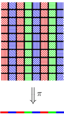
Definition 1. We say that a shift A on Zd is simulated by a shift B on Zd+1
if there exists a projection π : ΣB→ ΣA such that for every configuration
f : Zd+1→ ΣB
from B and for all i1, . . . , id, j, j′ we have π(f(i1, . . . , id, j)) = π(f(i1, . . . , id, j′))
(i.e., the projection π takes a constant value along each column (i1, . . . , id, ∗),
see Fig. 1), and the resulting d-dimensional configuration
{π(f(i1, . . . , id, ∗))}
belongs to A; moreover, each configuration of A can be represented in this way by some configuration of B. Informally, we can say that each configuration from B encodes a configuration from A, and each configuration from A is encoded by some configuration from B.
Theorem 6. (a) Let A be an effective quasiperiodic Zd-shift over some alphabet
ΣA. Then there exists a quasiperiodic SFT B (over another alphabet ΣB) of
dimension d + 1 such that A is simulated by B in the sense of Definition 1. (b) Let A be a Zd-shift simulated in the sense of Definition 1 by some
quasiperiodic SFT B of dimension d + 1. Then A is effective and quasiperi-odic.
=
⇒
π
Figure 1: In this example, each cell of a two-dimensional configuration has two characteristics: the color and the direction of hatching. The color is maintained unchanged along each vertical line. The projection π maps each column to its color.
Remark 2. The parts (a) and (b) of Theorem 6 are the if and only if parts of the following characterization: an effective shift is quasiperiodic if and only if it is simulated by a quasiperiodic SFT of dimension higher by 1.
A similar result holds for effective minimal shifts:
Theorem 7. (a) For every effective minimal Zd-shift A there exists a minimal
SFT B in Zd+1 such that A is simulated by B in the sense of Definition 1.
(b) Let A be a Zd-shift simulated in the sense of Definition 1 by some minimal
SFT B of dimension d + 1. Then A is effective and minimal.
Remark 3. The only if part of this theorem (Theorem 7(b)) is due to the fact that the notion of simulation in Definition 1 is rather restrictive. We should keep in mind that in general a d-dimensional subdynamics of a minimal Zd+1-shift is
not necessarily minimal.
Theorem 6 implies the following rather surprising corollary: a quasiperiodic Z2-SFT can have a highly “complex” language of patterns:
Corollary 1. There exists a quasiperiodic SFT A of dimension 2 such that the Kolmogorov complexity of every (N × N )-pattern in every configuration of A is Ω(N ).
In other words, a quasiperiodic Z2-SFT can have extremely “complex”
lan-guages of patterns.
Remark 4. A standalone pattern of size N × N over an alphabet Σ (with at least two letters) can have Kolmogorov complexity up to Θ(N2). However, this
density of information cannot be enforced by local rules, because in every SFT on Z2 there exists a configuration such that the Kolmogorov complexity of all
N × N -patterns is bounded by O(N ), see [13]. Thus, the lower bound Ω(N ) in Corollary 1 is optimal in the class of all SFT on Z2.
Remark 5. Every effective (effectively closed) minimal shift is computable: given a pattern, we can algorithmically decide whether it belongs to the config-urations of the shift, [15], which is in general not the case for effective quasiperi-odic shift. On the other hand, it is known that patterns of high Kolmogorov complexity cannot be found algorithmically. Thus Corollary 1 cannot be ex-tended to the class of minimal SFT.
1.3
General remarks and organization of this paper
In the theorems stated above, we claim something about (quasiperiodic, min-imal, transitive) SFTs. In the proofs we deal mostly with tilings, which are a very special type of SFT. Since the principal results of the paper are pos-itive statements (we claim that SFTs with some specific properties do exist), the focus on tilings does not restrict the generality. On the other hand, the formalism of Wang tiles perfectly matches the constructions of self-similar and self-simulating shifts of finite type, which are the main technique of this paper. To simplify the notation and make the argument more visual, in what follows we focus on the case d = 2. The proofs extend to any d > 1 in a straightforward way, mutatis mutandis.
The central idea of our arguments is the notion of self-simulation, which goes back to [5] and which was extensively developed in the context of symbolic dynamics in [19]. The technique of hierarchical self-simulating tilings is quite generic and flexible. The drawback of this approach is that it is hard to isolate the core technique from features specific to some particular application. In every specific result we cannot just cite the statement of a previously known theorem about self-simulating tilings: rather, we need to reemploy the constructions from the proofs of a previously known theorem (embedding some new gadgets in the previously known general scheme). This makes the proofs long and somewhat cumbersome. To help the reader, we have tried to make this paper self-contained and explain here the entire machinery of hierarchical self-simulating tilings. The exposition of the main results becomes itself “hierarchical” and “self-similar.” We start with a general perspective of our technique (illustrating it by proofs of several classic results). Then in each succeeding section, we show how to adjust and extend this general construction to obtain this or that new result. We encourage the reader familiar with the concept of self-similar tilings to skip Section 2, which may look oversimplified, and go directly to Sections 3–7.
2
The general framework of self-simulating SFT
In this section we recall the principal ingredients of the technique of self-simulating tile sets. We start this section with a very basic version of a construction of
self-simulating tile sets from [19]. This part of the construction will be enough, in particular, to obtain a proof of the classic Theorem 1. Later, we will extend this construction and adapt it to prove much stronger statements.
2.1
The relation of simulation for tile sets
Let τ be a tile set and N > 1 be an integer. We call a macro-tile an N × N square tiled by matching tiles from τ . Every side of a τ -macro-tile contains a sequence of N colors (of tiles from τ ); we refer to this sequence as a macro-color. Further, let T be some set of τ -macro-tiles (of size N × N ). We say that τ implements T with a zoom factor N if
• some τ -tilings exist, and
• for every τ -tiling there exists a unique lattice of vertical and horizontal lines that cuts this tiling into N × N macro-tiles from T .
A tile set τ simulates another tile set ρ if τ implements a set of macro-tiles T (with a zoom factor N > 1) that is isomorphic to ρ, i.e., there exists a one-to-one correspondence between ρ and T such that the matching pairs of ρ-tiles correspond exactly to the matching pairs of T -macro-tiles. A tile set τ is called self-similar if it simulates itself.
If a tile set τ is self-similar, then all τ -tilings have a hierarchical structure. Indeed, each τ -tiling can be uniquely split into N × N macro-tiles from a set T , and these macro-tiles are isomorphic to the initial tile set τ . Further, the grid of macro-tiles can be uniquely grouped into blocks of size N2× N2, where
each block is a macro-tile of rank 2 (again, the set of all macro-tiles of rank 2 is isomorphic to the initial tile set τ ), etc. It is not hard to deduce that a self-similar tile set τ has only aperiodic tilings (for more details, see [19]). Below, we discuss a generic construction of self-similar tile sets.
2.2
Simulating a tile set defined by a Turing machine
Let us have a tile set ρ. In what follows, we present a general construction that allows to simulate ρ by some other tile set τ , with a large enough zoom factor N . The number of tiles in the simulating tile set τ will be O(N2), and the
constant in the O(·)-notation does not depend on the simulated ρ.
We assume that each color is a string of k bits (i.e., the set of colors C ⊂ {0, 1}k) and the set of tiles ρ ⊂ C4 is presented by a predicate P (c
1, c2, c3, c4)
(the predicate is true if and only if the quadruple (c1, c2, c3, c4) corresponds to
a tile from ρ). Suppose we have a Turing machine M that computes P . (It might look wasteful to construct a Turing machine that computes a predicate with a finite domain, but we will see that this kind of abstraction is useful.) Now we construct in parallel a tile set τ and a set of τ -macro-tiles that simulate the given ρ.
When constructing a tile set τ , we will keep in mind the desired structure of τ -macro-tiles (that should simulate the given tile set ρ). We require that
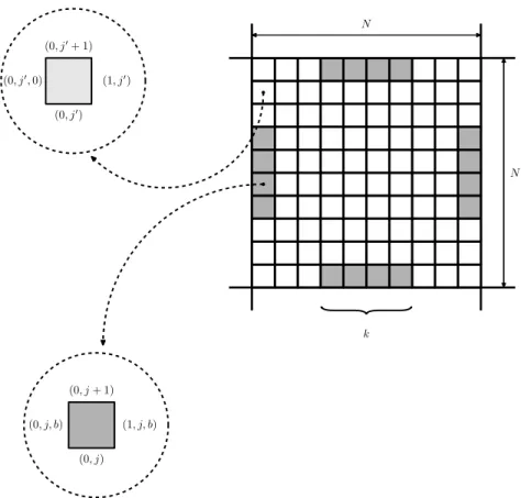
N N (i, j) (i, j + 1) (i, j) (i + 1, j) i j
Figure 2: The basic structure of a macro-tile: A block of size N × N consists of tiles, the coordinates of which in this block (a pair of integers between 0 and N − 1) are written as “colors” of the left and the bottom side of each tile. On the right and on the bottom sides of every tile, one of the coordinates is incremented (modulo N ).
each tile in τ “knows” its coordinates modulo N in the tiling. This information is included in the tile’s colors. More precisely, for a tile that is supposed to have coordinates (i, j) modulo N , the colors on the left and on the bottom sides should involve (i, j), the color on the right side should involve (i + 1 mod N, j), and the color on the top side involve (i, j + 1 mod N ), see Fig. 2.
This means that every τ -tiling can be uniquely split into blocks (macro-tiles) of size N ×N , where the coordinates of the cells range from (0, 0) in the bottom-left corner to (N − 1, N − 1) in top-right corner, as shown in Fig. 2. Intuitively, each tile “knows” its position in the corresponding macro-tile. We will require that in addition to the coordinates, each tile in τ has some supplementary information encoded in the colors on its sides. On the border of a macro-tile (where one of the coordinates of a cell is zero), we assign to the colors of each cell one additional bit of information. Thus, for each macro-tile of size N × N the corresponding macro-colors (in the sense of the definition in Section 2.1, p. 9) can be represented as strings of N zeros and ones.
The number of bits encoding a macro-color (an N -bit string representing a macro-color of a macro-tile of size N × N ) is excessively large for our future constructions. We choose an integer number k (k ≪ N ) and allocate in the middle of a macro-tile’s sides k positions; we make them represent colors from C. The other (N − k) bits on the sides of a macro-tile are “dummy” (formally speaking, we set them all to zero), see Fig. 3.
N N (0, j) (0, j + 1) (0, j, b) (1, j, b) (0, j′) (0, j′+ 1) (0, j′, 0) (1, j′)
{
kFigure 3: We require that tiles on the margins of an N × N macro-tile carry one supplementary bit. For example, the j-th tile on the left margin of a macro-tile contains in the color of its left side a triple (0, j, b), where (0, j) represent the coordinate of this tile in the macro-tile, and the bit b may be equal to 0 or 1. Thus, each macro-color can be now represented by a sequence of N bits embedded in the sides of the tiles on the corresponding margin of a macro-tile. We assume that these supplementary bits are nontrivial only for the k tiles in the middle of each macro-tile’s margin. In the figure, these tiles are shown in gray, e.g., the j-th tile on the left side of a macro-tile carries a bit b, which may be equal to 0 or 1. The other tiles on macro-tile’s margin (e.g., the j′-th
tile on the left side of a macro-tile) do not contribute in the macro-color — their supplementary bits are always set to 0. Thus, each macro-color is actually determined by a sequence of only k bits.
The bits representing the macro-colors are “propagated” in the macro-tile. In what follows we discuss how this information is “processed” inside.
Note that the value of k in our construction is usually much less than N , e.g., k = O(log N ).
that the macro-colors on the macro-tiles satisfy the “simulated” relation P . To this end, we ensure that bits from the macro-tile side are transferred to the central part of the tile, and the central part of a macro-tile is used to simulate a computation of the predicate P . We fix which cells in a macro-tile are “communication wires” and then require that these tiles carry the same (transferred) bit on two sides, see Fig. 4.
The central part of a macro-tile (of size, say, m × m, where m ≪ N ) should represent a space-time diagram of the machine M (the tape is horizontal, and time goes up), see Fig. 5. This Turing machine processes the quadruple of inputs, which are the k-bit strings representing the macro-colors of this macro-tile.
Let us explain in more detail how we represent the computation of a Turing machine in a tiling. First of all, we assume that the machine has a single tape. We understand the space-time diagram of a Turing machine in a pretty standard way, as a table where each vertical column corresponds to one cell on the tape of the machine, and each horizontal row of the diagram represents an instance of a configuration of the Turing machine. For each row of the diagram, we
• specify for each cell (within a bounded part of the tape) the letter written in this position on the tape,
• specify with a special mark the position of the read head, and
• write the index of the internal state of the machine into the cell where the read head is currently located.
Each next row of the diagram represents the configuration of the machine at the next step of computation (once again, we assume that time goes up). Thus, the entire diagram is determined by its bottom line (with the input data of the machine).
The property of being a valid space-time diagram is defined locally, so we can easily represent such diagram of a given Turing machine by local matching rules for tiles. The details of this representation are not very important in the sequel; we may take, for example, the representation described in [7]. In what follows, we need only keep in mind some natural properties of the chosen representation (which trivially hold for the representations from [7]):
• a correct tiling of a frame m × m represents a space-time diagram of the same2size m × m,
• a correct tiling of a frame m × m with some specific bottom line can be formed if and only if the computation (with the corresponding input data) terminates in an accepting state in at most m steps and during this computation the read head never leaves the available finite part of the tape,
2
In fact, it is enough to assume that a tiling of size m × m represents a space-time diagram of size Ω(m) × Ω(m).
(i2, j2) (i2, j2+ 1) (i2, j2,0) (i2+ 1, j2,0) (i2, j2) (i2, j2+ 1) (i2, j2,1) (i2+ 1, j2,1)
or
(i1, j1,0) (i1, j1+ 1) (i1, j1,0) (i1+ 1, j1) (i1, j1,1) (i1, j1+ 1) (i1, j1,1) (i1+ 1, j1)or
{
kFigure 4: In the middle of each margin of a macro-tile we allocate k tiles that contain the bits representing a macro-color. These tiles are plugged into “com-munication wires” that transfer these data inside of a macro-tile. The value of k (which is the width of the red, green, blue, and gray stripes in the figure) is much less than the size of the macro-tile.
In the figure, we zoom in two tiles involved in the “communication wires.” The tile with coordinates (i1, j1) is a part of one of the communication wires
shown in red, which transfer the bits of the top macro-color. As a part of a communication cable, this tile transfers a bit value zero or one. This tile is placed on a corner of a wire, so it “conducts” a bit value from its left side to its bottom side (the bit values embedded in its left and bottom sides must be both zeros or both ones). Similarly, the tile with coordinates (i2, j2) is a part of a
communication wires shown in green, which transfer the bits of the left macro-color. This tile is involved in a horizontal part of a wire, and it “conducts” a bit value zero or one from the left to the right (so the bit values embedded in its left and right sides must be equal to each other).
The coordinates and the values of the transferred bits are embedded in the “colors” on the sides of the tiles. The colors inside individual tiles (red, green, blue, gray in this figure) are only illustrative and show the functional role of each tile in a macro-tile.
Turing machine
Figure 5: A macro-tile with a space-time diagram of a Turing machine in the middle part.
• every (k × k)-fragment3 of a correct tiling can be reconstructed by its
borderline (this is the only property where we need the Turing machine to be deterministic).
The communication of the “computation zone” (the area representing a space-time diagram of a Turing machine) with the “outside world” is restricted to the bottom line (the input data of the computation), which must cohere with the bits representing the four macro-colors of the macro-tile.
To make all of this construction work, the size of a macro-tile (the integer N ) should be large enough: first, we need enough room to place the “communication wires” that transfer the bits of macro-colors to the “computation zone”; second, we need enough time and space in the computation zone of size m × m so that all accepting computations of M terminate in time m and on space m.
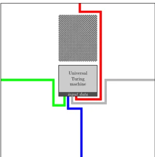
In this construction, the number of additional bits encoded in the colors of the tiles depends on the choice of machine M. To avoid this dependency, we replace M by a fixed universal Turing machine U that runs a program simulating M. Moreover, we prefer to separate the general program of a Turing machine (that involves a description of the predicate P corresponding to the simulated tile set ρ) from the zoom factor N .
Technically, we assume that the tape of the universal Turing machine4 has
an additional read-only layer. Each cell of this layer carries a bit that never changes during the computation (so in the computation zone the columns carry unchanged bits). The construction of a tile set guarantees that these bits form two read-only input fields: (i) the program for M and (ii) the binary expansion of an integer N (which is interpreted as the zoom factor). Accordingly, the computation zone of a macro-tile represents a view of an accepting computation for that program given N as one of the input, see Fig. 6.
3
In what follows we use only a restricted version of this property. We need to be able to reconstruct every (2 × 2)-block of tiles given the 12 tiles around this block, see Fig. 13 below.
4
We assume that the reader is familiar with the basic notions of computability theory. For a detailed discussion of the notion of a universal computable function and universal Turing machines we refer the reader to the textbooks [6, Section II.1] and references therein, and to [10, Section 2.1].
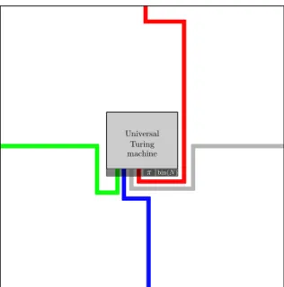
Universal Turing machine
π bin(N )
Figure 6: The computation zone represents a space-time diagram of the univer-sal Turing machine. This machine simulates program π, which gets as input the binary codes of four macro-colors, the binary expansion of the zoom factor N , and its own text.
Thus, from now on we assume that the simulated program is given five inputs: the binary codes of four macro-colors (that are ‘transferred’ from the sides of this macro-tile) and the binary expansion of an integer N (interpreted as the zoom factor).
Without loss of generality, we assume that the positions of the “wires” and the size of the “computation zone” in a macro-tile are chosen in some simple and natural way, and can be effectively computed given the size of the macro-tile N . Moreover, we may assume that the “geometry” of a macro-tile (the positions of the communication wires and of the computation zone) can be computed in polynomial time. That is, given the binary expansions of N, i, j, we can compute in time poly(log N ) the ‘role’ played by a tile with coordinates (i, j) in a macro-tile of size N × N (whether this macro-tile is a part of a wire, or a computation zone, or none of these, and if it belongs to the computation zone, then what bits of the read-only input fields it should carry).
In this way we obtain an explicit construction of a tile set τ that has O(N2)
tiles and simulates ρ. This construction works for all large enough N . Note that most steps of the construction of τ do not depend on the program for M: The tile set τ does depend on the program simulated in the computation zone and on the choice of the zoom factor N . However, this dependency is very limited. The simulated program (and, implicitly, the predicate P ) affects only the rules for the tiles used in the bottom line of the computation zone. The colors on the
sides of all other tiles are generic and do not depend on the simulated tile set ρ. The explicitness of the described construction can be understood quite for-mally as follows: there exists an algorithm that takes the binary expansions of N , k, m and a program for M as an input, and returns the list of tiles in the tile set τ described above. The algorithm halts with an appropriate warning if N , k, or m is too small for our construction. Moreover, for every quadruple of colors we can verify in polynomial time (in time poly(log N )) whether this quadruple forms a tile in τ or not.
2.3
Self-simulation with Kleene’s recursion technique
In the previous section we explained how to simulate any given tile set ρ by another tile set τ with a large enough zoom factor N . Now we want to find a ρ such that the corresponding simulating tile set τ is isomorphic to the simulated ρ. We achieve this by using an idea that comes from the proof of Kleene’s recursion theorem. Roughly speaking, we employ the idea that a program can somehow access its own text and use its bits in the computation. In most textbooks, the proof of Kleene’s recursion theorems involves the so-called s-m-n theorem, which explains how an algorithm can process the source codes of other programs (given as an input), see e.g. [6]. For a more informal discussion of the ideas behind Kleene’s recursion theorems we recommend [10].
Our goal is to construct a tile set τ that simulates itself. At the end of the previous section we observed that our construction of a simulating tile set τ has a very limited dependency on M (and, therefore, on the simulated tile set ρ). Let us fix a triple of parameters k, m, N ; we apply the construction from the previous section and produce the list of all tiles from the tile set τ that simulates some tile set ρ (the simulated tiles may use at most 2k colors; N is the zoom
factor and m is the size of the computation zone in τ -macro-tiles). Since the simulated ρ is not fixed yet, we cannot produce the complete list of tiles in τ ; we obtain only those tiles that do not depend on the simulated tile set, i.e., all tiles except for the tiles that appear in the bottom line of the computation zone. In what follows we choose the missing tiles in such a way that the resulting τ simulates itself.
To complete the construction, we will add to τ a few other tiles (exactly those tiles that appear in the bottom line of the computation zone). This construction will work for k = 2 log N + O(1) (so that we can encode O(N2) colors in strings
of k bits) and m = poly(log N ) (so that we can put in the computation zone a space-time diagram of a polynomial-time computation of the Universal Turing machine).
Though the definition of τ is not finished, we already know that every valid τ -tiling (if such a tiling exists) consists of an N × N -grid of macro-tiles, with k-bit macro-colors embedded in their sides, with communication wires and a computation zone, as shown in Fig. 6. We want to construct a program π that takes as an input the integers k, m, N , and four k-bit strings embodying macro-colors, and checks that a macro-tile with the given macro-colors represents one of the tiles in the would-be τ . Then we embed this program in the tile set τ
and complete the construction.
Now let us focus on the program π that should perform the necessary checks (these checks should be simulated in the computation zone of every macro-tile). For the macro-tiles that represent the tiles that are already included in τ , the required checks are straightforward (see the comment at the end of the previous section). It remains to implement (and encode in the program π) the checks for the tiles of τ that are not defined yet.
Let us remind that the tiles in τ that are still missing are exactly the tiles that should represent the hardwired program. This might seem as a paradox: we have to write a text of a program that handles the tiles where this program will be hardwired. On the one hand, we need to know these tiles to write a program; on the other hand, we need to know the text of the program to produce the tiles. However, we can complete the description of the program π without knowing the missing tiles of τ . Since in our construction of a macro-tile, the would-be program π (the list of instructions interpreted by the universal Turing machine) is written on the tape of the universal machine, this program can be instructed to access the bits of its own “text” and check that if a macro-tile plays a role of a tile in the computation zone, then this macro-tile carries the correct bit of the program.
This is the crucial point of the construction. The algorithm implemented in π can be explained as follows. The algorithm obtains as an input the bits encoding the four colors of the tile. We suppose that a macro-tile represents a macro-tile from τ , and we know that each τ -macro-tile contains a pair of coordinate (i, j) modulo N . We can extract these coordinates (i, j) from the macro-colors of the macro-tile. If this position does not belong to the bottom line of the computation zone of a macro-tile, then our task is simple: we use the algorithm outlines at the end of the previous section. But if the position (i, j) corresponds to the bottom line in the computational zone, then the task is subtle: in this case the τ -tile represented by this macro-tile must involve some bit from the text of π (and it should be encoded in the color on the top side of the macro-tile). How to check that the corresponding bit embedded in the macro-color is correct? Where do we get the “correct” value of this bit? The answer is straightforward: the Universal Turing machine simulating π should move its reading head to the column j in its own computation zone and read there the required bit value. Note that there is no chicken-and-egg paradox, we can write the instructions for π before we know its full text.
Thus, we obtain the complete text (list of instructions) of the program π. This is exactly the program that should be simulated by the Universal Turing machine in the computational zone of each macro-tile, so it is the program whose text must be written on the bottom line of the computation zone. This program provides us with the missing part of the tile set τ (we supplement the tile set τ with the tiles that represent in the bottom line of the computation zone the text of π).
It remains to choose the parameters N and m. We need them to be large enough so that the computation described above (which deals with inputs of size O(log N )) can fit in the computation zone. The computations are rather simple
(polynomial in the input size, i.e., polynomial in O(log N )), so they fit in the space and time bounded by m = poly(log N ). Thus, we set m(N ) = poly(log N ) for some specific polynomial that is not too small (e.g., m := (log N )3is enough)
and choose N large enough so that m(N ) ≪ N , and the geometry of a macro-tile shown on Fig. 6 can be realized. This completes the construction of a self-similar aperiodic tile set. Now, it is not hard to verify that the constructed tile set (i) allows a tiling of the plane, and (ii) is self-similar.
The construction described above works well for all large enough zoom fac-tors N . In other words, for all large enough N we get a self-similar tile set τN,
and the tilings for all these τN have very similar structure, with macro-tiles as
shown in Fig. 6. Technically, the program π (simulated by the universal Turing machine) now takes as its input a tuple of six strings of bits: the bit strings of length k = k(N ) representing the four macro-colors of a macro-tile, the binary expansion of the zoom factor N , and its own text. This program checks whether the given strings are coherent, i.e., whether the given quadruple of macro-colors in fact represents a quadruple of colors of one tile in our self-similar tile set τN
(corresponding to the given value N of the zoom factor).
The presented construction of a self-simulating tile set provides a proof of Theorem 1, see a comment at the end of Section 2.1. Indeed, if a tile set τ simulates itself with a zoom factor N , then by definition every τ tiling can be uniquely split into N × N macro-tiles. Since these macro-tiles are isomorphic to the tiles of τ , the grid of macro-tiles can be uniquely split into macro-macro-tiles of size N2× N2. The macro-macro-tiles are obviously also isomorphic to the
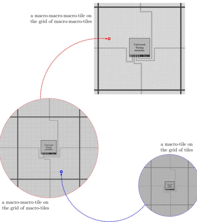
τ -tiles, so they also can be batched in macro-tiles of higher rank, and so on. We obtain a hierarchical structure of macro-tiles of rank k = 1, 2, . . ., see Fig. 7.
For discussion of the technique of self-simulating tilings and a motivation behind it we refer the reader to [19]. In what follows, we extend and gener-alize this construction step by step, and then apply it to prove much stronger statements.
Notation. We now introduce some useful terminology. In a hierarchical structure of macro-tiles, if a level-k macro-tile M is a cell in a level-(k + 1) macro-tile M′, we refer to M′ as the father of M . We refer to the level-(k + 1)
macro-tiles neighboring M′ as the uncles of M .
2.4
A more flexible construction: The choice of the zoom
factor
For a large class of sufficiently “well-behaved” sequences of integers Nk, we can
construct a family of tile sets τk (i = 0, 1, . . .) such that each τk−1 simulates
the next τk with the zoom factor Nk (and, therefore, τ0simulates each τk with
zoom factor Lk = N1· N2· · · Nk).
The idea is to reuse the basic construction from the previous section and vary the sizes of the macro-tiles (the zoom factors) on the different levels of the hierarchy. While in the basic construction the macro-tiles (built of N × N tiles), the macro-macro-tiles (built of N ×N macro-tiles), the macro-macro-macro-tiles
Universal Turing machine πbin(N ) Universal Turing machine πbin(N ) Universal Turing machine πbin(N ) a macro-tile on the grid of tiles
a macro-macro-tile on the grid of macro-tiles
a macro-macro-macro-tile on the grid of macro-macro-tiles
Figure 7: Hierarchical structure of macro-tiles. The level-k macro-tiles are blocks in the level-(k + 1) macro-tiles, the level-(k + 1) macro-tiles are blocks in level-(k + 2) macro-tiles, etc. On all levels of the hierarchy, the structure of the macro-tiles is pretty much the same.
(built of N × N macro-macro-tiles), and so on, behave in exactly the same way, in the revised construction the behavior of a level-k macro-tile depends on k. We want to have macro-tiles built of N1× N1 ground-level tiles,
macro-macro-tiles built of N2× N2 macro-tiles, macro-macro-macro-tiles built of N3× N3
macro-macro-tiles, and so on. In this construction, the level-k macro-tiles will be isomorphic to the tiles of τk, and the idea of “self-simulation” should be
understood less literally.
To implement this idea, we need only a minor revision of the construction from the previous section. Similar to our basic self-simulation construction, each tile of τk “knows” its coordinates modulo Nk in the tiling: the colors on
the left and on the bottom sides should involve (i, j), the color on the right side should involve (i + 1 mod Nk, j), and the color on the top side involves
(i, j+1 mod Nk). Consequently, every τk-tiling can be uniquely split into blocks
(macro-tiles) of size Nk×Nk, where the coordinates of the cells range from (0, 0)
in the bottom-left corner to (Nk− 1, Nk− 1) in the top-right corner, similarly to
Fig. 2. Again, intuitively, each macro-tile of level k “knows” its position in the corresponding macro-tile of level (k + 1). For each k, the Nk× Nk-macro-tile
(built of tiles τk) should have the structure shown in Fig. 6, with communication
wires, a computation zone, and auto-referential computation inside.
The difference with the basic construction is that now the computation sim-ulated by a level-k macro-tile gets, as an additional input, the value k, and the zoom factor Nk is computed as a function of k. In what follows, we always
assume that Nk can be easily computed given the binary expansion of k (say,
in time poly(log Nk)).
Technically, we assume now that the first line of the computation zone con-tains the following fields of the input data:
(i) the program of a Turing machine π that verifies whether a quadruple of macro-colors corresponds to a valid macro-color,
(ii) the binary expansion of the integer rank k of this macro-tile (the level in the hierarchy of macro-tiles),
(iii) the bits encoding the macro-colors: each macro-color involves the position inside the father macro-tile of rank (k + 1) (two coordinates modulo Nk+1)
and O(1) bits of the supplementary information assigned to the macro-colors.
Note that now the zoom factor is not provided explicitly as one of the input fields. Instead, we have the binary expansion of k, so that a Turing machine can compute the value of Nk, see Fig. 8. The difference from Fig. 6 is that the
computation in the macro-tile of rank k gets as an input the index k instead of the universal zoom factor N .
As before, we require that the simulated computation terminates in an ac-cepting state if the macro-colors of the macro-tile form a valid quadruple (if not, no correct tiling can be formed). The simulated computation guarantees that the macro-tiles of level k are isomorphic to the tiles of τk+1.
Universal Turing machine
π bin(k)
Figure 8: A macro-tile of level k. The computation zone represents the universal Turing machine that simulates a program π, which gets as input the binary codes of four macro-colors, the binary expansion of the level k, and the text of π itself.
Note that on each level k of the hierarchy, we simulate in macro-tiles a computation of one and the same Turing machine π. Only the inputs for this machine (including the binary expansion of the rank k) vary from level to level. This construction works well if Nk does not grow too slowly (so that the
level-k macro-tiles have enough room to keep the binary expansion of k) yet not too fast (so that the computation zone in the level-k macro-tiles can handle elementary arithmetic operations with Nk+1). In what follows we assume that
Nk= 3C
k
for some large enough constant C.
The growing zoom factor Nk allows embedding some payload in the
com-putation zone: some “useful” comcom-putation that has nothing to do with self-simulation but affects the properties of a tiling. More precisely, we require that the program π (whose simulation by the Universal Turing machine is em-bedded in each macro-tile) performs two different tasks: its primary job is to perform the checks of consistency for the four macro-colors of the correspond-ing macro-tile, as explained above; the secondary job is to run some specific “useful” algorithm A. In each proof based on this technique we use a particular algorithm A (which is explicitly hardwired in the program π and, therefore, implicitly embedded in the constructed tile set). If necessarily, this algorithm may access as an input the macro-colors of the corresponding macro-tile (they are available in the computation zone). A priori, the computation of A can be infinitely long. We assume that in each macro-tile the simulation of A is performed within the limits of the allocated space and time (the size of the
“computation zone”), and the simulation is aborted when the Universal Turing machine runs out these limits. Though all macro-tiles (on all levels of the hier-archical structure) simulate one and the same algorithm A, the available space depends on the rank of a macro-tiles. Since the zoom factor grows with the rank, on each subsequent level of the hierarchy of macro-tiles we can allocate to this secondary computation more and more space and time.
Remark 6. The presented construction of a self-simulating tile set is enough to prove the existence of an SFT where each configuration is non-computable (the result known from [3, 4]), for details, see [19].
3
Quasiperiodic self-simulating SFT
In this section, we revise once again the construction of a self-simulating tiling and enforce the property of quasi-periodicity or minimality. In particular, this construction will give a new proof of Theorem 2. To implement this construc-tion, we have to superimpose some new properties of a self-simulating tiling.
3.1
Supplementary features: Constraints that can be
im-posed on the self-simulating tiling
The tiles involved in our self-simulating tile set (as well as all macro-tiles of each rank) can be classified into three types:
(a) the “skeleton” tiles, which keep no information except for their coordinates in the father macro-tile (the white area in Fig. 8; each of these tiles looks like the tile shown in Fig. 2): these tiles work as building blocks of the hierarchical structure;
(b) the “communication wires,” which transmit the bits of the macro-colors from the borderline of the macro-tile to the computation zone (the colored lines in Fig. 8; each of these tiles looks like the tiles shown in Fig. 4); (c) the tiles of the computation zone (intended to simulate the space-time
diagram of the Universal Turing machine, the gray area in Fig. 8). Each pattern that includes only “skeleton” tiles (or “skeleton” macro-tiles of some rank k) reappears infinitely often in all homologous positions inside all macro-tiles of higher rank. Unfortunately, this property is not true for the pat-terns that involve the “communication zone” or the “communication wires.” Thus, the basic construction of a self-simulating tiling does not imply the prop-erty of quasiperiodicity. To overcome this obstacle we need several new technical tricks.
First of all, we impose several restrictions on our construction of a self-simulating tiling. These restrictions in themselves do not make the tilings quasiperiodic, but they simplify the upcoming revision of the construction. More specifically, we enforce the following additional properties (p1)–(p4) of a tiling, with only a minor modification of the construction.
Universal Turing machine
input data
Figure 9: The “free” area reserved above the computation zone.
(p1) In our basic construction, each macro-tile contains a computation zone of size mk, which is much less than the size of the macro-tile Nk. In what follows,
we need to reserve free space in a macro-tile, in order to insert O(1) (some constant number) of copies of each (2 × 2)-pattern from the computation zone (of this macro-tile), right above the computation zone. This requirement is easy to meet. We assume that the size of a level-k macro-tile (measured in blocks that are themselves macro-tiles of level k − 1) is Nk× Nk, and the computation
zone in this macro-tile is mk× mk for mk = poly(log Nk). Therefore, we can
reserve an area of size Θ(mk) right above the computation zone, which is free
of “communication wires” or any other functional gadgets, see the “empty” hatched area in Fig. 9. So far, this area consisted of only skeleton tiles; in what follows (Section 3.2 below), we will use this zone to place some new nontrivial elements of the construction.
(p2) We require that the tiling inside the computation zone satisfies the prop-erty of 2 × 2-determinacy. That is, if we know all of the colors on the borderline of a 2 × 2-pattern inside the computation zone (i.e., a tuple of 8 colors), then we can reconstruct the four tiles of this pattern. Again, we do not need any new ideas to implement this property. It is not hard to see that this requirement is met if we represent the space-time diagram of a Turing machine in a natural way (see the discussion on p. 14).
(p3) The communication channels in a macro-tile (the wires that transmit infor-mation from the macro-color on the borderline of this macro-tile to the bottom line of its computation zone) must be isolated from each other. The gap
be-Universal Turing machine
input data
Figure 10: The wires in the “communication cables” (shown in red, blue, green, and gray in the figure) are separated by a gap (shown in white), so that the distance (measured in tiles) between every two wires is greater than two.
tween every two wires must be greater than two cells, as shown in Fig. 10. In other words, each group of cells of size 2 × 2 can touch at most one communi-cation wire. Since the number of wires in a level-k macro-tile is only O(log Nk),
we have enough free space to lay the “communication cables” maintaining the required safety gap, so this constraint is easy to satisfy.
(p4) In our construction, the macro-colors of a level-k macro-tile are encoded by bit strings of length rk = O(log Nk+1). In the previous section we only
assumed that this encoding is somewhat “natural” and easy to handle. So far, the choice of encoding was of small importance: we only required that some natural manipulations with macro-colors could be implemented in polynomial time.
We now add another (seemingly artificial) condition. We have decided that each macro-color is encoded in a string of rk bits. We require now that each
bit in this encoding takes both values 0 and 1 quite often. More precisely, we require that for each i = 1, . . . , rk there are quite many macro-tiles where the
ith bit of encoding of the top (bottom, left, right) macro-color is equal to 0, and there are quite many other macro-tiles where the ith bit of this encoding is equal to 1. In what follows we specify what the words quite often and quite many mean in this context.
Technically, we use the following property: for every position s = 1, . . . , rk
• there exists j0such that the sth bit in the top, left, and right macro-colors
of the level-k macro-tile at the positions (i, j0) in the level-(k + 1) father
macro-tile are equal to 0, and
• there exists j1such that the sth bit in the top, left, and right macro-colors
of the level-k macro-tile at the positions (i, j1) in the level-(k + 1) father
macro-tile are equal to 1.
There are many (more or less artificial) ways to implement this constraint. For example, we may subdivide the array of rkbits encoding a macro-color into three
equal zones of size rk/3 and require that for each macro-tile only one of these
three zones contains the “meaningful” bits, and the two other zones contain only zeros and ones respectively; we require then that the “roles” of these three zones cyclically permute as we go upwards along a column of macro-tiles, see Fig. 11.
3.2
Enforcing minimality
To achieve the property of minimality of an SFT, we should guarantee that every finite pattern that appears once in at least one tiling must also appear in every large enough square in every tiling. In a tiling with a hierarchical structure of macro-tiles each finite pattern can be covered by at most four macro-tiles (by a 2 × 2-pattern) of an appropriate rank. Hence, to guarantee the property of minimality, it is enough to show that every (2 × 2)-block of macro-tiles of any rank k that appears in at least one τ -tiling actually reappears in this tiling in every large enough square. Let us classify all (2 × 2)-block of macro-tiles (by their position in the father macro-tiles of higher rank) and discuss what revisions of the construction are needed.
Case 1: Skeleton tiles. For a (2 × 2)-block of four “skeleton” macro-tiles of level k, there is nothing to do. Indeed, in our construction we have exactly the same blocks with every vertical translation by a multiple of Lk+1 (we have
there a similar block of level-k “skeleton” macro-tiles contained in some other macro-tile of rank (k + 1)).
Case 2: Communication wires. Let us consider the case when a (2 × 2)-block of level-k macro-tiles involves a part of a communication wire. Due to property (p3) we may assume that only one wire is involved. The bit transmitted by this wire is either 0 or 1; in either case, due to property (p4), we can find another similar (2×2)-block of level-k macro-tiles (at the same position within the father macro-tile of rank (k + 1) and with the same bit included in the communication wire) in every macro-tile of level (k + 2). In this case we can find a duplicate of the given block with a vertical translation of size O(Lk+2).
Case 3: Computation zone. Now we consider the most difficult case: when a (2 × 2)-block of level-k macro-tiles touches the computation zone. In this case we cannot obtain the property of quasiperiodicity for free, and so we have to make one more modification to our general construction of a self-simulating tiling.
Universal Turing machine πbin(N ) Universal Turing machine πbin(N ) Universal Turing machine πbin(N ) Universal Turing machine πbin(N ) macro-colors encoded as 000 . . . 0 | {z } rk/3 111 . . . 1 | {z } rk/3 [nontrivial part] | {z } rk/3 macro-colors encoded as 111 . . . 1 | {z } rk/3 [nontrivial part] | {z } rk/3 000 . . . 0 | {z } rk/3
macro-colors encoded as [nontrivial part]
| {z } rk/3 000 . . . 0 | {z } rk/3 111 . . . 1 | {z } rk/3 macro-colors encoded as 000 . . . 0 | {z } rk/3 111 . . . 1 | {z } rk/3 [nontrivial part] | {z } rk/3
Figure 11: Encoding of macro-colors. The rkbits of the code are split into three
blocks of size rk/3. One of them consists of all 0s, another of all 1s, and only
the third one contains a nontrivial binary code. The roles of the three blocks change cyclically from one macro-tile to another when we move upwards.
Universal Turing machine
input data
Figure 12: Positions of the diversification slots for patterns from the computa-tion zone.
Note that for each 2 × 2-window that touches the computation zone of a macro-tile, there are only O(1) ways to tile them correctly. For each possible position of a 2 × 2-window in the computation zone and for each possible filling of this window by tiles, we reserve a special 2 × 2-slot in a macro-tile, which is essentially a block of size 2 × 2 in the “free” zone of a macro-tile. We refer to this gadget as a diversification slot. These slots will enforce the property of “diversity”: for every small pattern that could appear in the computation zone, we will guarantee that it must appear in the corresponding diversity slot in every macro-tile of the same rank.
The diversification slots must be placed far away from the computation zone and from all communication wires. We prefer to place every diversification slot in the same vertical stripe as the “original” position of this block, as shown in Fig. 12 (this property of vertical alignment will be used in Section 6). We have enough free space to place all necessary diversification slots, due to property (p1). We define the neighbors around each diversification slot in such a way that only one specific (2 × 2)-pattern can patch it (here we use the property (p2)).
In our construction, the tiles around this slot “know” their real coordinates in the bigger macro-tile, while the tiles inside the diversification slot do not (they “believe” they are tiles in the computation zone, while in fact they belong to an artificial isolated “diversity preserving” slot far outside of any real computation), see Fig. 12 and Fig. 13. The frame of the diversification slot consists of 12
(i, j) (i, j + 1) (i, j) (i, j + 1) (i + 1, j) (s, t) (i + 1, j) (i + 2, j) (i + 2, j) (s + 1, t) (i + 2, j) (i + 3, j) (i + 3, j) (i + 3, j + 1) (i + 3, j) (i + 4, j) (i, j + 1) (i, j + 2) (i, j + 1) (s, t) (s, t) (s, t + 1) (s, t) (s + 1, t) (s + 1, t) (s + 1, t + 1) (s + 1, t) (s + 2, t) (i + 3, j + 1) (i + 3, j + 2) (s + 2, t) (i + 4, j + 1) (i, j + 2) (i, j + 3) (i, j + 2) (s, t + 1) (s, t + 1) (s, t + 2) (s, t + 1) (s + 1, t + 1) (s + 1, t + 1) (s + 1, t + 2) (s + 1, t + 1) (s + 2, t + 1) (i + 3, j + 2) (i + 3, j + 3) (s + 2, t + 1) (i + 4, j + 2) (i, j + 3) (i, j + 4) (i, j + 3) (i + 1, j + 3) (s, t + 2) (i + 1, j + 4) (i + 1, j + 3) (i + 2, j + 3) (s + 1, t + 2) (i + 2, j + 4) (i + 2, j + 3) (i + 3, j + 3) (i + 3, j + 3) (i + 3, j + 4) (i + 3, j + 3) (i + 4, j + 3)
Figure 13: A diversification slot for a 2 × 2-pattern from the computation zone.
“skeleton” tiles (the white squares in Fig. 13); they form a slot that involves inside a (2 × 2)-pattern extracted from the computation zone (the gray squares in Fig. 13). In the picture, we show the “coordinates” encoded in the colors on the sides of each tile. Note that the colors of the bold lines (the blue lines between the white and gray tiles and the bold black lines between the gray tiles) should contain some information beyond the coordinates—these colors involve the bits used to simulate a space-time diagram of the universal Turing machine. In this picture, the “real” coordinates of the bottom-left corner of this slot are (i + 1, j + 1), while the “natural” coordinates of the pattern inside the diversification slot (when this pattern appears in the computation zone) are (s, t).
We choose the positions of the diversification slots in the macro-tile so that the coordinates can be computed by some simple algorithm in time polynomial in log Nk. We require that all diversification slots be detached from each other
in space, so they do not damage the general structure of the “skeleton” tiles building the macro-tiles.
Now it is not hard to see that for the revised tile set, every pattern that ap-pears at least once in at least one tiling must in fact appear in every large enough pattern in every tiling. Thus, the revised construction of a self-simulating tiling guarantees that
• every tiling is aperiodic (the argument from the previous section remains valid), and
• every pattern that appears at least once in at least one configuration must appear in every large enough square in every tiling.
Hence, our construction implies Theorem 2.
4
Quasiperiodicity and non-computability
So far, we have used the method of self-simulating tilings to combine the prop-erties of quasiperiodicity (and even minimality) and aperiodicity. Now we are going to go further and combine quasiperiodicity with non-computability. In this section, we extend the construction discussed above and prove Theorem 3 and Theorem 4. To this end, we extensively use the technique of a self-simulating tiling with a variable zoom factor, introduced in Section 2.4. As we mentioned above, we assume that the size of a macro-tile of rank k is equal to Nk× Nk,
for Nk = 3C
k
, k = 1, 2, . . ., and the size of the computation zone mk grows as
mk= poly(log Nk).
We take as the starting point the generic scheme of a quasi-periodic self-simulating tiling explained in the previous section, and adjust it with some new features. From now on we require that all macro-tiles of rank k contain, in their computation zone, the prefix (e.g., of length ⌈log k⌉) of some infinite sequence X = x0x1x2. . . We want that all macro-tiles of rank k contain the same prefix
x0x1x2. . . k⌈log k⌉, so we will embed these bits in the colors of all
macro-tiles. To make things more pictorial, we require also that these bits be provided in the bottom line of the computation zone as one supplementary input field, as shown in Fig. 14. But we stress again that the bits x0x1x2. . . k⌈log k⌉make part
of each macro-color. So in Fig. 14 these bits are repeated five times: they appear four times implicitly as a part the codes of macro-colors (greed, blue, gray, and red fields in the picture) and one more time explicitly (the rightmost part of the computation zone). The computation hidden in each macro-tile should verify that these five copies of x0x1x2. . . k⌈log k⌉provided to the computation zone are
identical.
Since every two neighboring macro-tiles must have matching macro-colors, we can guarantee every two neighboring level-k macro-tiles contain one and the same prefix x0x1x2. . . k⌈log k⌉ (this remains true even for neighboring level-k
macro-tiles that belong to different father macro-tiles of level (k + 1)). Thus, the construction implies that in each valid configuration all level-k macro-tiles involve one and the same prefix x0x1x2. . . k⌈log k⌉.
We also need coherence between bits xiembedded in macro-tiles of different
ranks (the string embedded in a macro-tile of higher rank should extend the string embedded in macro-tiles of lower rank). So we suppose that the compu-tation embedded in the compucompu-tational zones of macro-tiles verifies whether the input data are coherent, i.e., that the bits embedded in each of the four macro-tiles match the bits x0x1x2. . . k⌈log k⌉ given explicitly in this new input field.
Using the usual self-simulation, we can guarantee that the bits of X embedded in a macro-tile of rank k + 1 extend the prefix embedded in a macro-tile of rank k. Since the size of the computation zone increases as a function of k, the entire tiling of the plane determines an infinite sequence of bits X (whose prefixes are encoded in the macro-tiles of all ranks).
time-space diagram of
the Universal Turing
machine
program π bin(k) x0x1. . . xlog k
. . . .
Figure 14: The computation zone of a macro-tile in the revised construction. The input data consist of the codes of the macro-colors, the simulated program π, the binary expansion of the rank k, and the first log k bits of the embedded sequence X = x0x1x2. . .
Remark 7. The new feature allows embedding an infinite sequence X in a tiling. This embedding is highly distributed in the following sense: we can extract the first log k bits of the sequence from any level-k macro-tile. Note that the tile set does not determine the embedded sequence X (different tilings of the same tile set can represent different sequences X). However we are going to control the class of sequences X that can be embedded in a tiling.
Since the embedded sequence X is not uniquely defined by the tile set, we lose the property of minimality (different τ -tilings involve different embedded sequences X, and therefore different finite patterns). However, we still have the property of quasiperiodicity. Indeed, every valid tiling contains a well-defined embedded sequence X. Let us fix one infinite sequence X and restrict ourselves to the class of tilings T (X) that represent this specific sequence. Then, all level-k macro-tiles in every tiling in T (X) involve (one and the same) prefix of X. Now the argument from the previous section, repeated word for word, gives the following property.
Every (2 × 2)-block of level-k macro-tiles that appears at least once in at least one tiling in T (X) must reappear in every large enough pattern of every tiling in T (X).
It follows immediately that every tiling in this construction is quasiperiodic. When the class of embedded sequences of X is not restricted, this construc-tion is of no interest. It becomes meaningful if we can enforce some special properties of the embedded sequence X.