HAL Id: hal-00296279
https://hal.archives-ouvertes.fr/hal-00296279
Submitted on 6 Jul 2007
HAL is a multi-disciplinary open access
archive for the deposit and dissemination of
sci-entific research documents, whether they are
pub-lished or not. The documents may come from
teaching and research institutions in France or
abroad, or from public or private research centers.
L’archive ouverte pluridisciplinaire HAL, est
destinée au dépôt et à la diffusion de documents
scientifiques de niveau recherche, publiés ou non,
émanant des établissements d’enseignement et de
recherche français ou étrangers, des laboratoires
publics ou privés.
sounding of the atmosphere
R. Sussmann, T. Borsdorff
To cite this version:
R. Sussmann, T. Borsdorff. Technical Note: Interference errors in infrared remote sounding of the
atmosphere. Atmospheric Chemistry and Physics, European Geosciences Union, 2007, 7 (13),
pp.3537-3557. �hal-00296279�
www.atmos-chem-phys.net/7/3537/2007/ © Author(s) 2007. This work is licensed under a Creative Commons License.
Chemistry
and Physics
Technical Note: Interference errors in infrared remote sounding of
the atmosphere
R. Sussmann and T. Borsdorff
IMK-IFU, Forschungszentrum Karlsruhe, Kreuzeckbahnstrasse 19, 82467 Garmisch-Partenkirchen, Germany Received: 13 November 2006 – Published in Atmos. Chem. Phys. Discuss.: 12 December 2006
Revised: 26 March 2007 – Accepted: 31 May 2007 – Published: 6 July 2007
Abstract. Classical error analysis in remote sounding
distin-guishes between four classes: “smoothing errors,” “model parameter errors,” “forward model errors,” and “retrieval noise errors”. For infrared sounding “interference errors”, which, in general, cannot be described by these four terms, can be significant. Interference errors originate from spectral residuals due to “interfering species” whose spectral features overlap with the signatures of the target species. A general method for quantification of interference errors is presented, which covers all possible algorithmic implementations, i.e., fine-grid retrievals of the interfering species or coarse-grid retrievals, and cases where the interfering species are not re-trieved. In classical retrieval setups interference errors can exceed smoothing errors and can vary by orders of magnitude due to state dependency. An optimum strategy is suggested which practically eliminates interference errors by systemat-ically minimizing the regularization strength applied to joint profile retrieval of the interfering species. This leads to an interfering-species selective deweighting of the retrieval. De-tails of microwindow selection are no longer critical for this optimum retrieval and widened microwindows even lead to reduced overall (smoothing and interference) errors. Since computational power will increase, more and more opera-tional algorithms will be able to utilize this optimum strat-egy in the future. The findings of this paper can be ap-plied to soundings of all infrared-active atmospheric species, which include more than two dozen different gases relevant to climate and ozone. This holds for all kinds of infrared remote sounding systems, i.e., retrievals from ground-based, balloon-borne, airborne, or satellite spectroradiometers.
1 Introduction
During the last decade, more and more, infrared remote sounding measurements have been used to obtain profiles
Correspondence to: R. Sussmann
of atmospheric composition and temperature from ground or space. Infrared profiling techniques complement the older microwave profilers in many ways, e.g., with respect to the altitude range attainable and the atmospheric trace species under consideration. The theoretical framework for the retrieval of profiles from spectral measurements via opti-mal estimation was developed three decades ago (Rodgers, 1976) and was applied to microwave soundings in the begin-ning. Later, a concept for the error analysis was formulated (Rodgers, 1990, 2000; Connor et al., 1995) to distinguish between four different classes of errors, i.e., “smoothing er-rors”, “model parameter erer-rors”, “forward model erer-rors”, and “retrieval noise errors”. This classical error analysis has also been applied to infrared retrievals. However, in the infrared, a very frequently encountered problem in retrieving the “tar-get quantity” is due to “interfering species”. This occurs be-cause the vibration-rotation bands of different species often overlap in the infrared atmospheric spectrum. Keeping in mind that the wings of (infrared) spectral lines always expand asymptotically towards plus-minus infinity in the frequency domain, it becomes clear that individual spectral lines used for the profile retrieval of an atmospheric target species, in principle, always overlap with neighboring spectral lines of other interfering species. This leads to “interference errors” that can, in general, not be treated by either of the above mentioned four terms of classical error analysis.
Throughout this paper the term “interference error” refers to all errors that originate from any type of soft or hard con-straint imposed on the retrieval of the profile of an interfering species in an algorithm; this causes spectral residuals (mea-sured minus simulated) around the spectral signature of the interfering species. In consequence, the profile retrieval of the target species tends to compensate for this, meaning that an artifact is introduced into the retrieved target profile.
In addition to the described effect from interfering species we will also include in the term “interference error” all errors from constraints imposed on the retrieval of any additional,
varying, vector-type physical quantity which impacts the measurement vector. One example are temperature profiles, which are retrieved jointly with the target species in some retrieval setups in order to minimize errors from insufficient knowledge of the true temperature profile at the time of ob-servation. For simplicity, we will hereafter extend the term “interfering species” to include these additional interfering vectors.
It is also important to specify, what our concept of inter-ference errors does not mean throughout this paper. It does not have to do with any intrinsic error in the forward mod-eling, i.e., either with errors in the forward model param-eters, such as errors in the spectroscopic parameters of in-terfering species, or with errors in the forward model itself like errors in line shape modeling. Both kinds of errors also lead to residuals in the retrieval of the interfering species and thereby introduce errors to the retrieval of the target species, and, therefore, might also be entitled “interference errors”. However, these two error classes can be clearly attributed to and treated as “model parameter errors” (above example of errors in spectroscopic parameters) and to “forward model errors” (above example of errors in line shape modeling), and we will not further treat them within this paper.
This being said we like to point to an exception, i.e., a spe-cial case where interference errors in the sense of our paper can in fact be treated by the existing concept of “model pa-rameter errors” as defined in Rodgers (2000, Eq. 3.16, second term): interfering species are sometimes not retrieved due to computation power limitations, e.g., in satellite infrared re-mote sensing. Interference errors originate in this case from a different effect. They do not arise from any constraint to the retrieval of interfering species (because they are not re-trieved), nor from intrinsic forward model or model param-eter errors, but from neglecting the likely discrepancies be-tween the true profile of an interfering species at the moment of observation and its fixed a priori profile used for forward modeling. This again leads to spectral residuals that intro-duce errors to the retrieval of the target species. Formally, the discrepancies between the true profile of an interfering species and the one used for forward modeling can be treated by the concept of model parameter errors. This kind of error quantification for the case of unretrieved interfering species has been performed previously, and a minimization of inter-ference errors in this case was achieved by optimized mi-crowindow selection, i.e., an extensive mimi-crowindow cutting aiming at a minimized inclusion of spectral signatures of in-terfering species while preserving the main features of the target species (e.g., von Clarmann and Echle, 1998; Echle et al., 2000; Dudhia et al., 2002).
An alternative approach is to jointly retrieve the interfering species and the target species at the same time. This leads to a reduced interference effect compared to the case of unre-trieved interfering species for a given microwindow set. This is achieved at the cost of increased computation time, how-ever. A mathematical formulation for calculating an
interfer-ence error covariance due to the joint retrieval of interfering species has been given for the first time by Rodgers and Con-nor (2003, Eq. 8 therein). This formulation holds for charac-terization of algorithms using a retrieval grid for the inter-fering species that is fine enough to sufficiently describe the vertical variations of their profiles. Applications of Eq. (8) as given by Rodgers and Connor (2003) for this special case of joint fine-grid retrievals of interfering species have been shown by Worden et al. (2004) and Bowman et al. (2006).
The goal of this paper is to maturate the approach of jointly retrieving the interfering species with a focus on two major issues, namely i) how to generalize interference error quan-tification to make it applicable to all different practical algo-rithmic implementations (i.e., fine-grid retrievals of interfer-ing species, coarse-grid retrievals of interferinterfer-ing species, and unretrieved interfering species), and ii) how to systematically minimize interference errors.
Ad i). A direct application of Eq. (8) given in Rodgers and Connor (2003) to algorithms using coarse-grid retrievals of interfering species leads to significant underestimations of interference errors in case the true atmospheric profile vari-ability of the interfering species is not adequately represented by the coarse retrieval grid. Therefore, we suggest a general-ization of this formulation in order to enable interference er-ror characterization not only for fine-grid retrievals of the in-terfering species but also for coarse-grid retrievals. The gen-eralization includes a distinction between jointly retrieved scalars (e.g., frequency shift) and interfering vectors (e.g., describing interfering species which are subject to profile-type variability in the atmosphere). For all interfering vec-tors a sufficiently fine retrieval grid is implemented in order to be able to map an estimate of their true atmospheric co-variance into the error analysis. Finally, the coarse retrieval grid of the standard retrieval to be characterized is emulated on the fine grid via a dedicated block-type soft constraint. (This generalization includes at the same time the option to characterize errors from unretrieved interfering species, for-mally in retrieval space, by applying an infinitely strong soft constraint. This may be more easily implemented than the approach using the classical concept of model parameter er-rors, see above).
Ad ii). This paper shows that interference errors can still become comparable to or larger than smoothing errors in case of standard retrievals where the interfering species are jointly retrieved together with the target species. To over-come this situation, we suggest an optimum strategy for set-ting up the regularization matrices used for retrieval of the interfering species. It allows to minimize interference er-rors to become negligible compared to other significant error sources like the smoothing error. It will be shown that de-tails of microwindow selection are no longer critical for this optimum retrieval and widened microwindows even lead to reduced overall (smoothing and interference) errors.
Interference errors due to retrieved interfering species as discussed in this paper are different, but in a sense related
to “smoothing errors”, since for their quantification the regu-larization matrix of the retrieval of the interfering species as well as an estimate of their true covariance has to be known (in case of smoothing errors: regularization matrix and co-variance of the target species). Therefore we discuss in this paper the significance of interference errors in terms of their magnitude relative to smoothing errors.
Appendix A gives definitions and a recapitulation of the classical error analysis of remote sounding according to Rodgers (2000). Section 2 is the central part of this paper and describes the general theoretical formulation to quan-tify interference errors: Case I treats algorithms using a fine-grid profile retrieval of the interfering species, Case II treats coarse-grid retrievals of the interfering species, and Case III deals with cases where the interfering species are not re-trieved. Section 2.4 discusses the factors influencing interfer-ence errors and presents an optimum strategy to practically eliminate interference errors. In Sect. 3 our quantification method is illustrated by applying it to the standard approach of optimal estimation of CO profiles from a test ensemble of ground-based solar spectra recorded with the high-resolution Fourier-transform spectrometer at the NDACC (Network for the Detection of Atmospheric Composition Change) Pri-mary Station Zugspitze, Germany (see, e.g., Sussmann and Sch¨afer, 1997; Sussmann et al., 2005a, b). Section 4 presents case studies for solar CO retrievals, showing different im-pacts upon the interference errors which are due to varied constraints applied for retrieval of the interfering species (in-cluding the optimum strategy) as well as varied microwin-dows. Finally, Sect. 5 presents a summary and some of the conclusions which can be drawn from this.
2 General formulation for quantification of interference errors
Our general formulation of interference errors is an extension of Rogers’ (1990, 2000) formulation of error analysis for re-mote sounding. A brief recapitulation is therefore given in Appendix A.
In Sect. 2.1 we will show that a new class of errors, i.e., one in addition to the four classes of Eq. (A1), arises if we define a generalized state vector including not only the target profile, but also all further retrieval parameters. The effect is a split up of the first term of Eq. (A1) into the smoothing error plus additional terms, which we will call interference errors.
The quantification of interference errors in Sect. 2.2 re-quires a different treatment for 3 cases which are distin-guished by the type of constraint imposed on the interfering species within an operational retrieval algorithm.
Case I (Sect. 2.2.1) introduces the formulation for quan-tification of interference errors in the (rare) case that the in-terfering species are retrieved as profiles on a retrieval grid that is fine enough so that their true high resolution
atmo-spheric profile variability can be properly mapped into the error analysis.
Case II (Sect. 2.2.2) describes algorithms using a coarse-grid retrieval of the interfering species. We draw attention to the critical point that in this case a direct application of the Case I formulation yields to erroneous results. The correct interference error analysis for Case II requires first an emu-lation of the coarse-grid retrieval on a sufficiently fine grid which then allows for subsequent application of the Case I formalism on the fine grid.
Case III describes algorithms where the interfering species are not retrieved. Section 2.2.3 discusses two different meth-ods of quantifying interference errors in this case.
2.1 Generalized state vector
We re-define x∈ℜl to be a “generalized state vector” which takes into account all the parameters to be retrieved, not only the atmospheric target profile, see Eq. (1). We will refer to the part of x describing the atmospheric target profile to be retrieved as t∈ℜn. It contains, for example, scaling factors for layer-averaged volume mixing ratios (VMR) of an a pri-ori profile of the target species, on a grid of n=100 layers each 1 km thick, covering the vertical range between 0 and 100 km altitude. The remaining sub-vector of x represents all further parameters to be retrieved in addition to the target parame-ters. It comprises vectors v1, v2, . . . with length n,
describ-ing the profiles of interferdescrib-ing species, i.e., species different from the target species which show spectral signatures within the microwindows as well as additional vector-type quanti-ties that are retrieved, such as temperature profiles (which can also cause an interference effect). Furthermore, it con-sists of scalar-type retrieval parameters s1, s2, . . . , denoted as
“retrieved auxiliary scalar parameters” hereafter. These pa-rameters are candidates for forward model papa-rameters. They are, however, retrieved because they are not known accu-rately enough (e.g., a frequency shift between the measured and simulated spectrum). Note that we introduce the ad-ditional class “retrieved auxiliary scalar parameters” since, according to the nomenclature of Rodgers (1976), “forward model parameters” are fixed parameters that are not being retrieved.
x = t v1 v2 .. . s1 s2 .. . = t1 .. . tn v11 .. . v1n v21 .. . v2n .. . s1 s2 .. . ∈ ℜl (1)
It should be pointed out that a necessary condition for a cor-rect quantification of interference errors is, that the interfer-ing species are represented within the state vector as full pro-files with a sufficient number of grid elements n. This num-ber must be chosen large enough so that the true profile vari-ations can be properly modeled by the forward model. The reason for this will be detailed in the next section.
2.2 Quantification of interference errors
2.2.1 Case I: quantification for fine-grid retrieval of inter-fering species
The formalism in this section yields reasonable results only if a fine retrieval grid is implemented for the interfering species. We re-arrange and simplify Eq. (A1) to the following form
ˆx − xa= A(x − xα) + εx , (2)
where εx comprises the error terms 2–4 in Eq. (A1), i.e., all
errors in the measurement and the forward model (parame-ters). A is the averaging kernel matrix which can be calcu-lated analytically from the following relation (Steck, 2002)
A = (KTxS−1ε Kx+ R)−1KTxS−1ε Kx , (3)
where Kxis the Jacobian of F with respect to x, Sεis the error
covariance of the measurement, and R is the regularization matrix (see Appendix B, for details).
Note that in Rodgers (1990, 2000) x is only the vector of the target species, i.e., what we designated by t above. In this paper, however, we define x as the full state vector comprising vectors for the target species and vectors for all interfering species and additional vector-type quantities re-trieved, as well as the retrieved auxiliary scalar parameters, see Eq. (1). In consequence, A denotes in our case a gen-eralized averaging kernel matrix which includes in addition rows and columns describing the interference of the retrieval of the target profile with the retrieval of all further
parame-ters: inserting Eq. (1) into Eq. (2) yields
ˆx − xa= ˆt − ta ˆv1− v1a ˆv2− v2a .. . ˆs1− s1a ˆs2− s2a .. . = At t At v1 At v2 · · · aTt s1 aTt s2 · · · Av1t Av1v1Av1v2· · · aTv1s1 aTv1s2 . .. Av2t Av2v1Av2v2· · · aTv2s1 aTv2s2 . .. .. . . .. . .. . .. . .. . .. . .. as1t as1v1 as1v2 . .. as1s1 as1s2 . .. as2t as2v1 as2v2 . .. as2s1 as2s2 . .. .. . . .. . .. . .. . .. . .. . .. × t − ta v1− v1a v2− v2a .. . s1− s1a s2− s2a .. . + εt εv1 εv2 .. . εs1 εs2 .. . . (4)
Our generalized averaging kernel matrix A comprises sub-matrices Aij, (column) vectors aij, row vectors aTj i, as well
as scalars aii. Note that At t is what is usually called the
“averaging kernel matrix” describing the smoothing of the retrieved target profile (Rodgers, 1990, 2000). Furthermore, if the retrieved auxiliary scalar parameters s1, s2, . . . describe
true physical scalar-type quantities (i.e., they are not scalar approximations to a vector-type physical quantity), and they are not correlated, then the retrieval of these scalars can and should be performed without any regularization. In this case Eq. (4) simplifies to ˆx − xa= ˆt − ta ˆv1− v1a ˆv2− v2a .. . ˆs1− s1a ˆs2− s2a .. .
= At t At v1 At v2 · · · 0 0 · · · Av1t Av1v1Av1v2· · · 0 0 . .. Av2t Av2v1Av2v2· · · 0 0 . .. .. . . .. . .. . .. . .. . .. . .. 0 0 0 . .. 1 0 . .. 0 0 0 . .. 0 1 . .. .. . . .. . .. . .. . .. . .. . .. × t − ta v1− v1a v2− v2a .. . s1− s1a s2− s2a .. . + εt εv1 εv2 .. . εs1 εs2 .. . . (5)
We then obtain the following relation between ˆt, ta, and t ˆt−ta=At t(t −tα)+At v1(v1−v1a)+At v2(v2−v2a)+ . . . +εt,(6)
which can be rearranged
ˆt − t = (At t− I)(t − tα) . . . smoothing error
+At v1(v1−v1a)+At v2(v2−v2a) . . . interference error
+ . . .
+εt . (7)
The first term is what has been defined by Rodgers (1990, 2000) as the “smoothing error” since it describes the differ-ences between the retrieved profile ˆt and the true profile t; these differences are due to the finite vertical resolution of the remote sounding system, or, in other words, due the fact that At t of real remote sounders deviates from the ideal unit
matrix I. The further terms are what we will refer to hereafter as “interference errors”. They are caused by interference be-tween the retrieval of the target profile t and the retrieval of the interfering species with profiles v1, v2, . . . (including
re-trieved auxiliary quantities, e.g., temperature). We will call
At v1, At v2, . . . “interference kernel matrices”. In analogy to
the term “averaging kernels” we hereafter use the term “in-terference kernels” for the rows of these in“in-terference kernel matrices. In consequence, an interference kernel for a cer-tain nominal layer altitude monitors the response of the tar-get profile retrieval at this layer altitude to a unit perturbation of the true profile of the interfering species at all the differ-ent layer altitudes of the retrieval grid (in arbitrary units of the state vector quantity, e.g., scaling factors of VMR-layer averages).
The statistics of the smoothing error is described by the error covariance
St t = (At t− I) St (At t − I)T, (8)
where St is a best estimate of the true a priori covariance of
the target profiles t.
The statistics of the interference errors are described by the error covariance matrices
St v1= At v1Sv1ATt v1 St v2= At v2Sv2ATt v2
..
. , (9)
where Sv1, Sv2, . . . are best estimates of the true a priori
co-variances of the profiles v1, v2, . . . of the interfering species.
2.2.2 Case II: quantification in the case of coarse-grid re-trieval of interfering species
Many operational algorithms are using coarse-grid retrievals for the interfering species due to computation power limita-tions. For instance, in ground-based FTIR spectrometry, it is still a widely used practice to retrieve the interfering species only via one VMR-profile scaling factor per species.
However, in the case of a coarse-grid retrieval of the inter-fering species there is no appropriate interface to link the true atmospheric (high-resolution) profile covariance of the inter-fering species into the interference error analysis. In conse-quence, direct application of Eqs. (3, 4, 9) to the coarse grid leads to erroneous results, i.e., significant underestimations of the true interference errors. This may even lead – wrongly – to zero interference errors: e.g., in the case of a simple unconstrained VMR-profile scaling retrieval of the interfer-ing species, the (erroneous) application of Eqs. (3, 4, 9) on this coarse (1-layer) grid would mean to use only one ad-ditional scalar entry for the profile of an interfering species to construct the generalized state vector, instead of n addi-tional entries describing its profile. In this case the interfer-ence kernels computed via Eqs. (3) and (4) would no longer be a n×n-matrix, but a n-dimensional row vector with value at v1=(00. . . 0). Consequently, the interference error
calcu-lated according to Eq. (9) would be (scalar) zero. Of course this is not true. The reason for is the implicitly made er-roneous assumption that the true atmospheric variability of the interfering species is only of profile-scaling type, which means there would be no changes in profile shape (which is wrong, of course). The algorithmic effect leading to the er-ror is then the well known fact, that an unconstrained VMR-profile scaling retrieval is always able to perfectly retrieve any profile change corresponding to a constant difference rel-ative to the a priori profile. In other words, the retrieval of the interfering species would not lead to any residual under this assumption and, in consequence, there would be no interfer-ence effect on the target species. In a similar way, direct application of Eqs. (3, 4, 9) to all other coarse-grid retrievals of interfering species (dividing their vertical profiles into 2, 3, . . . layers) will always lead to a serious underestimate of the true interference errors.
In order to overcome this difficulty, we have to implement a sufficiently fine retrieval grid for the interfering species and emulate their coarse-grid retrieval (namely that of the oper-ational algorithm to be characterized). This can be achieved by using an appropriate soft constraint R (for definition, see Appendix B, Eq. B1) for the interfering species.
An unconstrained retrieval of the interfering species on a (coarse) 1-layer grid (e.g., VMR-profile scaling) can be em-ulated on a n-layer fine grid using the Tikhonov-type first order regularization matrix (see Appendix B) for the inter-fering species Rone block= α × 1 −1 0 · · · 0 −1 2 . .. . .. ... 0 . .. . .. . .. 0 .. . . .. . .. 2 −1 0 · · · 0 −1 1 ∈ ℜn × n (10)
with a very high regularization strength, i.e., α→∞. The emulation of other (2, 3, . . . -layer) coarse-grid re-trievals of the interfering species on a n-layer fine grid is straightforward if we use the following multi-block-Tikhonov regularization × ℜ ∈ ⎟ ⎟ ⎟ ⎟ ⎟ ⎟ ⎠ ⎞ ⎜ ⎜ ⎜ ⎜ ⎜ ⎜ ⎝ ⎛ − − − − × = L O O M O O O M O O L α α→ ∞ n n block multi × ℜ ∈ ⎟ ⎟ ⎟ ⎟ ⎟ ⎟ ⎟ ⎟ ⎟ ⎟ ⎟ ⎟ ⎟ ⎟ ⎟ ⎟ ⎟ ⎟ ⎟ ⎟ ⎠ ⎞ ⎜ ⎜ ⎜ ⎜ ⎜ ⎜ ⎜ ⎜ ⎜ ⎜ ⎜ ⎜ ⎜ ⎜ ⎜ ⎜ ⎜ ⎜ ⎜ ⎜ ⎝ ⎛ − − − − − − − − × = O O M L L O O M O O O O M O M M O O L L L L O O M L M O M O O O M O O L L 1 1 0 0 0 0 1 2 0 0 2 1 0 0 1 1 0 0 0 0 1 1 0 0 1 2 0 0 2 1 0 0 0 0 1 1 α R (11) (11) for the interfering species, again with α→∞ (we assume here that the fine grid is designed so that it contains the alti-tude borders of the coarse grid).
After having emulated the coarse-grid retrieval of the in-terfering species on a fine grid, the quantification of interfer-ence errors can be performed by straightforward application of Eqs. (3, 4, 9) on the fine grid.
2.2.3 Case III: quantification in the case of unretrieved in-terfering species
In satellite infrared remote sensing, interfering species are sometimes not retrieved due to computation power limita-tions. Interference errors originate in this case from a differ-ent effect. They do not arise from the regularization of their retrieval (because they are not retrieved), but from insuffi-cient knowledge of their abundances in the forward model, which again leads to spectral residuals that hinder the re-trieval of the target species. Case III, therefore, is the only
subgroup of interference errors that could be quantified by classical error analysis, i.e, the concept of model parameter errors, as defined in Rodgers (2000, Eq. 3.16, second term). Implementation of this approach is somewhat laborious since the climatological covariance of the interfering species has to be transferred to measurement space (via Jacobian Kb, which
has to be calculated, see Appendix A) and then mapped back to state space to quantify the impact upon the target species retrieval. This has been performed before (e.g., von Clar-mann and Echle, 1998; Echle et al., 2000; Dudhia et al., 2002).
We suggest here a simple alternative way to character-ize the errors from unretrieved interfering species directly in state space: in case of algorithms where the interfering species are readily implemented on a fine grid within the state vector, Eqs. (3, 4, 9) can be directly applied (using Kx
which is readily available) by formally retrieving the interfer-ing species, but usinterfer-ing a simple “dead regularization” of the form Rdead= β × 1 0 · · · 0 0 1 . .. ... .. . . .. . .. 0 0 · · · 0 1 ∈ ℜn × n (12)
with β→∞. This emulates a non-retrieval of the interfer-ing species while preservinterfer-ing their fine-grid entry to the state vector, which allows the correct application of Eqs. (3, 4, 9). This alternative approach may be used, e.g., for a quick test of the effect of non-retrieving versus retrieving a certain in-terfering species.
2.3 Treatment of non-linearity for quantification of inter-ference errors and smoothing errors
To solve the inverse problem and to analyze smoothing and interference errors we use the following linearization of the forward model y = F(x0, b0) + ∂ F ∂ x x 0,b0 (x − x0) + εy = K|x0,b0(x − x0) + εy (13)
around a linearization point x0,b0.
Conventionally, the error analysis is performed via linear approximation of the forward model using a single lineariza-tion point. The result would be one “typical” smoothing error covariance and one interference error covariance.
However, the forward model is often not sufficiently linear, i.e., it does not allow for an appropriate description of the in-terference errors and smoothing errors for the full ensemble of all possible values of parameters x and b using only one linearization. Any sub-states of x or any b parameters that cause strong changes between different spectra are responsi-ble for this kind of situation. In this case, an appropriate de-scription can be found by using a statistical approach based
on an ensemble of i linearizations with linearization points (ˆxi,bi), i.e., the i retrieved states ˆxi and the corresponding
input forward model parameters bi that have been used for
each retrieval. Doing so, one will typically find a strong de-pendency of the resulting interference errors and smoothing errors on the state of the highly variable atmospheric water vapor (either playing the role of an interfering species or tar-get species), as well as on the solar zenith angle (SZA) in case of solar absorption spectrometry, or the tangent altitude in case of satellite limb sounding.
2.4 Minimization of interference errors
In the following we discuss influencing factors that should be considered for minimization of interference errors. All factors also affect smoothing errors, which will therefore be discussed in parallel. The points made will be illustrated for a real sounding in Sect. 4.
2.4.1 Impact of the constraint applied to interfering species Reducing the (hard or soft) constraint applied to interfering species has two effects. i) interference errors are reduced, and ii) the smoothing error is increased. We explain this us-ing the example of a totally unconstrained retrieval as fol-lows.
i) Interference errors are completely eliminated by us-ing a totally unconstrained profile retrieval of the interferus-ing species on a fine grid. This is because their unconstrained re-trieval yields a perfect fit (neglecting model parameter errors and forward model errors), i.e., it does not cause any resid-uals that would affect the retrieval of the target species. The unconstrained retrieval of the interfering species may lead to oscillating profiles for the interfering species (because the model parameter errors, forward model errors, and retrieval noise errors for the retrieved profile of the interfering species increase), but this does not have an effect on the retrieval of the target profile.
ii) An unconstrained fine-grid profile retrieval of the in-terfering species leads to an increased smoothing error for the target species in comparison with any constrained case. This is because an unconstrained retrieval of the interfering species increases the solution space for the retrieved profiles of the interfering species, which corresponds to a certain kind of deweighting in measurement space around the signature of the interfering species and around the overlapping features of the target species. This leads to a reduced information content for retrieval of the target species, i.e., an increased smoothing error.
Therefore, the following hierarchy holds for the magni-tude of interference errors (on average over a test ensemble of spectra) for different typical algorithmic constraints im-posed on the interfering species: interference errors when the interfering species are not retrieved (infinitely strong con-straint) > interference errors when the interfering species are
retrieved via VMR-profile scaling (hard constraint on profile shape) > interference errors when the interfering species are retrieved on a fine grid with some soft constraint > interfer-ence errors when the interfering species are retrieved on a fine grid without any soft constraint.
For smoothing errors, the reverse hierarchy holds (on av-erage): smoothing errors when the interfering species are not retrieved < smoothing errors when the interfering species are retrieved via VMR-profile scaling < smoothing errors when the interfering species are retrieved on a fine grid with some soft constraint < smoothing errors when the interfer-ing species are retrieved on a fine grid without any soft con-straint.
2.4.2 Optimum strategy for retrieval of interfering species The findings of Sect. 2.4.1 imply that in the case of fine-grid profile retrieval of the interfering species, there is a tradeoff between minimizing interference errors and the smoothing error. This is because both errors depend on the regulariza-tion strength applied to the retrieval of the interfering species. Therefore, a total minimum of the combined error (from in-terference and smoothing) can be found. In order to perform this minimization of regularization of the interfering species in a systematic way, we implement a Tikhonov-type first-order regularization for the interfering species, since this al-lows the regularization strength to be easily tuned using only one parameter α (see Appendix B for details). For the mini-mization procedure, we also need to derive scalar error quan-tities from the error covariances St t and St v1, St v2., . . . There
are several ways to do this, depending on the target of error minimization. We suggest the use of, e.g., “mean errors”
¯ σt t : = s n P i=1
(St t)ii/n , . . . mean smoothing error
¯ σt v1: = s n P i=1 (St v1)ii/n ,
. . . mean interference error from species v1
.. . .
(14)
Then, an optimum αv1 for the retrieval of the interfering
species v1 can be found by searching for the minimum of
the combined error
¯
σcomb(αv1) = sqrt( ¯σt t2(αv1) + ¯σt v12 (αv1)) . (15)
For the other interfering species v2, . . . the optimum αv2, . . .
can be found by analogy. See Sect. 4.2, for an illustration of this optimization procedure using a real sounding.
It should be noted that we suggest a Tikhonov-type reg-ularization for the retrieval of the interfering species here, because of the practical advantage that the regularization strength can be tuned by a single scalar parameter, α. De-tails of the retrieved interfering profiles are not of interest. They will casually suffer from oscillations for the optimum
α, which may be found to be a very small number. This is
because the optimization is at the cost of increasing model parameter errors, forward model errors, and retrieval noise errors for the profiles of the interfering species. But this does not matter, i.e., it does not impair target species retrieval. Note, that we have to take leave here of the idea of optimal estimation for retrieval of the interfering species: application of optimal estimation in the strict sense for the retrieval of the interfering species, i.e., the use of a climatological constraint
R=S−1R (see Appendix B) would in general lead to larger in-terference errors as compared with our optimized Tikhonov approach and never to smaller interference errors. This is because our approach uses a systematically minimized con-straint αLTL for the interfering species, which will always
be softer than any fixed climatological constraint S−1R , if the optimization requires this – leading to smaller residuals from the interfering species. This being said, the target species can still be retrieved via optimal estimation, if preferred.
We want to make one additional note about model param-eter errors, forward model errors, and retrieval noise errors (see Eq. A1), which we have intentionally not treated in our paper. One might wonder whether errors belonging to these three classes might increase or decrease due to application of our optimum strategy for retrieval of the interfering species. The answer is that application of our optimum strategy leads always to a reduction of these further errors. This can be seen from analogy to the finding by Steck (2002, see Fig. 4 therein): as a result of a change in target species regular-ization strength to higher (lower) values, the smoothing er-ror is also shifted to higher (lower) values, and both forward model (parameter) errors and retrieval noise errors are shifted to lower (higher) values. This finding for a varied target species regularization can be transferred to our case of var-ied strength of interfering species regularization since both are linked together (in the opposite direction). As explained in Sect. 2.4.1, any decrease (increase) in the regularization strength of the interfering species increases (decreases) the solution space for the interfering species, which in measure-ment space has the side-effect of weighting the target species retrieval to a lower (higher) degree. This means that forward model (parameter) errors and retrievals noise are reduced (in-creased).
2.4.3 Impact of microwindow selection
The question is whether the interference errors as well as the overall (smoothing and interference) error are decreased or increased by widening microwindows. The answer is non-trivial, i.e., the sign of the net effect depends on the type of constraint applied to the interfering species, in detail as fol-lows.
Impact in case interfering species are not retrieved
If the interfering species are not retrieved, the interference error will dramatically increase for a widened microwindow which is additionally including significant signatures of the interfering species. At the same time, a widened microwin-dow increases information content for the target species slightly, i.e., the smoothing error is slightly decreased. The net effect will be a significant increase of the combined error (comprising smoothing error and interference errors). There-fore, if the interfering species cannot be retrieved due to com-putation power limitations (e.g., this is the case in some satel-lite retrievals), minimization of the interference effect can be taken care of by systematic microwindow selection, target-ing at minimal inclusion of strong signatures of the interfer-ing species, while preservinterfer-ing the main features of the target species as well as possible (e.g., von Clarmann and Echle, 1998; Echle et al., 2000; Dudhia et al. 2002).
Impact in case the optimum strategy for retrieval of interfer-ing species is applied
In case the optimum strategy (proposed in Sect. 2.4.2) is im-plemented for retrieval of the interfering species, a widen-ing of microwindows is uncritical, i.e., it does not increase the combined error (comprising smoothing error and interfer-ence error), and it leads to a slightly smaller combined error instead. Note that this is just the opposite of what holds true for the case of unretrieved interfering species (see preceding section).
The reason for this is that in case of a fine-grid pro-file retrieval of the interfering species with minimized reg-ularization strength, the interference error has been reduced below the smoothing error (optimum strategy proposed in Sect. 2.4.2). Therefore, widening microwindows now has the main effect of increasing the information content for the target species, and a new optimization will again reduce the interference error below the smoothing error. The net ef-fect will be that the combined error (from interference and smoothing) will be (slightly) reduced by widening microwin-dows (at the cost of increased computation time). In other words, the details of microwindow selection become uncrit-ical for a setup using fine-grid profile retrieval of the inter-fering species with minimized regularization strength (opti-mum strategy proposed in Sect. 2.4.2). This is a crucial point of our paper. It will be demonstrated for a real sounding in Sect. 4.3.2.
3 Interference errors in the standard retrieval of CO profiles from solar FTIR spectrometry
3.1 Historical development of CO solar spectrometry CO profiling via solar FTIR spectrometry was developed and refined in a series of papers (Pougatchev and Rinsland, 1995;
Zhao et al., 1997; Rinsland et al., 1998, 2000, 2002) finally utilizing a set of lines (R3, P7, P10) of the 1–0 band, and optimal estimation (Rodgers, 1976). A detailed error analy-sis of the CO retrieval was presented by Rodgers and Connor (2003) according to the Rodgers (1990, 2000) formalism. A variety of applications have been reported, e.g., for investi-gating the impact of biomass burning on the global CO distri-bution (e.g., Jones et al., 2001; Yurganov et al., 2004, 2005; Velazco et al., 2005; Paton-Walsh et al., 2005), as well as for satellite validation (e.g., Pougatchev et al., 1998; Rodgers and Connor, 2003; Sussmann and Buchwitz, 2005).
3.2 Zugspitze FTIR CO measurements
At the NDACC Primary Station Zugspitze (47.42◦N, 10.98◦E, 2964 m a.s.l.), Germany, a Bruker 120 HR solar FTIR instrument was setup at the beginning of 1995 (Suss-mann and Sch¨afer, 1997). Since then it has been oper-ated all year round with typically 120 measurement days per year, and is part of the Permanent Ground-Truthing Facility Zugspitze/Garmisch (Sussmann and Buchwitz, 2005; Suss-mann et al., 2005a, b).
3.2.1 Test ensemble of Zugspitze spectra
A typical Zugspitze spectrum is the average of 6 scans with an optical path difference of 250 cm−1, recorded within 14 min. For this paper we randomly selected a test ensem-ble of 156 spectra taken after 1994. The average signal-to-rms-noise ratio of the spectra of this ensemble is 377:1. A significant problem in the forward model between 2157.77– 2157.92 cm−1was found in the final residuals of the spectral fits (measured minus calculated). The next section explains the reason for this.
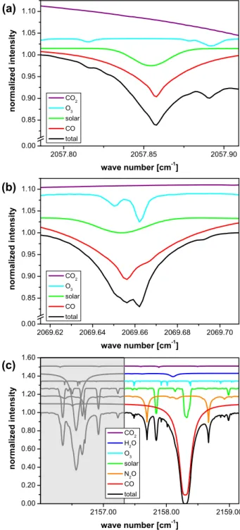
3.2.2 Contribution plot and forward model characteristics In the following we will characterize the standard CO re-trieval using the microwindow set given by Rinsland et al. (2000) (2057.78–2057.91 cm−1, 2069.61–2069.71 cm−1, and 2157.30–2159.15 cm−1). Figure 1 shows a contribution
plot (colored lines). It has been calculated using the aver-age SZA and the averaver-age of the retrieved states ˆxi of our
test ensemble. Note that there are four terrestrial interfering species, i.e., O3, H2O, N2O, and CO2. Furthermore, it can
be seen that the residual problem found between 2157.77– 2157.92 cm−1(as mentioned in Sect. 3.2.1) is due to a solar CO line that has not been adequately modeled.
For the forward simulations we used the HITRAN 2004 spectroscopic line parameter compilation (Rothmann et al., 2005). For the pressure-temperature profile information used in the forward model we utilized the daily Munich radio sonde launched at 12:00 universal time about 80 km north of the Zugspitze.
(c)
(b)
2157.00 2158.00 2159.00 0.00 0.20 0.40 0.60 0.80 1.00 1.20 1.40 1.60 n o rm a li z e d i n te n s it y wave number [cm-1] CO2 H2O O3 solar N2O CO total 2069.62 2069.64 2069.66 2069.68 2069.70 0.00 0.85 0.90 0.95 1.00 1.05 1.10 n o rm a li z e d i n te n s it y wave number [cm-1] CO2 O3 solar CO total 2057.80 2057.85 2057.90 0.00 0.85 0.90 0.95 1.00 1.05 1.10 n o rm a li z e d i n te n s it y wave number [cm-1] CO2 O3 solar CO total(a)
Fig. 1. Forward calculation of the three micro-windows (a–c) of the
solar infrared absorption spectrum used for CO profile retrievals. The contributions of the different absorbing species are separated. Note, that the grey-shaded spectral area in (c) is not used for the standard retrieval. It is only used for the sensitivity study with the widened microwindow in Sect. 5.1.
3.3 The standard CO retrieval settings
We use the SFIT2 (ver. 3.90) software with an equidistant 1-km-layer retrieval grid for the target species and follow
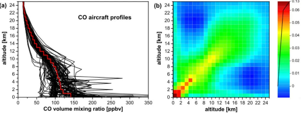
0 2 4 6 8 10 12 14 16 18 20 22 24 0 50 100 150 200 250 300 350 CO aircraft profiles
CO volume mixing ratio [ppbv]
a lt it u d e [ k m ] (b) 0 2 4 6 8 10 12 14 16 18 20 22 24 0 2 4 6 8 10 12 14 16 18 20 22 24 altitude [km] a lt it u d e [ k m ] - -0.01 - 0 - 0.01 - 0.02 - 0.03 - 0.04 - 0.05 - 0.06 - 0.13 (a)
Fig. 2. Climatological ensemble of CO aircraft profiles used to construct the Zugspitze CO a priori profile (a) and the CO a priori covariance (b). Note, that the units of the state vector are scaling factors for the VMR-layer averages of the a priori profile given on a 1 km grid.
2.964 4 6 8 10 12 14 16 18 20 22 24 0 50 100 150 200 250 300
Zugspitze a priori ensemble (aircraft) retrieved ensemble (Zugspitze FTIR)
CO volume mixing ratio [ppbv]
a lt it u d e [ k m ]
Fig. 3. CO profiles retrieved via optimal estimation from a test
en-semble of 156 Zugspitze solar FTIR spectra plotted together with the climatological aircraft profile ensemble used to construct the a priori information (see also Fig. 2). The CO standard retrieval in-cluding a VMR-profile scaling retrieval for all interfering species has been used with the Rinsland et al. (2000) microwindows.
the RRC retrieval approach as described by Rinsland et al. (2000) and Rodgers and Connor (2003), with the modi-fications that follow.
3.3.1 CO a priori profile and full covariance for mid lati-tudes
To extend the RRC approach, we used a full CO a priori co-variance matrix for the Zugspitze retrievals. This matrix was constructed from an ensemble of measured high-resolution profiles. Earlier RRC had used a simple empirical a priori co-variance matrix for CO comprising diagonal elements only, with the standard deviations (stdv) for all layers either varied smoothly from 40% below 30 km to 20% above 40 km (Rins-land et al., 2000), or all set to 100% (Rodgers and Connor, 2003). While these RRC retrieval settings were an empirical
approach to stabilize the retrieval without too much influence from a priori information, the Zugspitze approach employs a strict application of the optimal estimation concept to the re-trieval of CO profiles from solar FTIR.
The Zugspitze a priori profile ta and a priori covariance
matrix St=SCOfor optimal estimation of CO was constructed
from an ensemble of globally distributed aircraft CO mea-surements supplemented above the aircraft altitudes by a set of modeled profiles used for the operational MOPITT re-trieval (Deeter et al., 2003). We selected a subset comprising all profiles within a full 47◦N±16◦latitudinal band (Fig. 2a). Figure 2a also shows the mean profile of this ensemble which is used as an a priori profile ta. The resulting a priori
covari-ance matrix St=SCOwas calculated from the statistics of the
ensemble (Fig. 2b).
3.3.2 Error covariance Sεand deweighting
The measurement error covariance matrix Sε was assumed
to be diagonal. For the uncertainties of all spectral channels the average signal-to-noise ratio of the Zugspitze test ensem-ble was used (377:1). To prevent the forward model error around 2157.77–2157.92 cm−1 (see Sects. 3.2.1 and 3.2.2) from being mapped into the retrieval, we performed a total deweighting by assuming a signal-to-noise ratio of 0:1 for this spectral domain within the Sεmatrix.
3.3.3 Retrieval of interfering species and auxiliary scalar parameters
In the standard RRC approach all four interfering species are retrieved via VMR-profile scaling. The following auxiliary scalar parameters were retrieved. There is one independent frequency shift per microwindow (i.e., 3 parameters in total). One additional parameter is needed to fit possible zero line distortions via the saturated R3 line. Three more parameters are used to fit the background slope in each micro-window. There is also one auxiliary parameter to fit a frequency shift to the solar CO spectrum.
0 1 4 6 8 10 12 14 16 18 20 22 24 2.9644 6 8 10 12 14 16 18 20 22 24 0.0 0.2 0.4 24.5 km 13.5 km 23.5 km 12.5 km 22.5 km 11.5 km 21.5 km 10.5 km 20.5 km 9.5 km 19.5 km 8.5 km 18.5 km 7.5 km 17.5 km 6.5 km 16.5 km 5.5 km 15.5 km 4.5 km 14.5 km 3.5 km
averaging kernel
a
lt
it
u
d
e
[
k
m
]
area
Fig. 4. Averaging kernels (rows of the averaging kernel matrix) forthe Zugspitze standard retrieval of CO profiles via optimal estima-tion. The nominal altitudes of the kernels are given as well as the areas of the kernels as a function of altitude (black curve in the right part). The CO standard retrieval including a VMR-profile scaling retrieval for all interfering species has been used with the Rinsland et al. (2000) microwindows. The kernels plotted are the average of the kernels calculated around all states retrieved from the Zugspitze test ensemble of 156 spectra. Note, that the units of the state vector are scaling factors for the VMR-layer averages of the a priori profile given on a 1 km grid.
3.3.4 Retrieved test ensemble
Figure 3 shows the retrieved CO profiles from an arbitrar-ily chosen test ensemble of 156 Zugspitze spectra. It can be seen that the overall range of scatter of the retrieved ensem-ble is consistent with the ensemensem-ble of the aircraft profiles (also shown) from which our prior information (covariance and mean profile) was constructed.
3.4 Quantification of CO smoothing error
Averaging kernels for the standard CO profile retrieval (i.e., the rows of At t=ACO−CO, see Eq. 4) are plotted in Fig. 4. The
plotted averaging kernels are averages of the averaging ker-nels calculated around all the retrieved states of the Zugspitze test ensemble (Fig. 3), i.e., they describe the mean retrieved state. The kernels peak close to their nominal altitude and re-tain close to unit area up to an altitude of 15 km. The degree of freedom of signal is dofs = 3.3 on average over our test ensemble.
We calculate the smoothing error covariance St t=SCO−CO
according to Eq. (8) using the a priori covariance St=SCOof
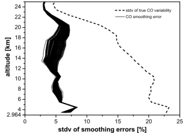
Fig. 2b. Figure 5 shows the square roots of the diagonal
el-2.9644 6 8 10 12 14 16 18 20 22 24 0 5 10 15 20 25 stdv of true CO variability CO smoothing error stdv of smoothing errors [%] a lt it u d e [ k m ]
Fig. 5. Profile of the stdv of the true CO variability (dashed line:
square roots of the diagonal elements of the climatological CO co-variance) and ensemble of smoothing error profiles (solid lines: square roots of the diagonal elements of the smoothing error co-variance) calculated around all states retrieved from the Zugspitze test ensemble of 156 spectra. The CO standard retrieval including a VMR-profile scaling retrieval for all interfering species has been used with the Rinsland et al. (2000) microwindows.
ements of SCO−CO, i.e., error standard deviations as profiles
versus altitude. Note that this is not a complete description of the smoothing errors, because they are correlated between different heights. However, it does provide an indication of the retrieval precision. Figure 5 shows the full ensemble of smoothing error profiles calculated around each retrieved state (ˆxi, bi) of the Zugspitze test ensemble. As described in
Sect. 2.3, the reason for the spread of the smoothing errors is the non-linearity of the forward model and thus the depen-dency of the averaging kernels on the state (xi, bi). We found
that the major impact is due to the changing SZA.
Figure 5 also shows the natural CO variability as a func-tion of altitude which has been calculated as the square root of the diagonal elements of the a priori covariance St=SCO
(Fig. 2b). It can be seen that the magnitude of the smooth-ing error relative to the natural CO variability increases with altitude. However, the smoothing error of our retrieval never exceeds the magnitude of the natural CO variability, as ex-pected for a properly set optimal estimation approach. 3.5 Quantification of interference errors for the CO
stan-dard retrieval
The interference error covariances SCO−O3, SCO−H2O, SCO−N2O, and SCO−CO2 are calculated hereafter according
to Eq. (9). As an input to this we first have to calculate the interference kernel matrices ACO−O3, ACO−H2O, ACO−N2O,
and ACO−CO2 (Sect. 3.5.1). The second set of inputs to
Eq. (9) are the a priori covariances for the interfering species
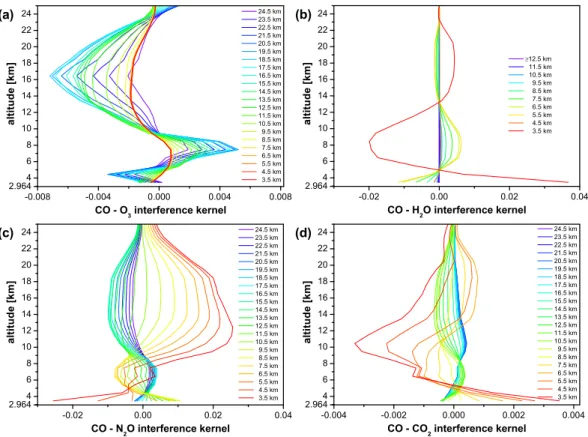
(d) (c) (b) 2.9644 6 8 10 12 14 16 18 20 22 24 -0.008 -0.004 0.000 0.004 0.008 24.5 km 23.5 km 22.5 km 21.5 km 20.5 km 19.5 km 18.5 km 17.5 km 16.5 km 15.5 km 14.5 km 13.5 km 12.5 km 11.5 km 10.5 km 9.5 km 8.5 km 7.5 km 6.5 km 5.5 km 4.5 km 3.5 km CO - O3 interference kernel a lt it u d e [ k m ] 2.964 4 6 8 10 12 14 16 18 20 22 24 -0.02 0.00 0.02 0.04 24.5 km 23.5 km 22.5 km 21.5 km 20.5 km 19.5 km 18.5 km 17.5 km 16.5 km 15.5 km 14.5 km 13.5 km 12.5 km 11.5 km 10.5 km 9.5 km 8.5 km 7.5 km 6.5 km 5.5 km 4.5 km 3.5 km CO - N 2O interference kernel a lt it u d e [ k m ] 2.9644 6 8 10 12 14 16 18 20 22 24 -0.02 0.00 0.02 0.04 ≥12.5 km 11.5 km 10.5 km 9.5 km 8.5 km 7.5 km 6.5 km 5.5 km 4.5 km 3.5 km CO - H2O interference kernel a lt it u d e [ k m ] 2.964 4 6 8 10 12 14 16 18 20 22 24 -0.004 -0.002 0.000 0.002 0.004 24.5 km 23.5 km 22.5 km 21.5 km 20.5 km 19.5 km 18.5 km 17.5 km 16.5 km 15.5 km 14.5 km 13.5 km 12.5 km 11.5 km 10.5 km 9.5 km 8.5 km 7.5 km 6.5 km 5.5 km 4.5 km 3.5 km CO - CO 2 interference kernel a lt it u d e [ k m ] (a)
Fig. 6. Interference kernels (rows of the interference kernel matrices) for the interfering species O3(a), H2O (b), N2O (c), and CO2(d). The
kernels are calculated for the CO standard retrieval with the Rinsland et al. (2000) microwindows and a VMR-profile scaling retrieval for all interfering species. The nominal altitudes of the kernels are given. The interference kernels plotted are the average of the kernels calculated around all states retrieved from the Zugspitze test ensemble of 156 spectra. Note, that the units of the state vector are scaling factors for the VMR-layer averages of the a priori profiles given on a 1 km grid.
presented in Sect. 3.5.2. Then Sect. 3.5.3 shows the result-ing interference errors versus altitude and their comparison to the smoothing errors as well as to the natural variability of CO.
3.5.1 Interference kernels
The interference kernels for the four interfering species are plotted in Figs. 6a–d. They characterize the standard RRC retrieval which uses a 1-layer coarse-grid retrieval for the four interfering species (VMR-profile scaling). In order to be able to calculate these interference kernels via Eqs. (3, 4) we emulated this 1-layer grid on a fine retrieval grid as ex-plained in Sect. 2.2.2. For this purpose we implemented for the interfering species the same equidistant 1-km-layer re-trieval grid as used for the CO (target species) rere-trieval, and applied for their retrieval regularization matrices as given in Eq. (10) with α=1013.
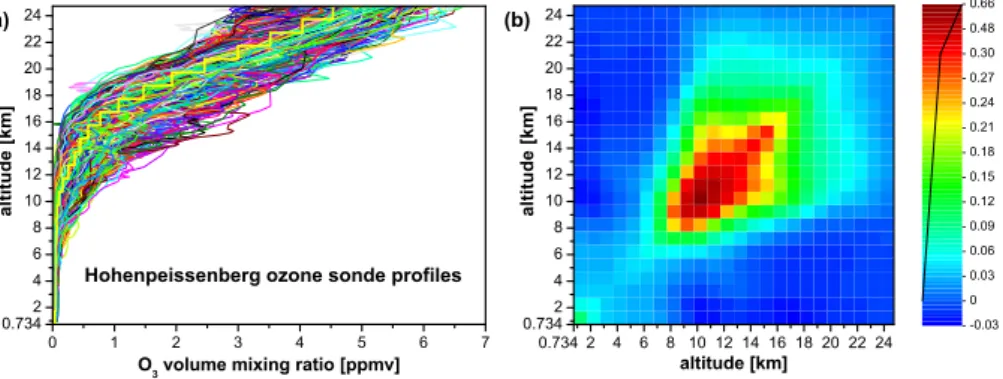
3.5.2 A priori covariances of the interfering species To construct the a priori covariance Sv1=SO3needed to
es-timate the CO-O3 interference error we used an ensemble
of 1438 ozone sonde (brewer mast) profiles provided by the meteorological observatory Hohenpeissenberg located 30 km north of the Zugspitze. These soundings are performed 3 times a week, and our ensemble covers the time span January 1995–February 2006. Figure 7a shows the profile ensemble and its mean, and Fig. 7b shows the covariance calculated from this ensemble.
To construct the a priori covariance Sv2=SH2Owe utilized
the data set of the (4 times daily) radio soundings performed during the Garmisch AIRS validation campaign between 19 August–17 November 2002. Garmisch is located horizon-tally only 6 km away from the Zugspitze. We used a subset of 66 radio sondes that had been launched coincident to the solar FTIR measurements (i.e., filtering for clear sky condi-tions). This ensemble of water vapor profiles and the result-ing covariance is plotted in Fig. 8.
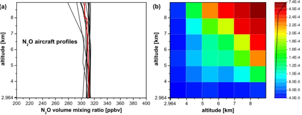
To estimate the a priori covariance Sv3=SN2Owe used an
ensemble of 14 aircraft profiles from a number of campaigns performed from 1995–1997 between 20–70◦N which were provided by the ETHmeg data base (http://www.megdb.ethz. ch/dbaccess.php), see Fig. 9.
The a priori covariance Sv4=SCO2 was constructed from
(b) 0.734 2 4 6 8 10 12 14 16 18 20 22 24 0.734 2 4 6 8 10 12 14 16 18 20 22 24 altitude [km] a lt it u d e [ k m ] - -0.03 - 0 - 0.03 - 0.06 - 0.09 - 0.12 - 0.15 - 0.18 - 0.21 - 0.24 - 0.27 - 0.30 - 0.48 - 0.66 0.734 2 4 6 8 10 12 14 16 18 20 22 24 0 1 2 3 4 5 6 7
O3 volume mixing ratio [ppmv]
a lt it u d e [ k m ]
Hohenpeissenberg ozone sonde profiles
(a)
Fig. 7. Climatological ensemble of ozone sonde profiles used to construct the Zugspitze O3a priori profile (a) and the O3climatological covariance (b). Note, that the units of the state vector are scaling factors for the VMR-layer averages of the a priori profile given on a 1 km grid. 0.734 2 4 6 8 10 12 14 0.000 0.005 0.010 0.015
H2O volume mixing ratio
a lt it u d e [ k m ]
Garmisch radio sonde profiles
(b) 0.734 2 4 6 8 10 12 14 0.734 2 4 6 8 10 12 14 altitude [km] a lt it u d e [ k m ] - 0 - 0.05 - 0.10 - 0.15 - 0.20 - 0.25 - 0.30 - 0.35 - 0.40 - 0.44 (a)
Fig. 8. Climatological ensemble of radio sonde profiles used to construct the Zugspitze H2O a priori profile (a) and the H2O climatological covariance (b). Note, that the units of the state vector are scaling factors for the VMR-layer averages of the a priori profile given on a 1 km grid.
July/August 2000 and May/June 2003 between 31–56◦N. This data was provided by the ETHmeg data base, see Fig. 10.
3.5.3 Resulting interference errors for the CO standard re-trieval
Based on the results of Sects. 3.5.1 and 3.5.2 the interfer-ence error covariances SCO−O3, SCO−H2O, SCO−N2O, and SCO−CO2 were calculated according to Eq. (9). In analogy
to Fig. 5 we plotted the square roots of the diagonal elements of the interference error covariances as profiles versus alti-tude, see Fig. 11b for the standard retrieval (VMR-profile scaling retrieval of the interfering species) using the Rins-land et al. (2000) microwindows. Again, as for the smooth-ing error, we plotted the full ensemble of interference errors versus altitude calculated around each of the retrieved states of the Zugspitze test ensemble. The spread of the interfer-ence error profiles of one species is due to non-linear effects (mainly due to changing SZA) as discussed in Sect. 2.3 in general and in Sect. 3.4 for the case of smoothing errors. Figure 11b illustrates a crucial result of this paper, namely,
that interference errors can be significant, i.e., they can be as high as smoothing errors, or even exceed them: CO-O3
in-terference errors frequently exceed the CO smoothing error in the altitude range between ≈14–19 km, and CO-H2O
in-terference errors are comparable to the CO smoothing errors in the lower troposphere. We note that the Zugspitze is a dry site and CO-H2O interference errors would be even higher
for low altitude sites.
Figure 4 in Rodgers and Connor (2003) should be com-parable with our Fig. 11b since both figures display inter-ference errors and smoothing errors of the standard ground-based FTIR retrieval of CO profiles. However, the interfer-ence errors shown in Fig. 4 of Rodgers and Connor (2003) are significantly smaller than the interference errors obtained in our work (see Fig. 11b). In other words, interference er-rors in Fig. 4 of Rodgers and Connor (2003) are more than an order of magnitude smaller than the CO smoothing error, while interference errors are comparable to the smoothing er-ror or higher in our Fig. 11b. Obviously, this underestimation of interference errors arises because interference errors were directly calculated on the coarse 1-layer grid of the standard retrieval (as explained in Sect. 7.1.2 of Rodgers and Connor,
2.964 4 5 6 7 8 200 220 240 260 280 300 320 340 360 380 400 N 2O aircraft profiles
N2O volume mixing ratio [ppbv]
a lt it u d e [ k m ] 2.964 4 5 6 7 8 2.964 4 5 6 7 8 altitude [km] a lt it u d e [ k m ] - 4.0E-5 - 6.0E-5 - 8.0E-5 - 1.0E-4 - 1.2E-4 - 1.4E-4 - 1.6E-4 - 1.8E-4 - 2.0E-4 - 2.2E-4 - 2.4E-4 - 4.5E-4 - 7.4E-4 (b) (a)
Fig. 9. Climatological ensemble of aircraft profiles used to construct the Zugspitze N2O a priori profile (a) and the N2O climatological
covariance (b). Note, that the units of the state vector are scaling factors for the VMR-layer averages of the a priori profile given on a 1 km grid. 2.964 4 5 6 7 2.964 4 5 6 7 altitude [km] a lt it u d e [ k m ] - 1.60E-4 - 1.70E-4 - 1.80E-4 - 1.90E-4 - 2.00E-4 - 2.10E-4 - 2.20E-4 - 2.30E-4 - 2.40E-4 - 2.48E-4 (b) 2.964 4 5 6 7 330 340 350 360 370 380 390 400 Jul/Aug '00 May/Jun '03 mean profile
CO2 volume mixing ratio [ppmv]
a lt it u d e [ k m ] CO 2 aircraft profiles (a)
Fig. 10. Climatological ensemble of aircraft profiles used to construct the Zugspitze CO2a priori profile (a) and the CO2climatological covariance (b). Note, that the units of the state vector are scaling factors for the VMR-layer averages of the a priori profile given on a 1 km grid.
2000), and not via a fine-grid emulation of this course grid as suggested in our Sects. 2.2.2 and 3.5.1.
4 Sensitivity studies and minimization of interference errors
4.1 Interference errors in case of unretrieved interfering species
We quantify here the interference errors for the case that the interfering species are not retrieved. Since we have already implemented the interfering species within the state vector of our algorithm on a fine retrieval grid, we can quickly switch to “non-retrieval” by using our concept of “dead regulariza-tion” according to Eq. (12).
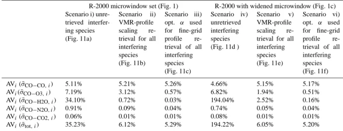
Results are shown in Fig. 11a. All interference errors have strongly increased as compared to the standard retrieval, where the interfering species are retrieved via VMR-profile scaling (Fig. 11b). This striking tendency is also documented in Table 1 via numbers, utilizing the concept of “mean er-rors” defined in Eq. (14): in Scenario i) (unretrieved
in-terfering species) the average over the i=1. . . 156 retrieved states of our Zugspitze test ensemble (AVi) of the “total
mean error” ¯σtot, i:=sqrt( ¯σCO−CO, i2 + ¯σCO−O3, i2 + ¯σCO−H2O, i2
+ ¯σCO−N2O, i2 + ¯σCO−CO2, i2 ) is AVi( ¯σtot, i)=35.23%; it is
dominated by a high water-vapor interference, AVi
( ¯σCO−H2O, i)=34.10%. Compared with this, a
VMR-profile scaling retrieval of the interfering species, reduces AVi( ¯σtot, i) from 35.23% (Scenario i) to 6.12% in
Sce-nario ii), which is now dominated by the smoothing error (5.21%), but is still significantly affected by interference, mainly due to O3(3.12%).
4.2 Effect from implementing the optimum strategy to so-lar CO retrivals
We show now that interference errors in solar CO retrievals can be practically eliminated by implementing the optimum strategy for retrieval of the interfering species as introduced in Sect. 2.4.2. This means to reduce the regularization of the retrieval of the interfering species from a simple scal-ing retrieval (which is the standard approach) towards a weakly regularized (profile) retrieval on a fine grid. This is
2.964 4 6 8 10 12 14 16 18 20 22 24 0 25 50 75
stdv of smoothing and interference errors [%]
a lt it u d e [ k m ] 2.964 4 6 8 10 12 14 16 18 20 22 24 0 25 50 75
stdv of smoothing and interference errors [%]
a lt it u d e [ k m ] 2.964 4 6 8 10 12 14 16 18 20 22 24 0 5 10 15 20 25
stdv of smoothing and interference errors [%]
a lt it u d e [ k m ] 2.9644 6 8 10 12 14 16 18 20 22 24 0 5 10 15 20 25
stdv of smoothing and interference errors [%]
a lt it u d e [ k m ] 2.964 4 6 8 10 12 14 16 18 20 22 24 0 5 10 15 20 25
stdv of smoothing and interference errors [%]
a lt it u d e [ k m ] 2.9644 6 8 10 12 14 16 18 20 22 24 0 5 10 15 20 25
stdv of smoothing and interference errors [%]
a lt it u d e [ k m ]
stdv of true CO variability CO smoothing error CO - O3 interf. error CO - H2O interf. error CO - N2O interf. error × 10 CO - CO2 interf. error × 10
(b) (c) (d) (a) (e) (f)
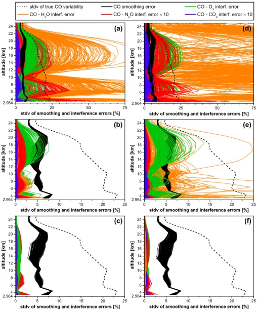
Fig. 11. Profiles of the interference errors CO-O3, CO-H2O, CO-N2O, and CO-CO2(colored curves: square roots of the diagonal elements
of the interference error covariances, black: same for smoothing error) calculated around all states retrieved from the Zugspitze test ensemble of 156 spectra. (a) Errors for the CO standard retrieval with the Rinsland et al. (2000) microwindows but the interfering species not retrieved.
(b) Errors for the CO standard retrieval with the Rinsland et al. (2000) microwindows and VMR-profile scaling retrieval of the interfering
species. (c) Rinsland et al. (2000) microwindows and optimized profile retrievals of the interfering species using the regularization parameters given in Table 2. (d) Widened microwindow (Fig. 1c) and non-retrieval of interfering species. (e) Widened microwindow (Fig. 1c) and VMR-profile scaling retrieval of interfering species. (f) Widened microwindow (Fig. 1c) and optimized VMR-profile retrievals of the interfering species using the regularization parameters given in Table 2.
accomplished by a slight increase in smoothing error, i.e., there is a tradeoff between both effects and a minimiza-tion of the combined error can be performed as explained in Sect. 2.4.2.
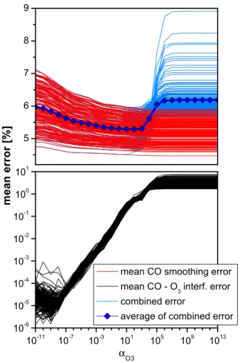
Figure 12 shows on its horizontal scale the transition from a VMR-profile scaling retrieval for O3(using the L1operator
in combination with very high values for the regularization parameter, i.e., αO3=1013) towards an essentially
unregu-larized profile retrieval (αO3=10−11). The vertical scale in
Fig. 12 shows the “mean smoothing errors” ¯σCO−CO, i (red
curves) and the “mean interference error” ¯σCO−O3, i (black
curves) as defined in Eq. (14). These errors are calculated around all i=1. . . 156 retrieved states of the Zugspitze test ensemble as a function of αO3. The ensemble-type nature
of these plots again results from the described non-linearity effects. As a result from Fig. 12 it can be seen, that the mean CO-O3interference errors decrease together with
de-creasing αO3 as expected. Figure 12 also shows that the
mean CO smoothing errors are increasing slightly with de-creasing αO3 as expected. Therefore, an optimum αO3 for
the i-th retrieval of the interfering species O3can be found