HAL Id: hal-00295549
https://hal.archives-ouvertes.fr/hal-00295549
Submitted on 22 Nov 2004
HAL is a multi-disciplinary open access
archive for the deposit and dissemination of
sci-entific research documents, whether they are
pub-lished or not. The documents may come from
teaching and research institutions in France or
abroad, or from public or private research centers.
L’archive ouverte pluridisciplinaire HAL, est
destinée au dépôt et à la diffusion de documents
scientifiques de niveau recherche, publiés ou non,
émanant des établissements d’enseignement et de
recherche français ou étrangers, des laboratoires
publics ou privés.
chemistry-climate model in comparison with
observations
H. Struthers, K. Kreher, J. Austin, R. Schofield, G. Bodeker, P. Johnston, H.
Shiona, A. Thomas
To cite this version:
H. Struthers, K. Kreher, J. Austin, R. Schofield, G. Bodeker, et al.. Past and future simulations of NO2
from a coupled chemistry-climate model in comparison with observations. Atmospheric Chemistry and
Physics, European Geosciences Union, 2004, 4 (8), pp.2227-2239. �hal-00295549�
www.atmos-chem-phys.org/acp/4/2227/ SRef-ID: 1680-7324/acp/2004-4-2227 European Geosciences Union
Chemistry
and Physics
Past and future simulations of NO
2
from a coupled
chemistry-climate model in comparison with observations
H. Struthers1, K. Kreher1, J. Austin2, R. Schofield3, G. Bodeker1, P. Johnston1, H. Shiona1, and A. Thomas1
1National Institute of Water and Atmospheric Research, Private Bag 50061, Omakau, New Zealand
2Geophysical Fluid Dynamics Lab., Princeton Forrestal Campus Rte.1, 201 Forrestal Rd., Princeton, NJ 08542-0308, USA
3NOAA Aeronomy Laboratory, 325 Broadway, R/AL8, Boulder CO 80305, USA
Received: 8 June 2004 – Published in Atmos. Chem. Phys. Discuss.: 20 August 2004
Revised: 15 November 2004 – Accepted: 15 November 2004 – Published: 22 November 2004
Abstract. Trends in NO2 derived from a 45 year
integra-tion of a chemistry-climate model (CCM) run have been
compared with ground-based NO2measurements at Lauder
(45◦S) and Arrival Heights (78◦S). Observed trends in NO2
at both sites exceed the modelled trends in N2O, the
pri-mary source gas for stratospheric NO2. This suggests that
the processes driving the NO2 trend are not solely dictated
by changes in N2O but are coupled to global atmospheric
change, either chemically or dynamically or both. If CCMs are to accurately estimate future changes in ozone, it is im-portant that they comprehensively include all processes
af-fecting NOx(NO+NO2) because NOxconcentrations are an
important factor affecting ozone concentrations. Comparison
of measured and modelled NO2trends is a sensitive test of
the degree to which these processes are incorporated in the
CCM used here. At Lauder the 1980–2000 CCM NO2trends
(4.2% per decade at sunrise, 3.8% per decade at sunset) are lower than the observed trends (6.5% per decade at sunrise, 6.0% per decade at sunset) but not significantly different at the 2σ level. Large variability in both the model and mea-surement data from Arrival Heights makes trend analysis of
the data difficult. CCM predictions (2001–2019) of NO2at
Lauder and Arrival Heights show significant reductions in the
rate of increase of NO2compared with the previous 20 years
(1980–2000). The model results indicate that the partitioning of oxides of nitrogen changes with time and is influenced by both chemical forcing and circulation changes.
Correspondence to: H. Struthers (h.struthers@niwa.co.nz)
1 Introduction
It has been recognised for some time that the reactive species
NOxare important in the altitude range from approximately
20 km to 35 km in determining the concentration of
strato-spheric ozone (Crutzen, 1970). NOxdestroys ozone through
the catalytic cycle shown in Reactions (1) and (2).
NO + O3→NO2+ O2 (1)
NO2+ O → NO + O2 (2)
(net) O3+ O → 2 O2 (3)
In the lower stratosphere (approximately 10 km to 20 km)
the most significant influence of NOxis its interaction with
the ClOx and BrOx ozone loss cycles via the formation of
reservoir species ClONO2 and BrONO2. NO2 also reacts
with OH (Eq. 4), reducing the HOxconcentration and thus
inhibiting the HOxcatalysed destruction of ozone.
NO2+OH + M → HNO3+M. (4)
Oxidation of N2O (Reaction (5)) is the
ma-jor source of stratospheric NOy (NO+NO2
+NO3+HNO3+2N2O5+HNO4+ClONO2+BrONO2) and
hence NOx(Minschwener et al., 1993).
N2O + O(1D) → 2NO. (5)
N2O concentrations are predicted to continue to increase
over the coming century due to anthropogenic surface emis-sions, mostly attributed to agricultural nitrogen fixation (IPCC, 2001; WMO, 1999). Trends in the concentration of
atmospheric N2O for the period 1980 to 1988 have been
es-timated to be +0.25±0.05% per year (IPCC (2001), p253).
per year based on remote measurements made at
Jungfrau-joch from 1984 to 1996. In contrast to N2O, stratospheric
halogen concentrations are expected to decline over the com-ing 50 years as anthropogenic emissions of halogenated ozone-depleting compounds decrease (WMO, 2003). It is therefore important to understand the combined effect of
changing halogen and NOxconcentrations on the future
evo-lution of the ozone layer.
Randeniya et al. (2002) studied the effect of increasing
N2O and methane on northern mid-latitude ozone columns
for the period 2000–2100 using the CSIRO two dimensional chemical model (Randeniya et al., 1997). Their model re-sults show partial recovery of ozone columns through to the middle of the century due to reductions in halogen concen-trations. This is followed by reduction in ozone columns from 2050 to 2100 which Randeniya et al. (2002) attribute
to increased destruction of ozone by NOx, modulated by
the amount of methane present in the model. Methane con-centrations influence the ozone recovery through the photo-oxidation of methane by halogen radicals in the lower strato-sphere and above 20 km through changes in OH concen-trations leading to changes in the rate of conversion of
NO2 to HNO3. Comparing model ozone profiles for 2100
with profiles from 2000, Randeniya et al. (2002) find in-creases in lower stratospheric ozone concentrations over the 2000–2100 integration. This is explained by a reduction in the amount of ozone destroyed by halogen catalytic cycles. However, the recovery in lower stratospheric ozone is offset by reductions of up to 7% in ozone concentrations in the
mid-dle stratosphere due to increased NOxcatalytic destruction of
ozone.
Modelling future ozone change requires realistic
repre-sentations of the anticipated changes in NOx and halogens,
in addition to the many other interacting chemical and
dy-namical components of the stratospheric system.
Three-dimensional coupled chemistry-climate models (CCMs) are designed to capture the interaction between climate change and changes in atmospheric chemistry and are now becom-ing important tools in the prediction of future stratospheric chemistry and dynamics (WMO, 2003). To have confidence in CCM predictions of future stratospheric change, it is nec-essary to assess their reliability. An important methodology for validating components of atmospheric chemical models is comparison of long time-series of modelled and measured amounts of trace gases.
Since climate models underpinning all CCMs are chaotic and exhibit unforced variability, comparisons of CCM output with observations are necessarily statistical in nature. Al-though comparisons between CCM output and observations on individual days are not meaningful in anything other than a climatological sense, the response of the model to long term forcings should agree with the response observed in the real atmosphere. For this reason, long time-series of observa-tions are required to compare the modelled response to at-mospheric forcings (WMO, 2003).
High quality measurements of NO2 slant column
den-sities have been routinely made at Lauder, New Zealand
(45◦S) since 1980 (Johnston and McKenzie, 1989) and
Arrival Heights, Antarctica (77.8◦S) since 1982
(McKen-zie and Johnston, 1984; Keys and Johnston, 1986, 1988). The measurements are taken at twilight (sunrise and
sun-set). Measuring at a solar zenith angle (SZA) of 90◦ with
zenith sky viewing geometry increases the sensitivity of the
observed columns to stratospheric NO2amounts (Solomon
et al., 1987).
Liley et al. (2000) studied the Lauder NO2data set using
least squares regression. Indices of QBO, ENSO, solar cycle and the El Chichon and Pinatubo volcanic events in
addi-tion to the NO2annual cycle and secular trend were fitted to
the measured NO2time-series. Liley et al. (2000) concluded
that the mean 90◦SZA linear trend in NO
2over Lauder from
1980 to 1999 was 5±1% per decade (sunrise trend 5.9±2.4, sunset trend 4.6±1.5 % per decade). These trends are
signifi-cantly greater than the trend in N2O estimated to be between
2.5% and 3.3% per decade (WMO, 1999). As N2O is the
dominant source of stratospheric NO2, this result implies that
there has been a dynamical or chemical change at southern
mid-latitudes which has increased NO2disproportionately.
Using 1995–2002 Fourier Transform Infra-Red (FTIR)
measurements at Kitt Peak (31.9◦N), Rinsland et al. (2003)
derived an NO2trend of 10.3±5.5% (2σ ) per decade. Liley
et al. (2000) show however, that using short time periods in regression analyses results in large uncertainties in the trends and therefore the results of Rinsland et al. (2003) cannot be meaningfully compared with those of Liley et al. (2000)
or those presented here. NO2 data derived from a
com-bination of FTIR and differential optical absorption spec-troscopy measurements taken at the Network of the Detec-tion of Stratospheric Change (NDSC) staDetec-tion at
Jungfrauo-joch (46.5◦N) have been analysed and suggest a linear
increase for the period 1985–2001 of 6±2% per decade
(WMO, 2003). These results suggest that the NO2trend
be-ing greater than the N2O trend is unlikely to be a local feature
at Lauder but is likely to be of global extent.
Fish et al. (2000) used a column model to determine the
sensitivity of southern mid-latitude NO2to changes in
strato-spheric temperature, ozone and water vapour. A number of
possible mechanisms that could change the amount of NO2
relative to the amount of N2O were identified:
– direct emission of NOx
– changes in stratospheric circulation
– changes in the shape of the mean NO2profile – changes in the partitioning of NOy.
Changes in the partitioning of NOy could arise due to
changes in ozone, temperature, stratospheric water vapour and sulfate aerosol. The focus of Fish et al. (2000) was
could explain the observed trend in NO2. The model was
forced with observed changes in ozone, temperature and
wa-ter vapour and a 2.5% per decade increase in N2O. The model
failed to reproduce the observed NO2 trend (model trends
+4.0±0.6% per decade at sunrise, +2.0±0.4% per decade at sunset). Including a 20% decrease in stratospheric aerosol
in the model forcing gave NO2trends in agreement with
ob-servations (model trends +5.9±0.6% per decade at sunrise, +4.3±0.4% per decade at sunset).
McLinden et al. (2001) used a combination of a three-dimensional chemical transport model, a static column chemistry model and a radiative transfer model to generate
NO2slant column densities and compared the change in the
columns over a 20 year time period with the Lauder NO2
ob-servations. Their results show a trend in NO2of 4.3% per
decade for a prescribed increase in N2O of 3% per decade.
Differences in the trends of NO2and N2O were attributed to
the less than equivalent conversion of N2O to NOyand
repar-titioning of NOydue to ozone and halogen changes. The
sen-sitivity of their system to temperature and aerosol changes was also investigated. McLinden et al. (2001) show that the
trend in NO2 vertical column density varies diurnally with
large changes in the slant column density trends at sunrise and sunset.
Both the studies of Fish et al. (2000) and McLinden et al. (2001) do not explicitly model the influence of circulation
changes on NO2amounts. They use rather different models
and forcings to estimate NO2 slant column density trends.
Both conclude that their models reproduce the observed NO2
trend but differ in their conclusion as to why there is a
dis-tinction between the trends in NO2and N2O. More work is
required to fully understand the mechanisms responsible for the observed difference in trends.
In this paper we calculate NO2slant column densities for
Lauder and Arrival Heights using results from the Unified Model with Eulerian Transport and Chemistry (UMETRAC),
a three-dimensional CCM. NO2values are derived from a 40
year simulation of the model, (1980 to 2019). Model NO2
slant columns for Lauder and Arrival Heights are compared with the measurements for the period 1980 to 2000 to test the model’s ability to reproduce the greater than than
pro-portional increase in NO2relative to N2O that has been
ob-served in the measurements. The UMETRAC predictions of
NO2trends at Lauder and Arrival Heights for the period 2001
to 2019 are introduced and discussed in light of the 1980 to 2000 model/observation comparison.
2 Measurements
The NO2 measurement technique and retrieval algorithm
are discussed by Johnston and McKenzie (1989) and Liley et al. (2000). The automated scanning spectrometers mea-sure wavelengths from 435 nm to 450 nm with a spectral res-olution of 1.2 nm. Twilight spectra are ratioed with
mid-day reference spectra to remove Fraunhofer absorption lines present in sunlight. Each twilight measurement is also cor-rected for the Ring effect (Grainger and Ring, 1963) using the “offset Ring” approach (Johnston and McKenzie, 1989). The instruments at Lauder and Arrival Heights have been calibrated and intercompared to the standard required of the Network for Detection of Stratospheric Change (NDSC).
Model ozone and 20 hPa temperatures are also compared with measurements as changes in these quantities have been identified by Fish et al. (2000) and McLinden et al. (2001) as
being important in determining changes in NO2. The 20 hPa
level approximately coincides with the peak in the NO2
mix-ing ratio and was therefore used as the level for the temper-ature comparison. It has been shown (Keys and Johnston,
1986) that NO2slant columns measured over Arrival Heights
correlate strongly with stratospheric temperatures.
Modelled ozone data are compared with the NIWA assim-ilated ozone data-set (Bodeker et al., 2001). This data-set contains total column ozone values derived from a combina-tion of TOMS and GOME satellite measurements which are corrected against the global ground-based network of Dob-son spectrophotometers. NCEP/NCAR (Kalnay et al., 1996) 20 hPa temperature data are used for the temperature com-parison.
3 Least squares regression analysis
Linear trends in the NO2 slant column density time-series
are calculated using a least squares regression model. The regression model has been applied to ozone time-series in previous studies (Bodeker et al., 1998, 2001).
A number of forcings are known to influence the southern mid-latitude stratosphere:
– El Ni˜no southern oscillation (ENSO) – Quasi-biennial oscillation (QBO) – 11 year solar cycle
– Volcanic injection of sulfate aerosol and water vapour. For the time period 1980–2000, two volcanic events occurred which were significant for the southern mid-latitude stratosphere, El Chichon (1982) and Pinatubo (1991).
The regression model is designed to allow fitting of indices for the above forcings, in addition to fitting the seasonal cycle and linear trend in the data. Inclusion of additional, higher order Fourier components to the basis function describing the trend allows the model to fit seasonally varying trends in the data. A description of the indices for the externally forced basis functions (ENSO, QBO, solar cycle and volca-noes) within the regression model is given in Bodeker et al. (1998).
The residual terms from the fitting may be autocorrelated leading to an underestimation of the uncertainty in the re-sulting trends. An autocorrelation model is applied to the residuals to correct for any autocorrelation.
For the observational record, all basis functions (ENSO, QBO, solar cycle volcanoes) are included in the regres-sion analysis. For the model time-series, only the ENSO and QBO terms are applied (in addition to the annual cy-cle (offset) and linear trend). The model does not include an 11 year solar cycle and uses an invariant, background sul-fate aerosol field. The non-orographic gravity wave forcing scheme within the model produces a QBO in the tropical zonal winds (Scaife et al., 2000). Mean, equatorial zonal winds produced by the model at 50 hPa were used to gener-ate the model QBO basis function.
4 Model description
4.1 The coupled chemistry-climate model
UMETRAC uses the Met Office’s Unified Model (UM) (Cullen and Davies, 1991) as the underlying climate model.
The model has a resolution of 3.75◦ (longitude), 2.5◦
(lat-itude) and 64 vertical levels from the surface to 0.01 hPa. A non-orographic gravity wave forcing scheme (Warner and McIntyre, 1999) is used to parameterise gravity wave break-ing.
The UMETRAC chemistry scheme is based on a families approach (Austin, 1991). 15 chemical tracers and one dy-namical tracer are advected by the model. The dydy-namical
tracer is used to parameterise the long lived species H2O,
CH4, Cly, Bry, H2SO4 and NOy. The chemistry scheme
includes 65 gas phase chemical reactions, 9 heterogeneous
chemical reactions and 27 photolysis reactions. A PSC
scheme based on liquid ternary solutions and water ice and a simple sedimentation scheme are also part of the model. Chemical reaction rates are taken from DeMore et al. (1997) and Sander et al. (2000).
There are some differences between the UMETRAC con-figuration used in this paper and the concon-figuration used in previous work (Austin and Butchart, 2003). These include a new tracer advection scheme, the chemistry scheme being applied over the whole vertical domain of the model rather than being restricted to the stratosphere and lower meso-sphere, two additional chemical tracers are included (CO and
CH3OOH) and an extension of the chemical reaction set.
Water vapour concentrations in the chemistry module were taken from the UARS reference atmosphere project (URAP) reference atmosphere (http://code916.gsfc.nasa.gov/Public/ Analysis/UARS/urap/home.html) and held fixed over the in-tegration. Stratospheric aerosol was derived from the aerosol surface area densities given in Table 8.8 of WMO (1991). Again, the aerosol amounts were held constant over the model integration.
Importantly for this study, the rate of increase of N2O was
fixed at +2.6% per decade for the entire length of the inte-gration (1980 to 2019). The model uses a parameterisation
to determine the amount of NOypresent at each time step,
based on the transport of a conserved tracer and the com-pact relationships of Plumb and Ko. (1992). In a subsequent
step, the model partitions the NOyaccording to the
chemi-cal scheme within the model. The global rate of increase of
NOyis fixed to the rate of increase in N2O (2.6% per decade)
but local rates of increase in NOymay differ from this in
re-sponse to circulation changes in the model via changes in the conserved tracer.
Results used in this paper come from a 45 year integration of UMETRAC (1975 to 2019), with the first five years used as model spinup. The IS92a IPCC scenario was used to
deter-mine greenhouse gas concentrations (CO2, CH4and N2O).
Halogen concentrations were taken from the WMO (1999) assessment. Observed sea surface temperatures (SST) were used in the model from 1975 to 1999. For years after 1999, sea surface temperature data were taken from simulations of a coupled ocean-atmosphere version of the UM.
Global fields of the 15 chemical tracers, 6 long-lived species and chemical families and temperature are output from UMETRAC every five days at 00:00 UT. These data are used as input for the UMETRAC column model which
produced NO2profiles.
4.2 UMETRAC column model
Since the output from the 45 year UMETRAC integration provided only concentrations of chemical families, an off-line chemical model was required to determine the parti-tioning amongst the chemical families output from the full three-dimensional model. Vertical profiles of chemical fam-ilies and daily mean temperature for the grid boxes covering Lauder and Arrival Heights were extracted from the UME-TRAC output and used as initial conditions for the column
model. The chemistry scheme within the column model
is identical to the chemical scheme used in the full three-dimensional model.
The column model was run for one day to establish the
NO2diurnal cycle. The chemical time step was reduced from
15 min in the full three-dimensional model to 3 min for the
column model. This allows NO2 profiles to be calculated
with a SZA resolution of 1◦, ensuring the diurnal cycle of
the model is adequately represented in the radiative transfer model for the calculation of slant column densities.
Over the one day integration of the column model, the
NO2concentrations will differ from the corresponding NO2
concentrations calculated in the full UMETRAC model due to the use of the diurnal mean temperature profile. Using simple sensitivity tests, it can be shown that these inconsis-tencies between the full model and the off-line column model have little impact on the slant column densities due to the
0 4 8 12 16 0 4 8 12 16 1980 1982 1984 1986 1988 1990 1992 1994 1996 1998 2000 0 4 8 12 16 N O2 s la n t co lu m n ( 1 0 1 6 m o le c cm -2) 90o pm 90o am 90o am 90o pm Aug/Sept 1988 0 4 8 12 16 N O2 s la n t co lu m n ( 1 0 1 6 m o le c cm -2) Aug/Sept 1988 Observations UMETRAC
Fig. 1. Comparison of UMETRAC modelled (black) and observed (grey) 90◦NO2slant column density time-series for Lauder (1980–
2000). Upper left panel sunrise, lower left panel sunset. A subset of the data is shown in the right hand panels to illustrate the estimated errors in the model and observed values and the data frequency.
small diurnal temperature variations in the lower and middle stratosphere where the slant column weighting is greatest.
Finally, the NO2profiles calculated by the column model
were interpolated from terrain following model levels to alti-tude surfaces from the ground to 72 km in 500 m steps.
4.3 Radiative transfer model
In transforming the measured NO2slant column densities to
vertical column densities, some prior knowledge of the verti-cal profile shape is required (McKenzie et al., 1991). Assum-ing a vertical profile shape in an air mass factor calculation can lead to errors due to the seasonal and annual variation of the true vertical profile, which the assumed profile shape may not capture. In this work the slant column densities were cal-culated using the radiative transfer model (RTM) developed by Schofield et al. (2003) from the profiles determined by UMETRAC. This allows direct comparison of slant column densities derived from UMETRAC output with observations. The RTM constructs a model atmosphere using tempera-ture, pressure and ozone profiles taken from the UMETRAC column model. The RTM uses a spherically curved atmo-spheric geometry, divided into discrete atmoatmo-spheric shells. For this study, ninety 1 km thick shells were used to
de-scribe the model atmosphere. The effects of refraction,
Rayleigh scattering, Mie scattering and molecular absorp-tion at a wavelength of 450 nm (see Sect. 2) were included
in the RTM path description of the NO2zenith-sky
measure-ment. Refractive indices were taken from Bucholtz (1995). A single scattering approximation was used for the zenith-sky viewing geometry.
The diurnal variation of the NO2profile adds complexity
to the slant column density calculation. The variation of the
NO2 abundance along the slant path with solar zenith
an-gle is explicitly taken into account. NO2 profiles at 1◦
so-lar zenith angle intervals between 30◦and 97◦calculated by
the UMETRAC column model were used to construct a two-dimensional profile grid. This was then interpolated to the relevant altitude and solar zenith angle along each scattered light path. The slant column for the solar zenith angle of
90◦ was calculated by integrating the amount of NO
2over
all light paths scattered from the zenith.
5 Discussion of Lauder results
5.1 Lauder NO2time-series
The time-series of modelled and measured NO2 slant
col-umn densities for Lauder are shown in Fig. 1. The model
re-sults capture the absolute value of the NO2slant columns and
the amplitudes of the seasonal cycle in NO2for both sunrise
and sunset very well. The model in general underestimates the observed slant columns for both the sunrise and sunset time-series. The agreement for the sunset case is somewhat worse than the sunrise which implies that the model has a
suppressed NO2diurnal cycle.
The right hand panels of Fig. 1 show a subset of the data to illustrate more clearly the data frequency and estimated er-rors. The time period (August and September 1988) was cho-sen as reprecho-sentative of the whole data record, excluding the time periods affected by the El Chichon and Pinatubo
erup-tions. Observation errors are estimated at 0.2×10¹⁶ molec
cm−2+ 5% of the observed value. This prescription comes
from an analysis of the error characteristics of the measured
spectra and the retrieval algorithm used to derive the NO2
slant column measurements.
The regression model used to fit the time-series requires an error estimate associated with each input data point. In the absence of an ab initio estimate of the error in the model
NO2 slant column densities, errors are prescribed using the
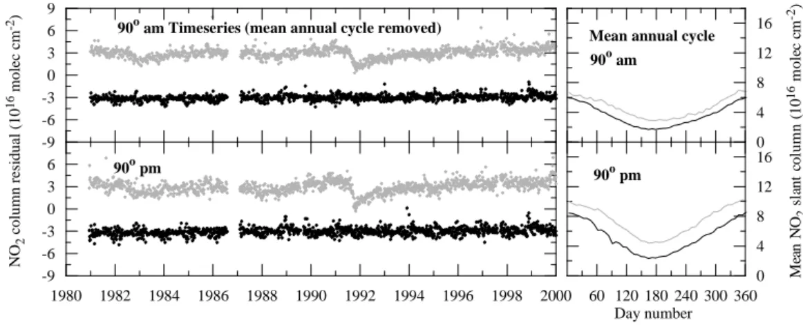
0 4 8 12 16 -9 -6 -3 0 3 6 9 1980 1982 1984 1986 1988 1990 1992 1994 1996 1998 2000 -9 -6 -3 0 3 6 N O2 c o lu m n r es id u al ( 1 0 1 6 m o le c cm
-2) Timeseries (mean annual cycle removed)
90o pm 90o am 90o am 90o pm 60 120 180 240 300 360 Day number 0 4 8 12 16 M ea n N O2 s la n t co lu m n ( 1 0 1 6 m o le c cm -2)
Mean annual cycle
Fig. 2. Lauder NO2slant column density time-series with the mean annual cycle removed. Observed residuals (grey) have been offset by
+3 units and the model residuals (black) offset by −3 units for clarity. The time-series have been thinned by retaining data only when both observation and model values are present on a given day. Right hand panels show the mean annual cycles (1980–2000) for sunrise (top) and sunset (bottom). -5 -2.5 0 2.5 5 7.5 10 L in ea r tr en d ( p e rc en t p e r d ec a d e) -5 -2.5 0 2.5 5 7.5 10 Observations (1981-2000) Model (1980-2000) Model (2000-2019) N O2 ( a m ) N O2 ( p m ) N2 O ( g lo b a l) O zo n e T em p er a tu re (K p e r d ec a d e)
Fig. 3. Seasonally independent trends in NO2for Lauder in % per
decade, derived from observations and UMETRAC model results. Also given are the estimated trends in global N2O over the same time periods and the observed and modelled trends in ozone and temperature (temperature trends are shown in K/decade). The errors are ±2σ . Note, model N2O trends are the prescribed global value
and thus has no error associated with them.
The observed data and model results from Fig. 1 were re-sampled to produce new time-series in which values were only retained for a given day, if both modelled and observed slant columns were present on that day. This processing re-moves sampling biases when comparing modelled and ob-served time-series. Figure 2 shows these time-series, with the mean annual cycles removed to show more clearly fac-tors influencing the variability in the data. For clarity, the observation and model time-series are offset by +3 and −3
(×1016molec cm−2), respectively.
The observed time-series in Fig. 2 clearly show the
reduc-tion in NO2amounts following the Pinatubo eruption. This
effect is also seen to a lesser extent for the El Chichon
erup-tion (1982). This reducerup-tion in NO2occurs via the
hydroly-sis of N2O5to HNO3on the volcanic sulphate aerosol
(Ro-driguez et al., 1991). N2O5is an important night-time NOx
reservoir and therefore removal of stratospheric N2O5causes
denoxification of the stratosphere. Other interannual vari-ability is evident in the observational record. In contrast the model results show little variation other than the short term daily variability and a linear trend.
The right hand panels of Fig. 2 show the mean annual cy-cles for the four Lauder data-sets. As indicated above, the model slant columns underestimate the observed data with the sunrise comparison being in better agreement than the sunset case. For both cases the amplitude of the modelled mean annual cycle is consistent with observations with the
whole cycle offset lower (by approximately 1×10¹⁶ molec
cm−2 for sunrise and 2×10¹⁶ molec cm−2 for sunset). A
constant shift of the modelled mean seasonal cycle NO2
rel-ative to observations suggests that too little NOyis present
in the model. This does not explain the suppression of the diurnal cycle. More work is required to fully explain the dif-ferences between the modelled and observed mean annual cycles.
5.2 Lauder past trends and factors affecting them
Seasonally independent linear trends in the observation and model time-series, calculated using the least squares analysis algorithm are given in Fig. 3.
The NO2trends derived from observations differ from the
results of Liley et al. (2000) (5% per decade) even though the same observational data-set was used in both analyses. This is because different time periods were used in the two
0 60 120 180 240 300 360 Day number -10 -5 0 5 10 15 20 N O2 t re n d ( % p er d ec ad e) 0 60 120 180 240 300 360 Day number -10 -5 0 5 10 15 20 N O2 t re n d ( % p er d ec ad e) 90oam 90opm Observations UMETRAC
Fig. 4. Annually varying NO2trends for Lauder for the period 1980–2000. The grey shaded region represents the 2σ uncertainty range in
the trends derived from model output. Error bars on the observed trends indicate ±2σ .
analyses (Liley et al. (2000) studied the period 1981–1999). The 26 parameter model with autocorrelation (AC) correc-tion used by Liley et al. (2000) for the period 1981–1999 most closely resembles the regression model used in this study. Applying our regression model to the Lauder
mea-surements for the period 1981–1999 gives linear NO2trends
that agree with the results of Liley et al. (2000).
The model NO2results underestimate the NO2trends
de-rived from the measurements for both sunrise and sunset but the model and observed trends do agree within the 2σ uncer-tainty range. The trends derived from observations are
sig-nificantly higher than the observed trends in N2O (assumed
to be between 2.5 and 3.3% per decade). This result is in agreement with the conclusions of Liley et al. (2000). The model results show a significant difference (at the 2σ level)
in the NO2 and N2O trends for the sunset case only. The
NO2results from Fig. 3 indicate that UMETRAC is not fully
capturing the magnitude of the change in relative amounts of
NO2and N2O seen in the observations over the period 1980
to 2000. This will be discussed more fully in Sect. 5.2.1
where the seasonally dependent NO2trends are examined.
Fish et al. (2000) and McLinden et al. (2001) both show
that modelled NO2trends are sensitive to changes in ozone
and temperature. Fish et al. (2000) suggest this is primarily due to the reaction,
NO2+O3→NO3+O2, (6)
which has a strong temperature dependence. To have
confi-dence in the modelled NO2 trends it is therefore important
for the model to reproduce observed ozone and temperature trends. The model slightly overestimates the seasonally in-dependent negative ozone trend (see Fig. 3) although the dif-ference from observations is within the 2σ uncertainty range. Temperature trends agree well with both the observations and model showing a small negative 20 hPa temperature trend. Both the observed and modelled temperature trends are not significantly different from zero at the 2σ level.
The NOy chemical family and HNO3 are relatively
long lived tracers in the lower stratosphere (Brasseur and
Table 1. Lauder – seasonally independent UMETRAC model
trends in NO2, N2O, ozone, temperature, NOyand HNO3for the
periods 1981–2000 and 2001–2019. Trends are given in percent per decade (temperature trends are shown in K/decade). The quoted errors are ±2σ . Model (1981–2000) Model (2001–2019) am pm am pm NO2 4.2±1.8 3.8 ±1.2 2.2±1.8 0.96±1.3 N2O 2.6 2.6 Ozone −3.3±0.7 1.3±0.8 Temperature −0.16±0.14 −0.18±0.18 NOy 2.5±1.1 2.7±1.2 HNO3 1.8±1.3 3.4±1.5
Solomon, 1986). Therefore their concentrations can be in-fluenced by both circulation changes and in-situ chemical processing. The concentrations of these species in turn
con-trol the concentration of NO2. To further investigate the role
these species have in determining trends in NO2in the model,
NOyand HNO3vertical column densities (vcds) were
calcu-lated from the model output. Every five days NOyand HNO3
vertical column densities were taken from the model output and the regression model applied to these time-series to de-termine linear trends for the period 1980–2000.
Modelled NOyand HNO3seasonally independent trends
at Lauder for the period 1980–2000 were calculated to be +2.5±1.1% per decade and +1.8±1.3% per decade,
respec-tively (Table 1). The 2.5% per decade trend in NOymatches
the global rate of increase in N2O and is significantly less
than the observed trends in NO2.
The fact that HNO3is increasing at a lower rate than NOy
suggests that the higher trend in NO2over the period 1980–
2000 is gained at the expense of HNO3, and therefore the
par-titioning in NOyover this period is shifting towards the more
chemically active NOx species and away from the HNO3
fraction of the difference between the NOyand HNO3trends
can be attributed to circulation changes and what fraction of the difference is due to chemical forcing.
5.2.1 Annually varying NO2trends
Figure 4 shows the seasonally dependent NO2trends
calcu-lated by adding two Fourier components (annual and semi-annual) to the basis function describing the trend in the re-gression model (Bodeker et al., 1998). The trends are taken as a percentage of the daily mean. That is, the trends are
cal-culated in units of molec cm−2per decade and then taken as
a percentage of the annual mean over the whole period (given in the right hand panels of Fig. 2).
The results shown in Fig. 4 indicate that for much of the
year, the model NO2trends are in good agreement with the
trends derived from observations. The greatest differences occur in spring time for both sunrise and sunset cases, where the model is underestimating the trends seen in the observa-tions. The model underestimation of the springtime increase
in NO2is the cause of the model failing to fully reproduce
the difference between the seasonally independent NO2and
N2O trends for the period 1980 to 2000 (see Fig. 3).
The same regression model (with seasonally dependent basis functions for the linear trend term) was used to fit the modelled and measured ozone and 20 hPa temperature time-series. The seasonal cycle in ozone and 20 hPa tempera-ture trends was reproduced well by the model (not shown). Therefore ozone and temperature were ruled out as the cause
of the model underprediction of springtime NO2trends.
Differences in the timing of the vortex breakup and subse-quent mixing of vortex and mid-latitude air can also be ruled out as the cause of the differences in the modelled and
ob-served Lauder springtime NO2trends. Generally, the mixing
of vortex air to mid-latitudes occurs in early summer (Ajtic, 2004), from approximately day 288 (15 October) which is after the maximum in the trend differences (approximately day 240–28 August). The model, if anything, tends to delay the breakup of the Antarctic polar vortex further reinforcing this conclusion.
Stratospheric NO2amounts have been shown to be
sen-sitive to changes stratospheric water vapour (Fish et al., 2000; McLinden et al., 2001). Measured trends in strato-spheric water vapour are uncertain (SPARC, 2000; Rosenlof et al., 2001; Randel et al., 2004). In this study, UMETRAC used a fixed climatology of stratospheric water vapour which may contribute to the discrepancy between modelled and
ob-served NO2trends.
5.3 Model predictions: Lauder 2001–2019
Table 1 (and Fig. 3) compares the seasonally independent,
predicted NO2 model trends for the period 1 January 2001
to 31 December 2019 with the model trends for the period 1 January 1980 to 31 December 2000.
Predicted NO2 trends (2001–2019) are lower than the
trends for the period 1980–2000 even though the N2O trend
stays the same. This difference is statistically significant at the 2σ level for the sunset case. Both the absolute and rela-tive differences between trends for the two periods are larger for the sunset case.
NOyand HNO3vertical column density trends for the
pe-riod 2001–2019 are compared with the 1980–2000 trends in
Table 1. It is clear from Table 1 that the shift in NO2trends
from 1980–2000 to 2001–2019 is associated with a change
in HNO3trends between the two periods. As was the case
for the 1980–2000 period, it is a change in partitioning of
the NOythat is resulting in the less than proportional rate of
increase in NO2relative to NOy(and N2O) rather than local
changes in the amount of NOyrelative to N2O.
Quantification of how chemical changes (for example halogen loading and ozone) and circulation changes affect
NOy partitioning requires additional analysis of model
re-sults which is outside the scope of this paper.
It should be reiterated that the results shown here are for
a solar zenith angle of 90◦. McLinden et al. (2001) show
that the trends in NO2 vary significantly with solar zenith
angle. It is therefore to be expected that different conclusions may be drawn from analysis of data at different solar zenith angles.
6 Discussion of Arrival Heights results
6.1 Arrival Heights NO2time-series
Arrival Heights slant column density comparisons are shown
in Fig. 5. Twilight (SZA=90◦) data at Arrival Heights are
only available during the autumn (17 February to 21 April) and spring (22 August to 25 October). Because of the large annual cycle, daily and seasonal variability and the discon-tinuous nature of the data, it is difficult to assess the level of agreement in the data from Fig. 5.
Figure 6 shows the processed Arrival Heights time-series comparison with the annual mean removed (see Sect. 5.1 and Fig. 2). Significantly less data are available for Arrival Heights than for Lauder because of the limited period of twilight (spring and autumn) at Arrival Heights and gaps in the observation record, particularly in the years 1982–1989. Both the observed and modelled data for Arrival Heights show greater variability about the mean than the Lauder data. There is good qualitative agreement between observations and model for the mean seasonal cycle at both sunrise and sunset. However, during autumn, the model tends to system-atically underpredict the observations, possibly for reasons discussed in Sect. 7.
6.2 Arrival Heights NO2trends
Regression analysis of the Arrival Heights data is compli-cated by the discontinuous nature of the data. We analyse the
0 4 8 12 16 0 4 8 12 16 1980 1982 1984 1986 1988 1990 1992 1994 1996 1998 2000 0 4 8 12 16 N O2 s la n t co lu m n ( 1 0 1 6 m o le c cm -2) 90o pm 90o am 90o am 90o pm Aug/Sept 1988 0 4 8 12 16 M ea n N O2 s la n t co lu m n ( 1 0 1 6 m o le c cm -2) Aug/Sept 1988 Observations UMETRAC
Fig. 5. Comparison of UMETRAC modelled (black) and observed (grey) 90◦NO2slant column density time-series for Arrival Heights
(1980–2000). Upper left panel sunrise, lower left panel sunset. A subset of the data is shown in the right hand panels to illustrate the estimated errors in the model and observed values and the data frequency.
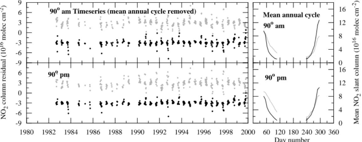
0 4 8 12 16 -9 -6 -3 0 3 6 9 1980 1982 1984 1986 1988 1990 1992 1994 1996 1998 2000 -9 -6 -3 0 3 6 N O2 c o lu m n r es id u al ( 1 0 1 6 m o le c cm
-2) Timeseries (mean annual cycle removed)
90o pm 90o am 90o am 90o pm 60 120 180 240 300 360 Day number 0 4 8 12 16 M ea n N O2 s la n t co lu m n ( 1 0 1 6 m o le c cm -2)
Mean annual cycle
Fig. 6. Arrival Heights NO2slant column density time-series with the mean annual cycle removed. Observed residuals (grey) have been
offset by +3 units and the model residuals (black) offset by −3 units for clarity. The time-series have been thinned by retaining data only when both an observation and model value is present on a given day. Right hand panels show the mean annual cycles (1980–2000) for sunrise and sunset.
autumn and spring data separately as the chemical and dy-namical regimes during the two seasons are markedly
differ-ent and therefore the NO2response is expected to be different
for the two seasons. No seasonal components were included as part of any of the basis functions used in the regression model.
The basis function describing the effect of the El Chichon eruption was not used in the regression analysis of the Ar-rival Heights data because the first observation available is 30 August 1982, approximately five months after the El Chi-chon eruption. The El ChiChi-chon basis function would include only a decay term and can potentially induce spurious trend results if included.
Because the NO2slant columns are correlated with 20 hPa
temperature, particularly in the spring (Keys and Johnston, 1986), an additional basis function was added to the regres-sion model which describes 20 hPa temperature anomalies
over Arrival Heights. Eposidic events of anomalously cold stratospheric air over Arrival Heights are associated with transport of air from the cold vortex core to Arrival Heights, which generally sits below the relatively poorly mixed edge of the polar vortex.
The temperature basis function was generated by tak-ing daily Arrival Heights 20 hPa temperatures from the NCEP/NCAR reanalysis data-set and fitting them using the
same regression model as is used for the NO2data. The
resid-ual temperatures from this fitting were then used as the
tem-perature basis function for the regression analysis of the NO2
data. The same process was applied to the model 20 hPa tem-peratures to generate the model temperature basis function.
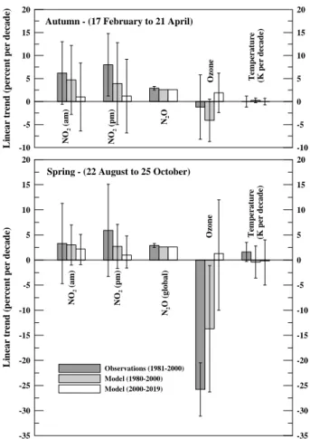
Figure 7 gives the linear, (autumn–upper panel and spring–
lower panel) trends in NO2, N2O, ozone and temperature for
Arrival Heights from the model and observations for the pe-riod September 1982 to October 2000. It is evident from this
-10 -5 0 5 10 15 20 L ine ar t re nd (p er ce nt pe r de ca de ) -10 -5 0 5 10 15 20 Observations (1981-2000) Model (1980-2000) Model (2000-2019) NO 2 (am) NO 2 (pm) N2 O (g lo ba l) Oz o n e Te m p er atur e (K per decade) -35 -30 -25 -20 -15 -10 -5 0 5 10 15 20 L ine ar t re nd (p er ce nt pe r de ca de ) -35 -30 -25 -20 -15 -10 -5 0 5 10 15 20 NO 2 (am) NO 2 (pm) N 2 O Oz on e Tempe r atur e (K p e r decade)
Autumn - (17 February to 21 April)
Spring - (22 August to 25 October)
Fig. 7. Autumn (upper panel) and spring (lower panel) trends in
NO2, N2O, ozone and temperature derived from observations and model results for Arrival Heights. Trends are given in % per decade (temperature trends are shown in K/decade). The errors are ±2σ .
figure that the 2σ uncertainties in the derived trends for both the observations and model are large compared to the trends themselves. Although there is agreement between modelled and observed trends for all cases it is difficult to attribute any significance to the comparison given the large uncertainties.
Modelled and observed autumn NO2trends (Fig. 7 upper
panel) are greater than the spring NO2trends. It is expected
that increases in NOy and NO2in the springtime polar
re-gions will be offset to some extent by denitrification (and denoxification) of the lower stratosphere which is implied by these results but the amounts have not been quantified. As is the case with the Lauder comparison, the model
underpre-dicts the rate of increase in NO2relative to the observations
in all cases.
The autumn NO2trends shown in Fig. 7 are similar to the
Lauder results from Fig. 3. The ozone and 20 hPa tempera-ture results are also similar. Thus, at high latitudes in autumn,
the stratosphere is showing a similar response in NO2, ozone
and temperature to mid-latitudes. This is expected given the quiescent and well mixed nature of the summer and autumn extratropical stratosphere.
The chemically and dynamically disturbed high latitude spring on the other hand, shows some deviations from previ-ous results (Fig. 7 lower panel). As expected, the negative ozone trends are significantly larger than the autumn case
and as mentioned previously, the NO2 trends are closer to
the N2O trends than for autumn.
6.3 Model predictions: Arrival Heights 2000–2019
The predicted (2001–2019) NO2, ozone and temperature
trends for Arrival Heights are shown in Table 2 and Fig. 7. As with the autumn model/observation comparison discussed in the previous section, the autumn model predictions are
sim-ilar to the Lauder results (see Table 1). NO2increases at a
greater than equivalent rate with respect to N2O for the
pe-riod 1982–2000. This is followed by a shift to a less than
equivalent increase in NO2 for 2001–2019. The change in
NO2trends is associated with a change in ozone trends from
a negative trend of −4.1% per decade to a small positive trend (+1.9±4.3% per decade).
Spring NO2trends for both the 1982–2000 period and the
2001–2019 period are close to the N2O trend applied to the
model. There is a small decrease in the 2001–2019 predicted trends relative to the 1982–2000 results but the difference is less than the autumn case. The large change in model ozone trends (−13.7±16.6% per decade to +1.0±11.0% per decade) in this case is not associated with a significant
change in NO2trends.
Table 2 gives the autumn and spring NOyand HNO3
ver-tical column trends derived from Arrival Heights model
out-put. HNO3trends follow a similar pattern to the Lauder data
(see Table 1), with a change from low values for 1982–2000 to higher values for the 2001–2019 period, the change in
HNO3trends being mirrored by the changes in NO2trends.
A problem with this picture arises in the autumn data,
where the predicted trend in NOy is 5.4% per decade,
ap-proximately equal to the HNO3trend of 5.2% per decade. If
NOyand HNO3trends only were controlling the NO2trends,
then the predicted NO2trend would also be expected to be
close to 5.4% per decade, rather than approximately 1% per decade as predicted by the model.
It is clearly important to try and reduce the uncertainty associated with the regression model’s estimates of linear trends from the Arrival Heights data. At this time, the large level of uncertainty means no significant conclusions can be drawn from the Arrival Heights data. A more thorough in-vestigation of the sources of variability in the Arrival Heights data is required.
7 Conclusions
7.1 Lauder
Model slant column densities compare well with the
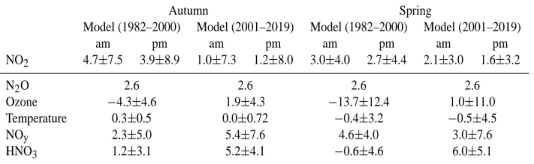
Table 2. Autumn and spring trends in NO2, N2O, ozone, temperature, NOyand HNO3derived from model results for Arrival Heights for
the periods 1982–2000 and 2001–2019. Trends are given in % per decade (temperature trends are shown in K/decade). The quoted errors are ±2σ .
Autumn Spring
Model (1982–2000) Model (2001–2019) Model (1982–2000) Model (2001–2019)
am pm am pm am pm am pm NO2 4.7±7.5 3.9±8.9 1.0±7.3 1.2±8.0 3.0±4.0 2.7±4.4 2.1±3.0 1.6±3.2 N2O 2.6 2.6 2.6 2.6 Ozone −4.3±4.6 1.9±4.3 −13.7±12.4 1.0±11.0 Temperature 0.3±0.5 0.0±0.72 −0.4±3.2 −0.5±4.5 NOy 2.3±5.0 5.4±7.6 4.6±4.0 3.0±7.6 HNO3 1.2±3.1 5.2±4.1 −0.6±4.6 6.0±5.1
cycle are reproduced by the model. Systematic underpredic-tion of the measurements by the model is most likely due to
an underprediction of the amount of NOy. Although this
af-fects the absolute values of the NO2slant columns, the
per-centage trends from the model are not directly affected by
any mis-specification of the NOyamounts.
Modeled and measured linear trends for the period 1980– 2000 agree within the 2σ uncertainty range, for both the sun-rise and sunset cases. Both the model and measurements
show a greater rate of increase of NO2compared with N2O
suggesting a change in the partitioning of the oxides of
ni-trogen over Lauder. Model NOyand HNO3trends over the
same period confirm that, in the model, there is a change in
partitioning of the NOy family from the reservoir HNO3 to
the more chemically active NOxspecies.
The largest discrepancy between modeled and measured
NO2trends occurs in springtime when model NO2trends are
lower than the trends derived from measurements for both sunrise and sunset cases. The annually varying trends still agree at the 2σ level. It is not clear at this time what is
caus-ing the model to underpredict the NO2trends during this time
of the year. Polar vortex air mixing into mid-latitudes does not occur until early summer which rules out vortex air being the cause. Failure of the model to capture changes in chem-istry or dynamics or both could explain the discrepancy in
NO2trends.
Significant changes in the rate of increase of NO2 (at a
SZA of 90◦) are predicted by the model for the period 2001–
2019 compared with the period 1980–2000. Trends in NO2
are greater than the trends in N2O (and NOy) for the
pe-riod 1980–2000 with a reverse for the pepe-riod 2001–2019.
Changes in the NO2 trends are associated with changes in
HNO3trends, the ratios NOx/NOyand HNO3/NOybeing
an-ticorrelated.
Concurrent changes in ozone and stratospheric halogen trends are also found in the model results when compar-ing the 1980–2000 period with 2001–2019 but without addi-tional sensitivity experiments it is not possible to fully
deter-mine the nature of the coupling between the NOypartitioning
and other variables within the model.
7.2 Arrival Heights
As was the case with the Lauder comparison, the model re-sults at Arrival Heights reproduce well the measured
sea-sonal and diurnal cycles of NO2 slant column densities at
sunrise and sunset. Autumn model results consistently un-derestimate the measured values. The most likely reason for
this is an underestimation of the amount of NOyin the model
during this season.
Large variability in both the measured and modeled slant column densities result in large estimates in the errors of the
trends in NO2, ozone and temperature relative to the trends
themselves. This makes interpretation of the trend results difficult and care must be taken in assigning significance to the conclusions drawn.
Autumn trend results for Arrival Heights are similar to the
annually averaged results from Lauder. NO2increases at a
faster rate than N2O (and NOyin the model) for the period
1980–2000, followed by a decrease in the NO2trends for the
2001–2019 period. Modeled HNO3indicates that the
parti-tioning of NOyfollows a similar course to the Lauder results
with an increase in the relative amount of NOxat the expense
of HNO3up to approximately the year 2000. This change is
reversed in the model for the period 2001–2019.
For the chemically and dynamically active Antarctic
spring, secular changes in NOy partitioning are less
pro-nounced. NO2, HNO3and N2O (NOy) trends are all
simi-lar over the whole period of the integration. Denitrification of the polar stratosphere is an important process which oc-curs during the winter/spring period and is expected to sig-nificantly influence the trends in the oxides of nitrogen over Arrival Heights during spring. Currently the model uses a simple NAT/ice sedimentation scheme using a fixed sedi-mentation velocity as thus are not expected to capture the full detail of this process.
Results from both Lauder and Arrival Heights demonstrate
that changes in NO2 slant column densities derived from
UMETRAC output follow the observed trends for the period 1981–2000. This suggests processes influencing the nitrogen chemistry within the model are reasonably well represented.
Interestingly, the model prediction of the trends in NO2and
HNO3for the period 2001–2019 show a reversal compared
with the period 1981–2000. NO2trends are predicted to fall
below the N2O trends, associated with an increase in the
HNO3 trends indicating a shift in the partitioning of NOy
away from it’s active form at Lauder and Arrival Heights (au-tumn) over the coming two decades. Additional analysis of the model data is required to examine to what fraction of the
change in NO2and HNO3trends can be attributed to
circu-lation changes and what fraction is associated with chemical forcing.
Acknowledgements. The authors would like to thank G. Keys for his work on the reanalysis of Arrival Heights measurements. The NO2measurements used in this publication were obtained as part
of the Network for Detection of Stratospheric Change (NDSC) and is publicly available (see http://www.ndsc.ncep.noaa.gov). This work was funded by the New Zealand Foundation of Research Science and Technology.
Edited by: J. Brandt
References
Ajtic, J., Connor, B., Lawerence, B., Bodeker, G., Hoppel, K., Rosenfield, J., and Heuff, D.: Dilution of the Antarctic ozone hole into southern midlatitudes: 1998–2000, J. Geophys. Res., accepted, 2004.
Austin, J.: On the explicit versus family solution of the fully diurnal photochemical equations of the stratosphere, J. Geophys. Res., 96, 12 941–12 974, 1991.
Austin, J. and Butchart, N.: Coupled chemistry-climate model sim-ulations for the period 1980–2020: Ozone depletion and the start of the ozone recovery, Q. J. R. Meteorol. Soc., 129, 3225–3249, 2003.
Bodeker, G., Boyd, I., and Matthews, W.: Trends and variability in vertical ozone and temperature profiles measured by ozoneson-des as Lauder, New Zealand: 1986-1996, J. Geophys. Res., 103, 28 661–28 681, 1998.
Bodeker, G., Scott, J., Kreher, K., and McKenzie, R.: Global ozone trends in potential vorticity coordinates using TOMS and GOME intercompared against the Dobson network: 1978–1998, J. Geo-phys. Res., 106, 23 029–23 042, 2001.
Brasseur, G. and Solomon, S.: Aeronomy of the middle atmosphere, D. Reidel Publishing Company, Dordrecht, The Netherlands, 2nd Edn., 1986.
Bucholtz, A.: Rayleigh-scattering calculations for the terrestrial at-mosphere, Appl. Opt., 34, 2765–2773, 1995.
Crutzen, P.: The influence of nitrogen oxides on the atmospheric ozone content, Q. J. R. Meteorol. Soc., 96, 320–325, 1970. Cullen, M. and Davies, T.: Conservative split-explicit integration
scheme with fourth-order horizontal advection, Q. J. R. Meteo-rol. Soc., 117, 993–1002, 1991.
DeMore, W., Sander, S., Golden, D., Hampson, R., Kurylo, M., Howard, C., Ravishankara, A., Kolb, D., and Molina, M.: Chem-ical kinetics and photochemChem-ical data for use in stratospheric mod-elling, Tech. Rep. Evaluation number 12, Pasadena, Ca, 1997. Fish, D., Roscoe, H., and Johnston, P.: Possible causes of
strato-spheric NO2trends observed at Lauder, New Zealand, Geophys.
Res. Lett., 27, 3313–3316, 2000.
Grainger, J. and Ring, J.: Lunar luminescence and solar radiation, Space Res., 3, 989, 1963.
IPCC: IPCC, Climate Change 2001: The Scientific Basis, Contribu-tion of Working Group 1 to the Third Assessment Report of the Intergovernmental Panel on Climate Change, Tech. rep., Cam-bridge, UK, 2001.
Johnston, P. and McKenzie, R.: NO2observations at 45◦S during
the decreasing phase of solar cycle 21, from 1980 to 1987, J. Geophys. Res., 94, 3473–3486, 1989.
Kalnay, E., Kanamitsu, M., Kistler, R., Collins, W., Deaven, D., Gandin, L., Iredell, M., Saha, S., White, G., Woollen, J., Zhu, Y., Leetmaa, A., Reynolds, R., M.Chelliah, Ebisuzaki, W., Higgins, W., Janowiak, J., Mo, K. C., Ropelewski, C., Wang, J., Jenne, R., and Joseph, D.: The NCEP/NCAR 40-year reanalysis project, Bull. Am. Meteorol. Soc., 77, 437–471, 1996.
Keys, J. and Johnston, P.: Stratospheric NO2 and O3 in
Antarc-tica: Dynamic and chemically controlled variations, Geophys. Res. Lett., 13, 1260–1263, 1986.
Keys, J. and Johnston, P.: Stratospheric NO2column measurements for three Antarctic sites, Geophys. Res. Lett., 15, 898–900, 1988. Liley, J., Johnston, P., McKenzie, R., Thomas, A., and Boyd, I.: Stratospheric NO2variations from a long time series at Lauder,
New Zealand, J. Geophys. Res., 105, 11 633–11 640, 2000. McKenzie, R. and Johnston, P.: Springtime stratospheric NO2in
Antarctica, Geophys. Res. Lett., 11, 73–75, 1984.
McKenzie, R., Johnston, P., McElroy, C., Kerr, J., and Solomon, S.: Altitude distributions of stratospheric constitutuents from ground-based measurements at twilight, J. Geophys. Res., 96, 15 499–15 511, 1991.
McLinden, C., Olsen, S., Prather, M., and Liley, J. B.: Understand-ing trends in stratospheric NOyand NO2, J. Geophys. Res., 106,
27 787–27 793, 2001.
Minschwener, K., Salawitch, R., and McElroy, M.: Absorption of solar radiation by O2: Implications for O3and lifetimes of N2O,
CFCl3and CF2Cl2, J. Geophys. Res., 98, 10 543–10 561, 1993. Plumb, R. and Ko., M. K. W.: Interrelationships between mixing
ratios of long-lived stratospheric constituents, J. Geophys. Res., 99, 10 145–10 156, 1992.
Randel, W., Wu, F., Oltmans, S., Rosenlof, K., and Nedoluha, G.: Interannual cahnges in stratospheric water vapour and correla-tions with tropical tropopause temperatures, J. Atmos. Sci., 61, 2 133–2 148, 2004.
Randeniya, L., Vohralik, P., Plumb., I., and Ryan, K. R.: Heteroge-neous BrONO2hydrolysis: Effect on NO2columns and ozone at high latitudes in summer, J. Geophys. Res., 102, 23 543–23 557, 1997.
Randeniya, L., Vohralik, P., and Plumb, I.: Stratospheric ozone depletion at northern mid latitudes in the 21st cen-tury: The importance of future concentrations of greenhouse gases nitrous oxide and methane, Geophys. Res. Lett., 29, doi:10.1029/2001GL014 295, 2002.
Rinsland, C., Weisenstein, D., Ko, M. K. W., Scott, C., Chiou, L., Mahein, E., Zander, R., and Demoulin, P.: Post-Mount Pinatubo eruption ground-based measurements of HNO3, NO and NO2 and their comparison with model calculations, J. Geophys. Res., 108, doi:10.1029/2002JD002 965, 2003.
Rodriguez, J., Ko, M. K. W., and Sze, N.-D.: Role of heterogeneous conversion of N2O5on sulphate aerosols in global ozone losses,
Nature, 352, 134–137, 1991.
Rosenlof, K., Oltmans, S., Kley, D., Russell, J., Chiou, E.-W., Chu, W., Johnson, D., Kelly, K., Michelsen, H., Nedoluha, G., Rems-berg, E., Toon, G., and McCormick, M.: Stratospheric water vapour increases over the past half-century, Geophys. Res. Lett., 28, 1195–1198, 2001.
Sander, S., Ravishankara, A., Friedl, R., DeMore, W., Golden, D., Kolb, C., Kurylo, M., Molina, M., Hampson, R., Huie, R., and Moortgat, G.: Chemical kinetics and photochemical data for use in stratospheric modelling, Tech. Rep. Evaluation number 12: Update of key reactions, Pasadena, Ca, 2000.
Scaife, A., Butchart, N., Warner, C., Stainforth, D., Norton, W., and Austin, J.: Realistic quasi-biennial oscillations in a simulation of the global climate, Geophys. Res. Lett., 27, 3481–3484, 2000. Schofield, R., Connor, B. J., Kreher, K., Johnston, P., and Rodgers,
C.: The retrieval of profile and chemical information from ground-based UV-Visible spectroscopic measurements, J. Quan-titative Spectroscopy and Radiative Transfer, 86, 115–131, 2003.
Solomon, S., Schmeltekopf, A., and Saunders, R.: On the interpre-tation of zenith sky absorption measurements, J. Geophys. Res., 92, 8311–8319, 1987.
SPARC: 2000: SPARC assessment of upper tropospheric and strato-spheric water vapour, Tech. Rep. WMO-TD No. 1043, WCRP Series Report No. 113, SPARC Report No. 2, Berrieres le Buis-son Cedex, http://www.aero.jussieu.fr/∼sparc/WAVASFINAL
000206/WWW wavas/WavasComplet.pdf, 2000.
Warner, C. and McIntyre, M.: Toward an ultra simple spectral grav-ity wave parameterization for general circulation models, Earth Planets Space, 51, 475–484, 1999.
WMO: Scientific Assessment of Ozone Depletion: 1991, WMO Global Ozone Research and Monitoring Project, Tech. Rep. Re-port No. 25, Geneva, Switzerland, 1991.
WMO: Scientific Assessment of Ozone Depletion: 1998, WMO Global Ozone Research and Monitoring Project, Tech. Rep. Re-port No. 44, Geneva, Switzerland, 1999.
WMO: Scientific Assessment of Ozone Depletion: 2002, WMO Global Ozone Research and Monitoring Project, Tech. Rep. Re-port No. 47, Geneva, Switzerland, 2003.
Zander, R., Ehhalt, D., Rinsland, C., Schmidt, U., Mahieu, E., Rudolph, J., Demoulin, P., Roland, G., Delbouille, L., and Sauval, A.: Secular trend and seasonal variability of the column abundance of N2O above the Jungfraujoch station determined