Separation of multiple echoes using a high-resolution spectral analysis for SuperDARN HF radars

HAL Id: insu-02183268

https://hal-insu.archives-ouvertes.fr/insu-02183268

Submitted on 15 Jul 2019

HAL is a multi-disciplinary open access

archive for the deposit and dissemination of

sci-entific research documents, whether they are

pub-lished or not. The documents may come from

teaching and research institutions in France or

abroad, or from public or private research centers.

L’archive ouverte pluridisciplinaire HAL, est

destinée au dépôt et à la diffusion de documents

scientifiques de niveau recherche, publiés ou non,

émanant des établissements d’enseignement et de

recherche français ou étrangers, des laboratoires

publics ou privés.

Separation of multiple echoes using a high-resolution

spectral analysis for SuperDARN HF radars

Laurent Barthès, R. André, J.-C Cerisier, J.-P Villain

To cite this version:

Laurent Barthès, R. André, J.-C Cerisier, J.-P Villain. Separation of multiple echoes using a

high-resolution spectral analysis for SuperDARN HF radars. Radio Science, American Geophysical Union,

1998, 33 (4), pp.1005-1017. �10.1029/98RS00714�. �insu-02183268�

Radio Science, Volume 33, Number 4, Pages 1005-1017, July-August 1998

Separation of multiple echoes

using a high-resolution

spectral

analysis for SuperDARN HF radars

L. Barthes,

1 R. Andre,

2 J.-C. Cerisier,

1,3

and J.-P. Villain

Abstract. Data obtained with coherent HF backscatter radars of the Super Dual Auroral Radar

Network (SuperDARN) are routinely analyzed with a standard algorithm based upon the

simplifying assumption that the backscattered signal consists of a single source, characterized by

its Doppler velocity and spectral width. More complex situations are often encountered where the

signal includes several sources, either due to the additional existence of ground scatter or due to

multiple ionospheric lines, related to a strongly inhomogeneous velocity field. We analyze the

response of the standard algorithm to such signals and we propose to use high-resolution spectral

analysis methods, namely• the multiple signal classification (MUSIC) method, to separate

multiple echoes with different velocity and spectral width. We analyze theoretically the

autocorrelation function of the received signal, and we show that its structure satisfies the criteria

for processing by the MUSIC algorithm. A statistical numerical simulation of SuperDARN data

processing by the MUSIC method allows us to evaluate the performances and the limits Of

applicability of the method. We show and illustrate with examples taken from experimental data

that the main imprr3vements are (1) the correct sep'aration of mixed echoes from ground and

ionosphere, which enhances the quality of ionospheric convection measurements, and (2) the

capability to resol,ve multiple ionospheric sources which appear in regions of inhomogeneous

convection. These multiple sources can be used to resolve small-scale structures in the velocity

field.

1. Introduction

The Super Dual Auroral Radar Network

(SuperDARN) coherent HF radars have been designed to monitor the large-scale ionospheric convection

[Greenwald et al., 1995]. From the signal coherently

backscattered by electron density irregularities frozen in

the ionospheric plasma, the radial component of the

convection velocity can be deduced. Using two radars

situated at remote sites and sharing a common field of

view, a vector convection map can be obtained. The

transmitted signal consists in a multipulse sequence, a

•Centre d'Etude des Environnements Terrestre et Planttaires, UVSQ/CNRS, Saint-Maur-des-Fossts, France

2Laboratoire de Physique et Chimie de l'Environnement, CNRS,

Orltans, France

3Also at Universit6 Pierre et Marie Curie, Paris, France.

Copyright 1998 by the American Geophysical Union.

Paper number 98RS00714.

0048-6604/98/98RS-00714511.00

technique initially developed by Farley [1972] for

incoherent radars and successfully applied to HF radars

by Greenwald et al. [1985]. The Doppler velocity is derived from the complex autocorrelation function

(ACF) of the signal returned from the ionosphere. The

ACF generally fits a damped complex sine wave. The slope of the time variation of the phase gives the

Doppler velocity, and the spectral width is related to the

damping factor. Occasionally, the ACF is more

complex, as can be expected when several sources are

simultaneously present in the target. The most common

case is that of an ionospheric source superimposed to a

ground echo. Some cases also result from two

simultaneous ionospheric echoes produced by a velocity

shear present in a single radar cell. When interpreted as

a single damped sine wave, these complex ACFs lead

usually to erroneous values of the velocity and spectral

width. In this study, we focus our attention on these cases in order to separate the contribution of the

different sources to the ACF. Because of the small

number of points of the ACF (typically 17-20), the

frequency resolution of the Fourier transform method is

not sufficient. A high-resolution method is more

appropriate, namely, the multiple signal classification

(MUSIC) method described by Schmidt [ 1986].

The standard processing technique of the radar data,

which is valid in the case of a single source, will be

briefly reviewed in section 2. In section 3, we will

consider the case of two sources. The structure of the

ACF is investigated theoretically, and examples taken

from the SuperDARN radars will illustrate the

inadequacy of the standard method in that case. The

alternate method based on the MUSIC algorithm will be

described in section 4, and a statistical evaluation of its capability to provide correct results will be presented.

Finally, section 5 will discuss examples illustrating the

potential benefits of the high-resolution spectral

analysis for geophysical purposes.

2. The Standard Analysis

Before investigating the case of several sources, let

us recall the standard situation when a single source is

present and investigate how the standard method of

analysis works. We will first describe the multipulse

emission scheme and its processing to calculate the ACF. We will then present how the physical

parameters, velocity, and spectral width are extracted

by the standard method.

2.1. Multipulse and Autocorrelation Function

The main advantages of a multipulse system have

been thoroughly described by Farley [1972]. The basic

principle is to transmit a sequence of pulses such that

the time delays between any two pulses of the sequence

are different and form a regular series, thus allowing us

to calculate the corresponding delays of the ACF. The

pulse length defines the range resolution or,

equivalently, the radial length of the elementary cell in

the radar field of view. One of the multipulse schemes currently used by the SuperDARN radars is shown in Figure 1. The basic scheme has evolved slightly with

time, but the main characteristics remain similar to

those used in this study. The pulse length is 300 Hs, giving a resolution of 45 km in range. The time separation between pulses is an integer multiple of

•--2.4ms. When receiving, the radar signal is

digitized with a sampling period of 300 Hs, equal to the

pulse length. From the seven-pulse sequence, 17 delays

of the ACF are calculated. The total signal received at a

given time is the sum of the signals backscattered from

17-r• 2.4 msec ß 1 121' e 13'r o = 1 lra ß 10Ta, ß ß 9Ta ß : 2To: 0 10 20 30 40 50 60 Time (msec)

Figure 1. Example of a seven-lag multipulse scheme used by

the Super Dual Auroral Radar Network (SuperDARN) radars. This sequence allows determining 17 points of the

autocorrelation (ACF) function of the backscattered signal.

different ranges and corresponding to the pulses

previously transmitted. For instance, 33 ms after the

start of the pulse sequence, the received signal will be

the sum of the echoes backscattered at ranges 1710 km

(from the second pulse of the sequence) and 630 km

(from the third pulse). The echo backscattered from the

range 4950 km (first pulse) can be neglected, because

echoes returning from ranges over 3500 km are usually

too faint. The received signal can be written:

S 0 = .,•1

e-JrøItø

+ A2e-Ja'2tøe

-j'•2

(1)

where t o is the time of the measurement, here 33 ms; to 1

and ro 2 are the angular frequencies of the signals

backscattered from ranges 1710 ,and 630km,

respectively; and A l and -//2 are the associated

amplitudes. The phase ½2 is the phase difference

between the two signals. In order to calculate the ACF

for the range 1710 km and for the delay r (for instance,

r = 3 r0), we use also the signal received at time t o + r

(here 40.2 ms):

BARTHES ET AL.: SUPERDARN HIGH-RESOLUTION SPECTRAL ANALYSIS 1007

This signal is also the sum of two echoes, one from the

range 1710 km with the amplitude A' 1 (which can be

different from A 1 because of the time variation of the

scattering fluctuations), and one from the unwanted

range

2790 km (index

3). The product

S•S r is then

, ,* /a)l r

SoS r - A 1A 1 e' +

,*

A2A

1 e•(•-•ø2)Oe•'lre

•e2

+

,

A1A3

e• 603-•0•

)0

e2•O3•e•e3

+

,

A2

A3

e • (•o3-•o2)o

e •o3•

e • (•3-•2)

(3)

This relation is valid for a single multipulse sequence.

Only the first term in the right-hand side of (3)

represents the ACF for the range 1710 km and the delay

3r 0. The three remaining terms are cross products between different ranges. Their relative amplitude is

reduced by repeating the multipulse scheme. The phases

69 i are random variables, due to the incoherence of the

phase of the fluctuations which are responsible for the

backscatter, at times separated by the delay between

successive multipulse sequences, typically 100 ms. The

damping

of these

terms

is proportional

to N 1/2,

where

N

is the number of multipulse sequences. A relative

damping of 8.6 is obtained when the ACF is averaged

over 75 multipulses. From here on, only the first term in

(3) will be considered

C(r ) = SoS • = A, A• e (4)

This technique allows us to obtain 17 points of the

complex ACF in each of the 70 range gates, every 7 s.

2.2. Obtaining Velocity and Spectral Width

From the ACF

The standard method for obtaining the Doppler

velocity and the spectral width has been described by

Villain et al. [1987]. The velocity is derived from the

Doppler frequency, deduced from the phase of the ACF

by a linear least squares fit. The phase ½ is given by

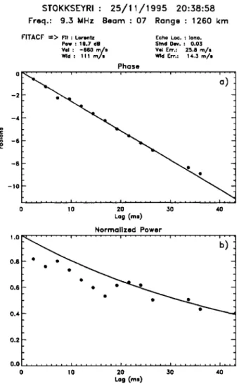
q•--arctan(I/R), where R and I are the real and imaginary parts of the ACF. A typical example taken from the Stokkseyri SuperDARN radar is given in

Figure 2a. Dots represent the experimental values of the

phase, and the solid line is the least squares fit to these

points. In this example, the cross terms in (3) have no

influence on the experimental ACF, as expected, thanks

to the averaging process. The relation between the

Doppler frequency to and the velocity v is

STOKKSEYRI : 25/11/1995 20:58:58 Freq.: 9.3 MHz Beam : 07 Range : 1260 km

FITACF => nt: Lorentz Echo Loc. :Iono. Pow: 19.7 da $tnd Der. : 0.03

Vel : -660 m/s Vel Err.: 25.8 m/s Wld : 111 m/s Wld Err.: 14.3 m/s Phase -10 ... i ... i ... i ... I , , 0 10 20 30 40 Lag (ms) Normalized Power 0.8

•-_

' ' . .

.•

ß

Figure 2. Illustration of the "standard" analysis of the SuperDARN ACFs. (a) The Doppler frequency is determined by a linear least squares fit of the phase of the ACF. (b) The spectral width is deduced from the fit of the power to a

Gaussian or a Lorentzian spectrum.

c

v - ••o (5)

2(.O e

where c is the velocity of light and toe is the transmitter

frequency. In the above example, the Doppler velocity

is -660 m/s. The estimated velocity error remains small,

less than 30 m/s.

The spectral width is deduced from the time variation

of the power

P(r) of the ACF [P = (R

2 + 12)

•/2]. Two

types of fits are performed, one by an exponential profile (Lorentzian spectrum) and one by a Gaussian

profile (Gaussian spectrum). These are least squares fits

The better of the two fits in the least squares sense gives

the selected spectral width. The physical meaning of

these two models for the shape of the spectrum is

discussed below. Figure 2b shows an example of a

Lorentzian fit. The relation between the damping factor

a and the spectral width w of the Lorentzian spectrum is

c

w - 2a (6)

209 e

In the above example, the spectral width is 111 m/s.

The estimated error is less than 15 m/s.

Previous statistical studies [Villain et al., 1987] have shown that about 80% of the ACFs are best fitted by a

Lorentzian spectrum. The physical interpretation of

these different behaviors is related to the ratio of the

correlation length to the radar wavelength. The theory

shows that Lorentzian spectra occur when this ratio is

larger than unity. Villain et al. [1996] have shown that

the correlation length is typically 1 m, thus confirming

the small value of the above ratio and the observed

predominance

of Lorentzian

spectra.

Hanuise et al.

[ 1993] have introduced a mixed type of damping of the

ACF: Gaussian for short delays and Lorentzian for long

delays.

3. The Case of Two Sources

The case where two sources are simultaneously

present at the same range will now be considered.

Owing to propagation conditions, this happens when a

ground echo, characterized by a very small Doppler

velocity and a narrow spectral width, is present together

with an ionospheric echo. From here on, only the

averaged form of the ACF, as given by (4), will be

considered. Neglecting the damping of the signal, the

ACF in the case of two sources can be written

C (•') - (•412

q-

,B)e

s•"•

+ (A22

+ )e

s•'2• (7)

with

fl - A1A

2 e • (•,,-•,2)o

e- •½

(8)

Here tOl and to2 are the frequencies of the two sources;

A 1 and

A 2 are their respective

real amplitudes;

and 6)is

their phase difference. Relation (7) shows that the ACF

is now given by the sum of the ACFs of each source, with an additional coupling term. Again, and for the

same reasons as for the coupling term between different

ranges which appeared in equation (3), this term

vanishes with the averaging procedure.

Up to now, the damping of the ACF has been

neglected. It can be reintroduced through a velocity

(frequency) spread around co. This spread will cause a

damping of all the terms of the ACF. For a Lorentzian

damping, the ACF can be written

C (r) = A•2e

-'•'•e

• + A22e

-'•2•e

•¾

(9)

From this relation, it is clear that the time variation of

the phase of the ACF is no longer linear. Figure 3a

shows the variation of the phase for the case of two

sources,

a ground

echo (A1--0.7, V 1 = 0, a 1 = 0) and

an ionospheric source (A 2 = 1, V 2 = 200 m/s,

a 2 = 150 m/s).

The phase

oscillates

around

zero,

and

it

is clear from the figure that the standard method is not

appropriate. It is important to notice that the linear least

squares fit of the phase leads to a small value of the

velocity (11 m/s in the present example), thus

suggesting that the standard method is able to detect the

ground echo. However, the determination of the

spectral width is completely erroneous (166 m/s instead

of 0 m/s). This is extremely important because the usual

criteria for identifying ground echoes are based on their

physical characteristics, namely, a small velocity

associated to a narrow spectral width. The present

simulation is typical of a false identification of an

ionospheric echo with a small velocity, whereas the

ACF represents an ionospheric velocity of 150 m/s

superimposed to a ground echo. Let us remark,

however, that the above confusion can be detected by a

careful analysis of the quality of the fits of the phase

and amplitude.

In Figure 3b, representing experimental data, a

behavior similar to the simulation of Figure 3a is observed. The linear fit leads to an almost horizontal

slope on which an oscillation is superimposed. The

small value of the slope is indicative of a small velocity

which can be related to a ground echo, while the faster

oscillation is indicative of an ionospheric source having

a velocity of the same order as in the simulation of

Figure 3a. Figure 3c is a second experimental example

where now the larger slope of the fit indicates a larger

velocity. This large slope, together with the

superimposed oscillation, suggests the presence of two

ionospheric sources.

4. The High-Resolution MUSIC Method

In the case of short data sequences, the Fourier

transform technique provides poor spectral resolution.

BARTHES ET AL.: SUPERDARN HIGH-RESOLUTION SPECTRAL ANALYSIS 1009

Simulafad ACF' wlth two components M

...

c

,Y_., TM

1.0• ß ß

i=l

-1.0

1 First

Component:

A

= 1.01

V

--

750

m/s

w

= 100

m/s

-1,5• ... i ... i ... , ... o Lag (ms) •- 0.5 ... O J3 g -o.s

$tokkseyrl : 25/11/1995 20:04:29 Range: 1620 km Freq.: 9.4 MHz

ß œ ß .

_1.01

ß

Stokkseyrl : 02/09/1995 09:12:21 Range: 1710 km Freq.: 12..3 MHz , , , . . .

0 ß ß _

, , , , , , . . . , ... i ... i ...

o 1 o 20 30 40

Log (ms)

Figure 3. Phase (dots) of the ACF when two sources are simultaneously present in the backscattered signal. (a)

Simulated ACF with ground and ionospheric echoes. (b)

Experimental ACF with ground and ionospheric echoes. (c) Experimental ACF with two ionospheric echoes. The solid line represents the fit of the phase by the standard (single source)

method.

appeared which are designed to enhance the spectral

resolution. They are all based on a priori hypotheses on

the structure of the signal. Among them, the multiple

signal classification (MUSIC) method, described by

Schmidt [1986], assumes a signal composed of a sum of

complex sine waves with additional white noise. The

structure of the ACF given by (9) suggests that this

method is appropriate to the SuperDARN data.

4.1. Summary of the MUSIC Method

Let us now write the ACF as a sum of M damped

sine waves.

with

(lO)

z, - e -a'+•a" (11 )

Let Y n be the vector built with p

observations organized in reverse order'

consecutive

Y. = [Cn,

Cn_l,...,Cn.p+l]

T

(12)

The pxp autocorrelation

matrix Rp is defined

as the

expectation

of YnYn

+, where

the

plus

sign

denotes

the

transpose of the complex conjugate. In the presence of

damping, the matrix cannot be calculated by the usual

method using both direct and reverse order in the C n

series that constitute the Yn vector. The matrix is simply

calculated as

=

=•

Y.Y,:

(13)

R•, E 'Y" N- p +

1

,=•,_,

where E( ) is the mathematical expectation operator and N is the length of the data record (the number of

points in the ACF). It can be shown that if C n is given

by (10) and if Rp is estimated

with the above

equation

(13), the rank of Rp is equal

to M, which

means

that

only Meigenvalues/l i, i•[1,p], are nonzero values. The

M eigenvectors Vi associated with these eigenvalues

span the signal subspace. The signal has only projection

in this subspace'

M

R•, - E A/V/V/+

(14)

The other eigenvectors

(¾•.;..¾;,)

define the noise

subspace (only the noise has projection in this

subspace). Owing to the properties of the

autocorrelation matrix, these two vector subspaces are

1

1]T

orthogonal.

Let Z--[zø,z

...

z

p-

be a vector

belonging to the signal subspace. The scalar product

between this vector and each of the noise vectors is

equal to zero. This property is used to derive the

polynom.of MUSIC:

2

z+v,i

-z+. .v,v/.z_-z+.Q.z

(15)

i=M+I i=M+I

The roots of this polynom z i give through relation (11)

M signals are associated to the M roots which are

closest to the unit circle in the z space. '7' 400

When white noise is present, it can be shown

[Marpie, 1987] that the eigenvalues of the noisy •_ 200

o

autocorrelation matrix are equal to those of the

nonnoisy

matrix

plus

the noise

variance.

The method •

0

remains the same. When M is unknown, the respective o

dimensions of the signal space and noise space are _{> -200}

determined from the analysis of the sequence, in c

decreasing

order, of the eigenvalues:

The signal •-400

eigenvalues constitute a decreasing series, whereas the 0

noise eigenvalues are all equal and below the smallest

signal eigenvalue. A noise power estimation is thus available. From this value and from the noisy autocorrelation matrix it is easy to get the unnoisy

autocorrelation matrix and to derive the power or the _4O0

signal-to-noise ratio (SNR) of each damped sine wave.

4.2. Principle of the Simulation

In order to test the capability of the MUSIC method to derive SuperDARN physical parameters, a large

number of simulated ACF have been analyzed. The

velocity and the spectral width of the solutions have been systematically calculated. The total number of points in the ACFs is 20, among which are three missing values (lags 6, 7, and 14) called "bad lags,"

which also occur in the real data, due to interruptions of

reception during transmission periods or other

perturbations. The dimension of the autocorrelation

matrix is chosen to be p--8, which represents a good

compromise between the maximum number of sources

expected in the signal and the number of points in the ACF. The result of the analysis of each ACF has been attributed one of three possible labels: (1) correct

determination (if the velocity is within 50 m/s of the

nominal value); (2) false determination (if the velocity

is not within 50 m/s of the nominal value); and (3) no

determination (if the algorithm identifies only noise, no

signal solution being determined).

4.3. Single Source

An initial test of the MUSIC algorithm has been

performed in the simplest case when the signal consists

of a single source. The spectral width has been varied from 0 to 800 m/s by steps of 25 m/s. In each case, the velocity has been varied from-800 m/s to +800 m/s,

with a step of 100 m/s. A series of 750 samples have

been examined for each velocity and spectral width,

with a uniform distribution of the signal-to-noise ratio

between 3 and 20 dB. Figure 4 shows the results of the

(A) Lorentzian

Spectrum

200 400 600 800 Spectral width (m/s) o 200 -200 -4OO o

(B) Lorentzi(]n Spectrum

(C) Lorentzi(:n

Spectrum

Figure 4. Statistical results of the simulation of the analysis of

the SuperDARN ACFs with the multiple signal classification (MUSIC) algorithm. (a) Mean error (solid line) and variance (dotted line) in the velocity determination. (b) Mean error (solid line) and variance (dotted line) in the spectral width determination. (c) Probabilities of different results of the MUSIC analysis (correct, false, or no velocity determination). The ACF comprises one single source with a Lorentzian

BARTHES ET AL.' SUPERDARN HIGH-RESOLUTION SPECTRAL ANALYSIS 1011

analysis for the case of an exponential decay

(Lorentzian spectrum). Figure 4a represents the mean

(over velocity and SNR) velocity error as a function of

the spectral width. This mean error (solid line) in the

velocity determination is zero, which means that the

velocity determination remains unbiased, whatever the

spectral width. Of course, the standard deviation of the

error (dotted lines) increases with spectral width but

remains always below the half of the spectral width. It

must be observed that when the spectral width is large,

the amplitude of the ACF decreases very rapidly and

the data for large delays are strongly corrupted by

noise, leading to a poor (or impossible) estimate of the

parameters of the source. The mean error in the spectral

width shown in Figure 4b indicates that the spectral width is slightly overestimated for widths below

500 m/s and underestimated beyond. The bias on the

determination of the spectral width can be explained as

follows: The roots of the MUSIC polynom associated to

the signal are identified by their proximity to the unit

circle (Izil--1). For large spectral widths, the root

moves away from the unit circle and can be confused

with roots associated to noise. So only the roots with an

underestimated spectral width are close enough to the

unit circle to be considered as representing the signal,

whereas overestimated values are considered as

belonging to the noise subspace and thus rejected.

Figure 4c shows estimates of the probability of a correct

estimation of the velocity, the probability of an incorrect determination of the velocity, and the probability that the source is not detected. For small

spectral width the probability of a correct detection is

very good, whereas the probability of no or false

estimation remains negligible. The probability of a false

estimation reaches 5% when the spectral width is

250 m/s and 25% when the spectral width is 500 m/s.

The damping of ionospheric backscattered signals is not

necessarily exponential. Gaussian damping (leading to a

Gaussian spectrum) is sometimes observed, although

less often. Although the MUSIC algorithm is not designed for Gaussian damping (two or more close

sources can be obtained instead of a single source), the

method has been applied to such signals. Figure 5 shows the results of the simulation performed for

Gaussian spectra with all other conditions remaining the

same as for Figure 4. The main difference is that the probability of a false estimation now reaches only 3% for a spectral width of 250 m/s and raises to 30% for 500 m/s. The probability of no estimation is not

different in both cases.

At this point, it is necessary to mention that in the real

data, spectral widths larger than 500 m/s are relatively

inusual. However, from Figures 4 and 5 it is clear that

when such large spectral

widths are measured,

the

results

have

to be analyzed

with great

care.

The above simulations have been made with a minimum

3-dB threshold on the estimation of the SNR, whatever

the spectral

width.

Of course,

the probability

of a false

estimation

increases

with decreasing

SNR but also

with

-'-'- 400 F 2O0 o o o > -200 • -400 0

(A) Gaussian

Spectrum

ooo ! I i • i I i 200 400 600 Spectral width (m/s) 800 400 200 -200 -400 o

(B) Gaussian Spectrum

(C) Gaussian

Spectrum

0.0 ... '

increasing spectral width. If an upper limit (typically

5%) is set to the probability of a false estimation, a 1.0

variable SNR threshold has to be used, depending upon _0.8

the spectral width, a larger value of the threshold being

used for larger spectral widths. An analysis of the ._ _{- 0.6}

results of the simulation has led to define an

exponential

law:

SNRthreshoid(dB ) = 4.5 X exp(w/450.) (16) _(3.2

which limits the increase in the probability of error to _0.(3

less

than

5% for large

spectral

widths.

The

above

rule,

however, is difficult to apply directly because the SNR

can be overestimated by MUSIC. This happens when a

root of the MUSIC polynom belonging to noise is

attributed to a source, thus underestimating the noise 1.0

level. To avoid this problem, a minimum value of the

power for a root of the polynom to be considered as •.8

representing a source has been introduced. These two

thresholds (minimum SNR and minimum power) have

been systematically used in the simulations described

o 0.4-

below for the case of two sources. 4.4. ACF Comprising Two Sources

We now consider the case where two sources are

present in the ACF signal. In order to simulate best the

most common case of a ground-scattered echo

superimposed on an ionospheric echo, one of the

simulated signals is characterized by a zero velocity and

no damping (zero spectral width). The distribution of the ionospheric sources is similar to the "single source"

case presented above with regard to the velocity and

spectral width. Both signals have identical amplitudes.

Only the case of a Lorentzian spectrum will be

discussed here. Two cases must be considered

according to whether the velocity difference between

the two sources is larger or smaller than the resolution

of a Fourier analysis of the ACF (typically 250 m/s). The results are presented in Figure 6, in terms of probabilities, similar to those of Figures 4c and 5c.

When the velocities of the ionospheric and ground

echoes have a separation larger than the resolution of a

fast Fourier transform (FFT) analysis, the probability of

a correct identification of the two sources is the same as

for the single source case (Figure 6a). In other words,

the estimation of one source does not depend upon the

other. This can be demonstrated theoretically from the

Cramer Rao boundary [Delhote, 1985]. Figure 6a also

shows the effect of a SNR threshold. The probability of

a false determination is maintained below 5%, whatever the spectral width. The counterpart is a lower

Lorentzian Spectrum

•,

,' . .... No

estimate

200 40O 6OO 8OO

Spectral width (m/s) 0.2

Lorentzian Spectrum

Figure 6. Statistical results of the MUSIC analysis when two sources (ionospheric and ground) are present in the signal. The probabilities of different results (correct, false, or no velocity determination) for a Lorentzian ionospheric source are presented. (a) The source separation is larger than the resolution of the Fourier analysis. (b) The source separation is smaller than the resolution of the Fourier analysis.

probability of a correct estimate, typically 50% only for

a 300 m/s spectral width. The remaining 45% are

rejected by the threshold condition.

Figure 6b shows the results obtained when the

ionospheric and ground echoes have velocities too close

to be separated by FFF (AV < 250 m/s). The probability

of a correct estimation is considerably reduced, typically 60% at best. It must be noticed also that the

probability of a false estimation, although higher than in

the case of two well-separated sources, remains below

5%, whatever the spectral width.

Other simulations have been made for different

values of the relative amplitude of the two sources. It

can be shown theoretically that the variance of the

BARTHES ET AL.: SUPERDARN HIGH-RESOLUTION SPECTRAL ANALYSIS 1013

amplitude of the other [Delhote, 1985]. This was

confirmed by simulation with ground scatter amplitude

up to 30 dB above the ionospheric amplitude.

The simulations have also been analyzed to compare

the number of ionospheric sources given by MUSIC to

the real number. When only one ionospheric echo is

present, the probability of obtaining two or more

ionospheric echoes is less than 0.5% in the Lorentzian

case, whatever the spectral width, and between 0.5% and 1.5% (depending on the spectral width) in the

Gaussian case.

It must be kept in mind that all the above

probabilities have been obtained with the ACF of the

type defined in section 4.2. Other multipulse schemes can be designed which, by increasing the number of points in the ACF, are potentially able to improve the

quality of the results obtained with MUSIC.

5. Analysis of SuperDARN Data

With the MUSIC Algorithm

SuperDARN data have also been analyzed with the MUSIC algorithm. We present below examples which

confirm the capability of high-resolution methods to

resolve multiple sources in the scattered signal. We will

also illustrate the benefits, which can be obtained by the

use of MUSIC for the study of the ionospheric plasma

convection.

5.1. Ionospheric and Ground Echoes

Figure 7 shows Fourier spectra obtained from the

Stokkseyri radar in six adjoining cells (a 3x2 template

in range and beam). The data from the two beams are

separated by less than 2 min. In the beam-8 panels (left

column), the ground echo dominates the FFT spectrum.

The standard analysis (not shown in the figure) also detects the ground solution. In addition to the ground echoes, the MUSIC method detects two ionospheric

sources: one with a velocity of the order of-350 m/s

and one with a positive velocity between 500 and 750 m/s. In the beam-9 panels (right column), the dominant signal is due to the ionospheric negative velocity

source. This signal is clearly seen in the FFT spectrum

and confirmed by both the MUSIC and standard methods; MUSIC also detects a low velocity solution and the positive velocity ionospheric source. The

consistency of the MUSIC determinations in

independent cells argues strongly in favor of the

method.

Plate 1 shows an example of a SuperDARN radial velocity map. Plate l a displays the result of the standard analysis. It exhibits both ground echoes (in

grey) and ionospheric sources. Plates lb and lc display

the results of the MUSIC analysis for the same data set.

The most intense ionospheric source is shown in Plate

lb and the ground echoes in Plate l c. The comparison

of these three panels shows clearly that MUSIC

increases the spatial coverage of ionospheric sources to

regions where the standard method could identify only

ground echoes. This is particularly the case for the red-

orange area which is larger in Plate lb than in Plate 1 a; Comparison also shows that most of the ionospheric

echoes identified by the standard method are confirmed

by MUSIC. However, some echoes identified as "ionospheric" (green zone in Plate l a) by the standard

method become "ground" by the MUSIC analysis. This

means that the spectral width criterion used to distinguish between ground and ionospheric echoes

(w < 50 m/s) is, in fact, more severe with the standard

method than with MUSIC. It must be kept in mind that

although the choice of the above limit is based on the

analysis of a large number of data, it also contains

arbitrariness.

5.2. Ionospheric Sources: Comparison With ACF In order to evaluate the quality of the solution given by a processing algorithm, the ACF can be

reconstructed from that solution and compared with the

experimental ACF. Figure 8 shows the result of this

exercise for both the standard method and MUSIC, in a situation where MUSIC detects two ionospheric sources. Figures 8a and 8b display the real and

imaginary parts, respectively. For both components, the

MUSIC solution gives a much better fit to the experimental data than the standard analysis. The MUSIC solution in the above example is characterized

by two sources with velocities -805 m/s and -253 m/s.

The first of these velocities is not far from the value of

-711 m/s given by the standard method. This indicates

that again, like for the case of a ground echo, the

standard analysis can give an estimate of one of the two

velocities. However, and again also, the spectral width

given by the standard method is strongly overestimated

(1036 m/s against 211 m/s). The large spectral width

given by the standard method is the consequence of the

rapid decay of the ACF, due to the two-component

nature of the backscattered signal. It must be noted also

that the SNR in this example exceeds 10 dB, a large

lOO ,.• 80 • 60 100

• 8O

•' 20

SuperDARN Stokkseyri, 14: 25:25 Gate ' 56 Beam ß 8 ' ' ' ' ' ' ' ' ' I ... , i , , .... , , , I , , , , , , , , , Vel. MUSIC : , 4 m/s I :

-373

m/s .'

j

.

SuperDARN Stokkseyri, 14: 25:25 Gate ß 57 Beam ' 8

' ' ' ' ' ' ' ' ' i , , , , , , ' ' ' ' ' ' ' ' ' ' ' 8 Vel. MUSIC : 9 m/s -333 m/s •6 4 ß 2 ..-.. 8O •e 60 o o .>'_ - 2000 - 1000 0 1000 2000 Velocity (m/s)

SuperDARN Stokkseyri, 14: 2.5:2.5 Gate ß .58 Beam ß 8 ... I I ' ' ' ' ' ' ' ' Vel. MUSIC : -572 m/s

20

SuperDARN Stokkseyri, 14: 26:58 Gate ß 56 Beam ß 9 ' ' ' ' ... i ... I .... , .... i , , , , , , , , , Vel. MUSIC:

-3.54

m/s

. 56

m/s /

i

SuperDARN Stokkseyri, 14: 26:58 Gate ß 57 Be(]m ß 9

...

I ... Z''i .... •' .... I ...

-550 m/s / •A

:

- 10

mLs"/

I' •/• i

-

-2000 - 1000 0 1000 2000

Velocity

SuperDARN Stokkseyri, 14: 26:58 Gate ß 58 Beam ß 9

80 ... I ... I ... ! ...

Vel.

MUSIC:

-345 Ils

S4m/s

-2000 - 1 ooo o 1 ooo 2o00

Velocity

Figure 7. Comparison between the results of MUSIC and a fast Fourier transform (FF• analysis of the ACF in six adjoining cells. The multiple sources detected by MUSIC in the different cells are mutually consistent.

BARTHES ET AL.: SUPERDARN HIGH-RESOLUTION SPECTRAL ANALYSIS 1015 File - 94090214w ..- ;.:... ,, : Hour- 14:24:41 ...-'-'.... ß ," ., d ,

Radar-8

....--.':...

,:':i '":':"'"

... ' ...

.;.;:•

....

'"'

--

-" ' ... '

",,'

...

- 800-'

...

"

' ...

'

'

-- ' ...

600

Radar

8 -::';

."B .

200

...::

..

...

,:•

...

,-

- ...

.,:_

...

•,,.. :-: ...

',.,•

...

_ --

File

-94090214w

_..-'

":ø- "

_--:-:

_{.... -'}

' '"; ... : ... "'" "

_'

_'

'"

_:-

":"

_'-..

_{" -800}

Radar-

8 .-'C'

- ... .=,':

... ::...

'

-' .... •' - .... '"

'-

- 1000

' "'

•:-Velocity

..,::

;.•'::.

- , ..

.,.-

'?: ...

• .'%, :

'•

.>.,;

ß •.---•.

..

...

,-

- ...

. .... •,,: ... ; ... -,.:.•.-

•:'.

-•.

-.-:,- ...

. ...

Plate 1. Radial velocity maps obtained with the Stokkseyri SuperDARN radar, showing (a) the velocity

obtained with the standard analysis; (b) the ionospheric echoes detected by MUSIC; and (c) the ground

scatter echoes detected by MUSIC. The coordinates are geographic latitude and longitude.

performance of the standard method in terms of low SNR.

5.3. Application to a Convection Velocity Reversal

When a convection velocity reversal is present in the

radar field of view, multiple ionospheric sources are

expected to be observed in the range gates across which

the velocity shear occurs, whereas single sources are

expected on both sides of the shear. Figure 9 shows the

results obtained with the MUSIC algorithm, for the observation along a fixed direction of a steady shear over a 20-min period. Figure 9a shows the variation of

the mean (over the observation period) radial velocity

along the radar beam. The position of the shear is

clearly identified, with a homogeneous convection on

both sides. The probability of multiple sources shown in

Figure 9b is close to zero in the two regions of

homogeneous flow and shows a significant increase at

the location of the velocity shear. The SNR displayed in

Figure 9c also shows a maximum at the location of the

shear, suggesting that the shear is characterized by an

increased level of turbulence responsible for the

backscatter of the radar wave. The 10% maximum

probability of multiple sources in the shear indicates, however, that multiple ionospheric sources are not a highly common observation, despite favorable

conditions.

6. Conclusions

We have analyzed the limits of the standard method

used for processing SuperDARN HF radar data and

based upon the assumption of a single source in the

KAPUSKASING : 08/01/1996 18:50:50

Freq.: 11.5 MHz Beam : 08 Range : 2115 krn FITACF :> Fit: Lorentz Echo Loc.: Iono.

Paw: 10.4 dg Stnd Dev. : 0.23

Vel : -711 m/u Vel Err.: 68.8 m/u Wld : 1036 m/s Wld Err.: 327.1 m/u

MUSIC =>

I- Vel: -805 m/s -Wldth: 228.1 m/s - sa : 13.3 da 2- Vel : -253 m/s - Mdth : 364.9 m/u - SB : 12.0 dB

Real Parts

1.0•

Full

line-*

Experimental

data

Dashed line-" MUSIC method

L•

Dolled

line:

Standard

method

I'01

Full

line:

Experimental

data

.• 0,5;

Dotted

line:

Standard

method

,.=

-•

0,0

ß

...

-..

, ...-

...

• -0,5

0 10 20 30 443

lags (ms)

Figure 8. Comparison of the results of MUSIC and the

standard analysis with the experimental ACF. The MUSIC analysis gives a better fit to the experimental ACF, for both the (top) real and (bottom) imaginary parts.

ICELAND WEST File : 95090208w Mean Between 09:03:48 and 09:23:47 -- Beam : 12

600 L ... ' ... ' ... ' ... ' ... ' ... ,oo•- ø).

• 200

F

.• -200

"10

1

0 i ...

, ...

i ...

, ...

OI

... , ... , ... , ... , ... , ...

Figure 9. Analysis of a convection reversal with MUSIC. (a)

Radial velocity. (b) Probability of multiple ionospheric sources. (c) Signal to noise ratio. The shear is characterized by

an increased probability of multiple sources and an increased

SNR.

MUSIC high-resolution spectral analysis technique can

be used to handle more complex situations encountered

where the signal includes several sources, due either to

ground scatter or to multiple ionospheric lines. A

statistical numerical simulation of SuperDARN data

processed by the MUSIC method allows us to evaluate

the performances and limits of applicability of the

method. We also illustrate the capabilities of the

MUSIC method with examples taken from experimental

data.

We have shown that MUSIC is able to detect

ionospheric sources superimposed on a ground echo.

This capability depends strongly upon the spectral width; the larger the spectral width, the more difficult

the separation. We have also shown that MUSIC is able

to resolve multiple ionospheric sources, which are

present in regions of inhomogeneous convection. The

capability of MUSIC to separate several sources is a

complex function of the SNR, the spectral width of the

sources, and their separation. Low-velocity ionospheric

echoes are particularly difficult to separate from ground

scatter echoes.

Although no statistically significant evaluation has

yet been done, it is clear that measurements with

multiple sources are far from being the most common

situation in SuperDARN data. This means that the much

simpler and faster standard method of analysis, based

BARTHES ET AL.: SUPERDARN HIGH-RESOLUTION SPECTRAL ANALYSIS 1017

and powerful tool. However, the results of the present study can be used to better define the limits of

applicability of the standard method.

In further studies, the capability of MUSIC will be

evaluated for other multipulse schemes giving a larger

number of points in the ACF. The method will be also

used for several geophysical purposes: (1) to reevaluate

the physical interpretation of the spectral width in specific ionospheric regions; (2) to improve the accuracy of the localization of convection reversal

boundaries; (3) to detect small-scale structures; and (4)

to extend the field of ionospheric scatter to regions

screened by ground scatter.

Acknowledgements. The Kapuskasing SuperDARN radar

is operated by the Johns Hopkins University / Applied Physics Laboratory in the United States. The Stokkseyri SuperDARN radar is supported by Centre National de la Recherche Scientifique / Institut National des Sciences de

l'Univers in France.

References

Delhote, C., La haute r6solution: Sa r6alit6 et ses limites,

Trait. Signal, 2, 112, 1985.

Farley, D. T., Multiple-pulse incoherent scatter correlation

function measurements, Radio Sci., 7, 66 l, 1972.

Greenwald, R. A., K. B. Baker, R. A. Hutchins, and C.

Hanuise, An HF phased-array radar for studying small--

scale structures in the high-latitude ionosphere, Radio $ci.,

20, 63, 1985.

Greenwald, R. A., et al., DARN/SuperDARN: A global view of the dynamics of high latitude convection, Space Sci.

Rev., 71,761, 1995.

Hanuise, C., J.-P. Villain, D. Gr6sillon, B. Cabrit, R. A•

Greenwald, and K. B. Baker, Interpretation of HF radar

ionospheric Doppler spectra by collective wave scattering

theory, Ann. Geophys., 11, 29, 1993.

Marple, S. L., Digital Spectral Analysis With Application, Signal Process. Ser., Prentice-Hall, Englewood Cliff, N.J.,1987.

Schmidt, R. O., Multiple emitter location and signal parameter estimation, IEEE Trans. Antennas Propag., 34, 276, 1986.

Villain, J.-P., R. A. Greenwald, K. B. Baker, and J. M. Ruohoniemi, HF radar observation of E region plasma

irregularities produced by oblique electron streaming, J.

Geophys. Res., 92, 12,327, 1987.

Villain, J.-P., R. Andr6, C. Hanuise, and D. Gr6sillon,

Observations of the high-latitude ionosphere by HF radars:

Interpretation in terms of collective wave scattering and

characterization of the turbulence. J. Atmos. So!. Terr.

Phys., 58, 943, 1996.

R. Andr6, and J.-P. Villain, Laboratoire de Physique et Chimie de l'environnement, CNRS, 3A Avenue de la

Recherche Scientifique, 45071 Orl6ans Cedex 2, France. (e-

mail: raandre@cnrs-orleans.fr; jvillain@cnrs-orlean.fr)

L. Barthes, and J.-C. Cerisier, Centre d'Etude des

Environnements Terrestre et Plan6taires, UVSQ/CNRS, 4

Avenue de Nepture, 94107 Saint-Maur-des-Foss6s Cedex,

France. (e-mail: laurent.barthes@ cetp.ipsl.fr; jean-

claude.cerisier•cetp.ipsl.fr)

(Received October 24, 1997; revised February 24, 1998; accepted March 3, 1998.)