HAL Id: hal-02389028
https://hal.archives-ouvertes.fr/hal-02389028
Submitted on 2 Dec 2019
HAL is a multi-disciplinary open access
archive for the deposit and dissemination of
sci-entific research documents, whether they are
pub-lished or not. The documents may come from
teaching and research institutions in France or
abroad, or from public or private research centers.
L’archive ouverte pluridisciplinaire HAL, est
destinée au dépôt et à la diffusion de documents
scientifiques de niveau recherche, publiés ou non,
émanant des établissements d’enseignement et de
recherche français ou étrangers, des laboratoires
publics ou privés.
F. Billard, A. Dubrouil, E. Hertz, S Lecorné, E Szmygel, O. Faucher, P. Béjot
To cite this version:
F. Billard, A. Dubrouil, E. Hertz, S Lecorné, E Szmygel, et al.. BOAR: Biprism based optical
au-tocorrelation with retrieval. Review of Scientific Instruments, American Institute of Physics, 2019.
�hal-02389028�
Cite as: Rev. Sci. Instrum. 90, 063110 (2019); https://doi.org/10.1063/1.5054357
Submitted: 31 August 2018 . Accepted: 03 June 2019 . Published Online: 25 June 2019 F. Billard , A. Dubrouil, E. Hertz, S. Lecorné, E. Szmygel, O. Faucher, and P. Béjot
ARTICLES YOU MAY BE INTERESTED IN
Autonomous sensor of electromagnetic field
Review of Scientific Instruments
90, 064705 (2019); https://doi.org/10.1063/1.5090185
A direct comparison of high-speed methods for the numerical Abel transform
Review of Scientific Instruments
90, 065115 (2019); https://doi.org/10.1063/1.5092635
Cryogen-free variable temperature scanning SQUID microscope
BOAR: Biprism based optical autocorrelation
with retrieval
Cite as: Rev. Sci. Instrum. 90, 063110 (2019);doi: 10.1063/1.5054357
Submitted: 31 August 2018 • Accepted: 3 June 2019 • Published Online: 25 June 2019
F. Billard,1 A. Dubrouil,2 E. Hertz,1 S. Lecorné,2 E. Szmygel,2 O. Faucher,1 and P. Béjot1,a)
AFFILIATIONS
1Laboratoire Interdisciplinaire CARNOT de Bourgogne, UMR 6303 CNRS-Université Bourgogne Franche-Comté, 9 Ave. A. Savary,
BP 47870, F-21078 Dijon Cedex, France
2Femto Easy, Bâtiment Sonora, Parc Scientifique et Technologique Laseris 1, Avenue du Medoc, 33114 Le Barp, France a)Electronic mail:[email protected]
ABSTRACT
A simple and compact single-shot autocorrelator is presented and analyzed in detail. The autocorrelator is composed of two ele-ments only: a Fresnel biprism used to create two temporally delayed replicas of the pulse to characterize and a camera in which two-photon absorption takes place. The two-photon absorption signal obtained in the camera can be used to retrieve the pulse dura-tion, the frequency chirp, and the pulse spectrum, provided that a Gaussian temporal shape is assumed. Thanks to its extreme sim-plicity, the autocorrelator is robust and easy to align. The presented design can theoretically characterize the pulse duration from about 25 fs to 1.5 ps in the two-photon spectral range of the camera (1200–2400 nm). Finally, a proof-of-principle demonstra-tion is also performed at 3.1 µm by using an InGaAs camera, whose two-photon spectral range is located further in the infrared (1800–3400 nm).
Published under license by AIP Publishing.https://doi.org/10.1063/1.5054357
I. INTRODUCTION
The development of optical laser sources able to deliver pulses whose durations are well shorter than the typical time scale of elec-tronic sensors called for the development of all-optical techniques able to characterize the temporal profile of the emitted light.1 In this context, strong efforts have been dedicated to develop more and more accurate techniques able to characterize more and more complex laser pulse temporal profiles. Accordingly, numerous ultra-short laser pulse characterization techniques have been developed. Briefly, these techniques can be cast into two main categories, which both have their own advantages and drawbacks. The first one, the simplest in an experimental point of view, is to simply measure a time integrated optical signal which is nonlinear with respect to the electric field to be measured. This signal is produced by two (or sometimes more) replicas of the pulse to be characterized. By varying the relative delay τ between the replicas, one then can recon-struct a signal S(τ) called nonlinear autocorrelation.2–7 The opti-cal nonlinear effects used for the measurement can be the second or third harmonic generation (SHG/THG), the Kerr effect (polar-ization gating, self-diffraction), or the two-photon absorption,3,8,9
to cite a few. While these techniques are easy to implement, they suffer from two main drawbacks. First, autocorrelators only esti-mate the pulse duration, provided that a particular temporal pulse shape is assumed. This is because such kinds of techniques only measure the temporal nonlinear autocorrelation of the pulse and not the actual temporal pulse shape directly. As a consequence, since the operation linking a signal and its nonlinear autocorrela-tion are not bijective, different temporal pulse shapes lead to the same autocorrelation signal. Moreover, autocorrelators are sensi-tive to the coherent artifact when measuring pulses trains. These two problems have led to the development of more sophisticated methods able to fully reconstruct the pulse temporal shape, such as frequency-resolved optical gating (FROG),10–20 spectral phase interferometry for direct electric-field reconstruction (SPIDER),21 grating-eliminated no-nonsense observation of ultrafast incident laser light e-fields (GRENOUILLE),22Another Ridiculous Acronym for Interferometric Geometrically Simplified Noniterative E-field Extraction (ARAIGNEE),23and dispersion-scan (D-Scan),24to cite a few. Without going into detail, all these techniques allow to recover both the spectral and temporal phases and amplitudes of the pulse to be measured. In this sense, these techniques turn out to be far
more complete in terms of temporal characterization than autocor-relators since they do not need any assumption on the temporal pulse profile. However, the price to pay for being able to fully recon-struct the temporal dependence of the electric field is to make the optical design and the practical use of the setup more complex. As a consequence, these techniques are well suited for properly mea-suring complex and/or very short pulse shapes or pulse trains. On the contrary, optical autocorrelation measurements are often suf-ficient for a daily and fast characterization (even if incomplete) of “simple” optical pulses delivered, for instance, by low repeti-tion rate chirped-pulsed amplifiers or by secondary sources pumped by amplifiers such as noncollinear optical parametric amplifiers. In particular, noncollinear optical parametric amplifiers operating between 1.2 and 2.4 µm pumped by Ti:Sa 800 nm chirped pulse amplifiers are more and more widespread in laboratories. Gener-ally speaking, there is currently a particular interest for this wave-length region for applications spanning from strong-field physics to optical telecommunications at 2 µm. In this context, we present here a technique for ultrashort pulse characterization based on sin-gle shot interferometric autocorrelation and two photon absorption that we called biprism based optical autocorrelation with retrieval (BOAR). It is composed by only two optical elements: a Fresnel biprism (FB) and a camera, the latter being used as a nonlinear medium and detector at the same time. The broad spectral working range of the presented autocorrelator (1200–2400 nm with a silicon camera and 1800–3400 nm with an InGaAs camera) comes from the broad one-photon response range of the CCD that is placed in the short wavelength range. Moreover, since the nonlinear process is not based on a frequency-conversion process, our autocorrelator is almost insensitive to the input polarization. As every autocorre-lators, an assumption on the temporal pulse shape has to be done and our apparatus cannot give a complete temporal characterization of the pulse. Nevertheless, the interferometric nature of the mea-surement allows, under the linearly chirped Gaussian shape pulse hypothesis, us to retrieve in good approximation the duration, the quadratic phase, and the spectral amplitude of the pulse. The first part of the paper is devoted to the presentation of the optical and mechanical design of the autocorrelator. Then, experimental mea-surements performed on a commercial noncollinear optical para-metric amplifier are presented. In the third part of the paper, the measurements are compared to a theoretical and numerical model mimicking as close as possible the autocorrelator behavior. This model is then used so as to evaluate the working range and accu-racy of the BOAR. Finally, it is shown that the presented tech-niques can be also used for characterizing pulses located even fur-ther in the infrared by replacing the silicon camera by an InGaAs one.
II. BASIC PRINCIPLES OF THE BOAR
The biprism based optical autocorrelator with retrieval (BOAR) relies on two basic principles: the creation of two identical tem-porally delayed subpulses from the pulse to be measured and a nonlinear optical effect. These two steps are, respectively, per-formed with a Fresnel biprism and a camera in which two-photon absorption occurs. The combination of these two elements makes the BOAR extremely compact, calibration-free, and robust in alignment.
A. Geometrical considerations
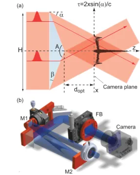
Figure 1(a) illustrates the basic principle of the autocorrela-tor. The creation of the two replica is performed by means of a Fresnel biprism.22 For the following discussion, we will consider that the Fresnel biprism has an apex angle A, a refractive index n, a thickness e0, and a height H (it will be supposed hereafter that
the laser beam is larger than the biprism, i.e., the biprism is the pupil of the optical system). The propagation of the laser pulse in the biprism leads to the creation of two identical beams cross-ing with an angle 2α in a plane parallel to the biprism input face, where α = asin[n sin β] − β and β = π/2 − A/2. The optical path difference in the two beams imposes a temporal delay given in first approximation by ∆τ = 2x sin αc , where x is the distance rel-ative to the propagation axis z. The temporal information is then directly transposed in the spatial domain, then allowing single-shot pulse duration measurements, provided that the integration times of the camera is shorter than the repetition period of the laser to be measured. The optimal distance doptat which the two beams
per-fectly spatially overlap is given by dopt = H4(tan α1 − tan β). At this
optimal distance, the temporal window ∆τmax is given by ∆τmax
= H
csin α(1 − tan α tan β). Note that these formulas are obtained
assuming that the laser pulse propagates at phase velocity in both the biprism and air, which leads to a slight underestimation of the pulse duration. This can be corrected by applying a proportionality factor κ = 1 + ω0cos α
n cos α−1 ∂n
∂ωto the retrieved pulse duration that takes
into account the fact that the pulse envelope propagates at the group velocity.
FIG. 1. (a) Principle of the autocorrelator BOAR device. The black line is a typical experimental two-photon absorption signal recorded by using the camera. (b) Experimental setup. The two cylindrical mirrors M1 and M2 (f = −25 mm and f = 125 mm, respectively) are used for increasing the beam size in the horizontal direction by a factor of 5, and FB is the Fresnel biprism.
B. Two-photon absorption 1. General formulas
The optical autocorrelation is performed by two-photon absorption in a camera having a pixel size dx and a number of pix-els N along x placed at the distance d from the biprism output. The bandgap Ug of the semiconductor material composing the camera
pixels is chosen in the interval hcλ < Ug< 2hcλ, where h is the Planck
constant, c is the light celerity, and λ is the central wavelength to be measured. For instance, a silicon (respectively InGaAs) camera (Ug = 1.11 eV) can be used for measuring pulse duration in the
1200–2400 nm (respectively 1800–3400 nm) spectral range. Considering the total complex electric field ε(t, τ) = ε1(t)
+ ε2(t− τ) hitting a pixel of the camera, where ε1(t) = A1(t)eiω0t
[respectively ε2(t) = A2(t)eiω0t] is the field at frequency ω0= 2πc/λ
coming from the upward (respectively downward) face of the biprism, the photocurrent Iphotinduced by two-photon absorption
on one pixel of the camera is
Iphot(τ) ∝ ∫ ∣ε2(t, τ)∣2dt. (1)
Assuming a perfect balance between the two replicas’ amplitudes (A1= A2= A), the photocurrent is given by
Iphot(τ) ∝ G2(τ) + F1(τ) cos(ω0τ) + F2(τ) cos(2ω0τ), (2)
where
G2= 2 ∫ I2(t)dt + 4 ∫ I(t)I(t − τ)dt,
F1= 4 ∫ [I(t) + I(t − τ)]Re[A(t)A∗(t − τ)]dt,
F2= 2 ∫ Re(A2(t)A∗2(t − τ))dt,
(3)
and where I = |A|2is the field intensity. The contributions G2, F1, and
F2oscillate at very different frequencies (ω = 0, ω0, and 2ω0,
respec-tively). Therefore, their relative contributions to the two-photon sig-nal Iphotcan be easily distinguished by an appropriate frequency
fil-tering. One has to emphasize that the two-photon absorption signal then can be used to determine the central frequency of the laser to be measured, provided that the optical characteristics of the biprism (Apex angle and refractive index) are well determined. Note that since a part of the autocorrelation evolves with a frequency around 2ω0, the optical system has to be able to resolve the fringes at that
frequency, which imposes, in turn, an upper limit on the spatial resolution of the optical system.
2. Autocorrelation measurement assuming chirped Gaussian pulses
As every autocorrelator, an assumption about the temporal shape of the pulse has to be done so as to retrieve the pulse dura-tion from the measurement. One of the widely used assumpdura-tions is to consider a Gaussian profile, possibly with a quadratic spectral phase. More particularly, if one imposes a quadratic spectral phase Φ(ω) = K(ω − ω0)2on a Gaussian electric field with an envelope
A(t) = e −t2
σ2t [and its associated spectral amplitude ̃A(ω) ∝ e −σ2t w2
4 ], the electric field complex envelope becomes
A(t) = e −t2 σ2 tce−iat 2 , (4) with σtc = √ σ4 t+16K2 σt and a= −4 K σ4
t+16K2. According to these defini-tions, σt(respectively σtc) corresponds to the Fourier-transformed limited (respectively effective) pulse duration, and a is the temporal phase. The defined pulse durations σt(respectively σtc) are related to full width at half maximum (FWHM) Fourier-transformed limited (respectively effective) pulse durations by
∆tFWHM= √ 2 log 2 σt, (5) ∆tc,FWHM= √ 2 log 2 σtc. (6) In this case, G2, F1, and F2read, respectively,
G2(τ) = 1 + 2e −τ2 σ2 tc, F1(τ) = 4 cos aτ2 2 e −τ22(1 σ2tc+ 1 2σ2t), F2(τ) = e −τ2 σ2t. (7)
A few remarks can then be done regarding the above expressions. First, the low-frequency part of the autocorrelation (G2) gives access
to the chirped pulse duration. However, a chirped pulse and a Fourier-transform limited pulse with the same duration produce the same signal for G2. Note that G2embeds an offset induced by the
two-photon absorption signal produced by the two replicas taken individually. As discussed below, the presence of this offset can be detrimental for an accurate fit of the pulse duration. Second, the contribution oscillating around 2ω0(F2) is insensitive to the chirp
and gives access to the unchirped pulse duration. More particu-larly, the amplitude of the Fourier transform of F2corresponds to
the field spectrum amplitude in the case of Gaussian pulses. Finally, the contribution F1oscillating around ω0is sensitive to both the
pulse duration and the chirp. This function, however, is ill-suited in the case of highly chirped pulses. Indeed, this function tends to a distribution that is independent of the chirp applied to the field,
F1(τ) ∼
K→∞e
−τ2
4σ2t. (8)
As a consequence, particular care must be taken if one uses this func-tion for retrieving the effective pulse durafunc-tion, in particular if the spatial profile of the beam is noisy.
To conclude, the pulse duration can be retrieved in two dif-ferent ways. The first method is to fit G2. The drawback of this
measurement lies in the fact that this contribution is very sensi-tive to the quality of the beam profile. Indeed, since this contri-bution is a low-frequency oscillating function, it is affected by the noise coming from the beam shape imperfections. Moreover, con-trary to intensimetric single shot autocorrelators based on a type II second harmonic generation that provide a background free auto-correlation signal, G2includes not only the autocorrelation signal
but also the single SHG contribution of each replica beam. This high level of background makes the autocorrelation difficult to fit and especially when this background is noisy and not flat. Finally, the knowledge of G2does not provide any information on the frequency
chirp. The second method is to use the combination of F1 and
by fitting F2, which also gives the pulse spectrum as described
above. Then, the absolute value of the chirp parameter K, and con-sequently, the chirped pulse duration, can be determined by fit-ting F1. As mentioned above, the determination of K is limited to
moderate chirps most currently encountered in real experiments. Note that the two methods can be performed simultaneously and independently, improving then the accuracy and reliability of the measurement.
III. EXPERIMENTAL SETUP AND RESULTS
The optical design of the autocorrelator is depicted inFig. 1(b). Before the Fresnel biprism, a cylindrical reflective telescope, com-posed by two cylindrical mirrors (f =−25 mm and f = 125 mm, respectively), increases the beam size by a factor of 5 in the horizon-tal direction, direction on which the pulse duration measurement is performed. The telescope ensures that the beam size does not limit the range of pulse durations that can be measured by the autocorre-lator. Then, a A = 160○
1.7 mm thick fused silica biprism is mounted on a manual rotation stage. Using this biprism and after correction coming from the difference between phase and group velocities, the total delay range ∆τmaxis then ∆τmax≃ 5.5 ps and the optimal
dis-tance is dopt= 6.3 cm. The camera used in the autocorrelator is a
12 bit silicon CMOS camera. The minimal integration time is 35 µs, which makes the autocorrelator single-shot for lasers with a repeti-tion rate lower than 56 kHz. The camera can be externally triggered with a 14 Hz maximal frame rate. The pixel size of the camera is dx = 1.67 µm, which allows us to resolve the optical fringes in the whole spectral range of interest. In the horizontal direction, the cam-era has 3840 pixels, which gives a 6.4 mm sensor size. Accordingly, the total delay range accessible with the present camera is only 3.5 ps, while the upper limit imposed by the biprism is 5.5 ps. As a con-sequence, since the camera field of view actually limits the delay range, the biprism was placed at a distance d = 4.7 cm, i.e., before dopt. The rotation of the biprism is adjusted by aligning the
interfer-ence fringes along the vertical dimension of the camera. The signal is transferred by universal serial bus (USB) 3.0 to a computer for further processing. While the refractive index of the material com-posing the biprism (in the present case, fused silica) is well known, the calibration of the apex angle has been accurately performed prior to any autocorrelation measurements by illuminating the optical sys-tem with a HeNe laser and by measuring the interference fringes spacing on the camera. The calibration procedure finally led to A = 160.220○± 0.005○. The laser characterized during the
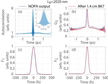
exper-iment is a commercial noncollinear optical parametric amplifier pumped by a 100 fs 800 nm chirped pulse amplified laser and delivers femtosecond laser pulses in the 1200–2400 nm wavelength region.Figure 2(a)shows a typical signal recorded with the auto-correlator for a laser wavelength set at λ0= 2020 nm. A fast Fourier
transform along the horizontal dimension allows us to easily sep-arate the three oscillating functions G2, F1, and F2that are shown
inFigs. 2(b)–2(d). At the same time, knowing that F1and F2
oscil-late around ω0 and 2ω0, respectively, the central wavelength of
the laser is estimated to be λe = 2022 nm, in very good
agree-ment with the expectations. The retrieval procedure applied to G2
gives a pulse duration (FWHM) of ∆t≃ 76 fs. Using F1and F2,
one obtains ∆t ≃ 77 fs (in very good agreement with the result obtained with G2), a Fourier-transform limited pulse duration of
FIG. 2. Autocorrelation obtained for a pulse at 2020 nm (a) and the associated oscillating function G2(b), F1(c), and F2(d). The measurement of the pulse dura-tion performed at the output of the NOPA is shown in blue line, while those done after propagation in a 1.4 cm BK7 plate is depicted in dashed red line.
∆tFTL ≃ 57 fs and a group delay dispersion (GDD) of ±1050 fs2.
Then, the same procedure has been performed after having inserted a 1.4 cm thick BK7 plate in the laser path [Figs. 2(b)–2(d)]. As expected, the contribution oscillating around 2ω0 remains
unchanged, while both G2and F1get broader than in the case
with-out the plate. The fit of G2leads to ∆t≃ 137 fs, while those of F1and
F2lead to ∆t≃ 145 fs, a Fourier-transform limited pulse duration
of ∆tFTL≃ 56.7 fs and a group delay dispersion (GDD) of ±2720 fs2.
Accordingly, one can estimate that the absolute value of the GDD introduced by the BK7 plate is about 1670 fs2. This results is in good agreement with the theoretical expectation (−1450 fs2) calcu-lated from the Sellmeier formula, in particular if one remembers that assumptions have been made on the pulse temporal and spectral profiles.
As discussed in Sec.II B 2, F2can be used for estimating the
laser spectrum. In order to confirm this, the spectrum retrieved with the autocorrelator has been compared with those actually measured with a commercial spectrometer in the case of a laser pulse centered around λ0= 1820 nm. As shown inFig. 3, the spectrum estimated by
the autocorrelator agrees well with the spectrum measured with the commercial spectrometer.
Usually, autocorrelators are sensitive to the input polarization. This is because almost all autocorrelators are based on harmonic generation, which is a strongly polarization-dependent process because of the phase-matching issue. Accordingly, in such appara-tus, the input pulse has to be linearly polarized in a particular direc-tion. Since the presented autocorrelator is based on a different pro-cess (two-photon absorption), one can wonder which polarization has to be used during the measurement. The two-photon absorption process is a priori a polarization dependent process due to the tensor nature of the two-photon absorption cross section. In order to check the polarization dependence, a Berek compensator has been inserted before the autocorrelator. This compensator allows us to impose any
FIG. 3. Laser spectrum measured with a commercial spectrometer (blue solid line) and evaluated with the BOAR (red dotted-dashed line). The black dashed line is a Gaussian fit of the spectrum measured with the spectrometer. The central wavelength of the NOPA is set to 1820 nm.
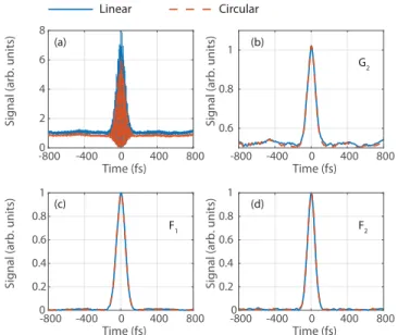
FIG. 4. Comparison between experimental autocorrelations obtained for a linearly (dashed red) and circularly (solid blue) polarized pulse (a) and the associated oscillating functions G2(b), F1(c), and F2(d) in the case of a 1400 nm laser pulse.
polarization to the pulse to be measured. A comparison between the linear and circular polarizations is depicted inFig. 4. Apart from a slightly less intense signal obtained in the circular case, the two mea-sured autocorrelations are almost identical and the fitting procedure gives the same results in both cases. Note that the autocorrelator has also been tested in the cases of elliptical polarizations and gives the same result.
IV. FULL-SPATIOTEMPORAL DYNAMICS
Since the temporal characteristics of the pulse are trans-posed in the spatial domain, the spatial beam shape can affect the
autocorrelation measurement. It is then of prime importance to characterize the spatiotemporal shape of the laser pulse in par-ticular at the plane at which the camera is placed. To this end, full spatiotemporal propagation simulations have been performed so as, first, to validate the experimental protocol and, second, in order to quantify potential limitations of the autocorrelator. In order to mimic as close as possible, the experimental configuration, a H = 2 cm fused silica biprism with 160○
apex angle, has been considered. Accordingly, the expected delay range accessible with this biprism is about ∆τmax = 5 ps and the optimal distance is
dopt≃ 6.3 cm. The central wavelength of the laser has been set to
λ0= 2 µm. The spectrum ̃E(x, ω) of the electric field E(x, t), chosen
to be as close as possible to the experimental conditions presented here, reads in good approximation after the biprism,
̃E(x,ω,d = 0) = E0e −x6 σ6pe−x2 σ2xe−σ2t(ω−ω0) 2 4 eiK(ω−ω0) 2 eiΦ(x,ω). (9) The super-Gaussian function (σp = 0.98 cm) additionally
super-imposed to the spatial profile mimics the geometrical truncation induced by the biprism, the latter being smaller than the beam size (σx = 3.4 cm) after its magnification by the cylindrical telescope.
Finally, Φ(x, ω) is the frequency-dependent phase introduced by propagation through the biprism. The latter reads
Φ(x, ω) = n(ω)ωe(x)/c + ωl(x)/c, (10) where e(x) [respectively l(x)] is the thickness of the fused silica (respectively air) crossed by the ray arriving at a given height x at the output of the biprism,
e(x) = (H 2 −
∣x∣
1− tan[α(ω)] tan β) tan β, l(x) = ∣x∣ sin β
cos[α(ω) + β].
(11)
The introduced phase then takes into account the fact that the central part of the laser pulse experiences a stronger disper-sion than the outer region because of a longer propagation path through the biprism. It also takes into account, through the fre-quency dependence of α, that the frequencies within the pulse spectrum are not deviated exactly with the same angle because of the refractive index dispersion, which leads to spatiotempo-ral couplings during the propagation after the biprism. These two parameters, together with the finite extension of the two-photon absorption band, are those limiting the measurement of very short laser pulses as it will be described below. After a propagation distance d in the air, the electric field becomes in the Fourier space,
̃E(kx, ω, d) = ̃E(kx, ω, 0)ei √
k2
air(ω)−k2xd, (12) where kair(ω) = nair(ω)ω/c, kx is the conjugate variable of x in
the reciprocal space, and nair is the frequency-dependent
refrac-tive index of the air. The spatiotemporal distribution of the electric field E(x, t, d) is then easily retrieved by an inverse Fourier-transform in both space and time.Figure 5 shows the spatiotem-poral distribution of the pulse intensity at d = dopt. The two parts
of the beam coming from the two faces of the biprism intersect and interfere at the center because they temporally overlap. Note that the part of the energy located at positive times comes from the
FIG. 5. Spatiotemporal distribution of the pulse intensity at d = dopt.
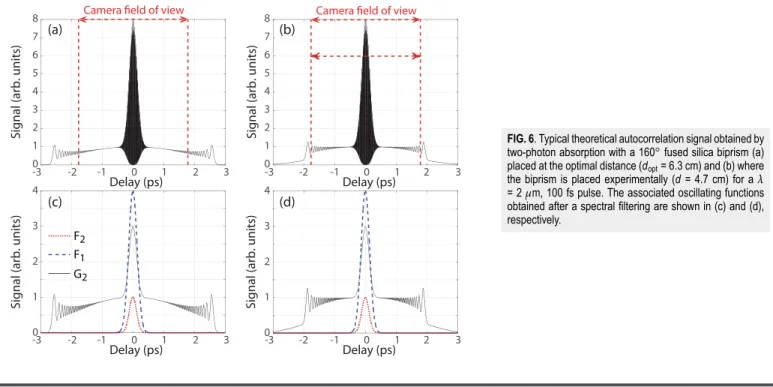
central edge of the biprism. Because of the discontinuity, it expe-riences diffraction so that oscillations can be noticed in the spa-tial profile. The photocurrent induced by two-photon absorption is then calculated by using Eq.(1)as exemplified inFig. 6(a)for d = dopt= 6.3 cm in the case of a λ0= 2 µm 100 fs Fourier
trans-form limited laser pulse. Then, the three oscillating functions F2, F1,
and G2are isolated by a spectral filtering [Fig. 6(c)] and fitted using
Eq.(7). As explained earlier, working at d = doptprovides the largest
temporal window. However, because of the Gaussian spatial profile, the offset is not uniform at this distance, which can be detrimental to correctly fit G2using Eq.(7). For solving this issue and since the
camera size actually limits the duration range that can be measured, a slightly shorter distance (d = 4.7 cm) was chosen experimentally so as to obtained a flat offset over the full temporal window. The numerical two-photon absorption signal obtained in this case and the associated oscillating functions are shown inFigs. 6(b)and6(d), respectively. Finally, the output of the propagation code has been compared to the experiments (seeFig. 7). The pulse parameters cho-sen in the simulation are those retrieved by the fit procedure during
the experiment (∆tFTL= 57 fs and ∆t = 77 fs). As shown, the
sim-ulation is in excellent agreement with the experiment, which then validates the propagation code.
A. Limitations of the autocorrelator
1. Theoretical pulse duration working range
Several distinct factors limit the pulse duration range that can be measured by means of the presented autocorrelator. The minimal Fourier-transfom-limited (FTL) pulse duration that can be mea-sured is limited by the group velocity dispersion occurring during the propagation through the biprism (even if this spectral phase can be more or less compensated by a pulse compressor). In the case of a Fourier transform limited pulse, the propagation within the biprism will make the pulse longer. More particularly, it can be shown that the quadratic phase introduced by the biprism Φpis in
good approximation, Φp=k (2)(ω 0) 2 (ω − ω0) 2 eeff, (13)
where k(2) (ω0) = ∂2k/∂ω2(ω0) is the group velocity dispersion of
the biprism material, eeff = e0(1 −2dd
opt) is the effective thickness of the biprism, and e0 = H2tan β is the thickness of the biprism
at the center. The propagation code described above was used to quantify the minimal and maximal pulse durations that can be mea-sured with our autocorrelator. For a given and known initial set of parameters (FTL pulse duration and frequency chirp), the autocor-relation signal was numerically evaluated, giving in turn the three contributions G2, F1, and F2after an appropriate spectral filtering.
Then, these extracted contributions were fitted as it is done in exper-iments. The resulting fits then give access to the evaluated FTL pulse duration and frequency chirp, which can be compared to the ini-tial set of parameters. The difference between the iniini-tial conditions
FIG. 6. Typical theoretical autocorrelation signal obtained by two-photon absorption with a 160○fused silica biprism (a) placed at the optimal distance (dopt= 6.3 cm) and (b) where the biprism is placed experimentally (d = 4.7 cm) for aλ = 2µm, 100 fs pulse. The associated oscillating functions obtained after a spectral filtering are shown in (c) and (d), respectively.
FIG. 7. (a) Comparison between the autocorrelations obtained by our propaga-tion code (red line) and the experiment (blue line). The Fourier-transform limited (respectively chirped) pulse duration of the pulse is 57 (respectively 77) fs. The central wavelength is 2020 nm. Numerical (red line) and experimental (blue line) contributions G2(b), F1(c), and F2(d) retrieved from the autocorrelations shown in (a).
and the fit of the parameters then gives the error introduced by the measurement apparatus itself.Figure 8(a)shows the relative error made by the pulse duration measurement as a function of the input pulse duration (full width at half maximum) in the conditions used during our experiment. The measurement of F2(FTL pulse
dura-tion) is almost not affected by the propagation through the biprism. This is because F2is insensitive to the chirp and consequently to the
FIG. 8. Relative error made by the fit as a function of the FTL pulse duration in the case of a fused silica (a) and NaCl (b) prism. Relative error made by the fit as a function of the initial chirp in the case of a fused silica (c) and NaCl (d) prism for a 60 fs laser pulse. The central wavelength of the pulse is 2µm.
group velocity dispersion induced in the biprism. In fact, the only thing that introduces an error is the frequency-dependence of the refraction angle at the biprism output leading to an angular chirp. However, this effect remains marginal for pulses longer than 15 fs if a fused silica biprism is used. On the contrary, the retrieved chirped pulse duration (using either G2or F1) is longer than expected, in
particular, for very short pulses and well fits the duration expected if one considers the dispersion induced by the propagation within the biprism. This means that the main effect introducing an error in the pulse measurement comes from the dispersion introduced by the propagation within the biprism and can be easily compensated during the fit algorithm. If the tolerance is set to 10%, the minimal pulse duration that can be measured in this condition (i.e., with a fused silica biprism) is about 25 fs. More particularly, setting a 10% tolerance in the pulse duration measurement and considering the biprism-induced group velocity dispersion only, one can show that the minimal pulse duration (FWHM) measurable with the present setup is given by
∆tmin(ω0) = 2 √
log(2)k(2)(ω0)eeff(1.12− 1)−1/4. (14)
Since the group-velocity dispersion of the biprism is not constant over the full spectral window, the minimal pulse duration depends on the pulse central wavelength to be measured (Fig. 9). Note that, this limit can be pushed below by the use of a NaCl biprism instead of a fused silica biprism because the former has a smaller group velocity dispersion beyond 1.6 µm.Figure 8(b)shows the error made when such a biprism is used (the apex angle of the latter has been cho-sen so as to keep the same deviation angle, i.e., A≃ 163, 3○). In
this case, the minimal theoretical pulse duration measurable is about 11 fs. As far as the maximal measurable FTL pulse duration is con-cerned, it is limited by the finite spatial expansion of the laser beam and does not depend on the biprism material as it can be noticed by comparingFigs. 8(a)and8(b)in the long pulse region. In the cho-sen configuration, the maximal pulse duration that can be measured
FIG. 9. Theoretical minimal FTL pulse duration measurable (less than 10% error in the retrieval) with the present autocorrelator as a function of the pulse central wavelength if one only considers the group velocity dispersion of the biprism (solid green line) and according to the full simulations (green squares).
is about 1 ps (FWHM) when using G2and slightly more (≃1.5 ps)
when using the combination of F1and F2. This difference is due to
the fact that the quality of the fit of G2does depend on the offset
flatness, while those of F1and F2do not. In the case of a chirped
laser pulse to be measured, the group delay dispersion induced by the propagation through the biprism impacts the retrieval of the real pulse duration, while the FTL pulse duration retrieval by means of F2remains accurate. Indeed, the quadratic phase after propagation
within the biprism Φpis
Φp= (K +
k(2)(ω0)
2 eeff)(ω − ω0)
2
, (15)
where K is the quadratic phase parameter of the pulse to be mea-sured. Depending on the relative sign of K and the group delay dispersion introduced by the biprism, the chirped pulse duration effectively measured by the autocorrelator will be either longer or shorter than the pulse duration of the input pulse.Figures 8(c)and
8(d)show the relative error of the estimation as a function of K for a 60 fs (FWHM) 2 µm laser pulse when using a fused silica or a NaCl biprism. For small K, the error is well fitted by the error introduced by the biprism dispersion. In the highly chirped case, however, the limiting factor is not the group velocity dispersion of the biprism but the finite spatial extension of the laser beam. As it is the case for FTL laser pulse, the use of G2for estimating the
laser pulse duration leads to the underestimation of the pulse dura-tion in this case. Note also that the use of a NaCl biprism leads to a smaller error on the pulse estimation also in this case. It then seems that NaCl should be preferred for the design of the autocorrelator. However, apart from the case of very short pulses (<20 fs), fused silica biprism remains a good choice, in particular if one takes into account the fact that NaCl biprisms are much more costlier than the silica one.
While the calculations presented above evaluate how the present autocorrelator modifies the pulse to be measured because of the biprism dispersion, it is common in real experiments to externally compress the pulse so as to measure the minimal pulse duration at the level of the autocorrelator itself. It is then interest-ing to evaluate the minimal pulse duration measurable if one tries to compensate the quadratic spectral phase induced by the prop-agation within the biprism. In this case, the remaining limitation will come from the higher-order dispersion terms induced by the propagation within the biprism and the angular chirp induced by the spectral dependence of the deviation angle α of the biprism (coming from the spectral dispersion of the refractive index). As shown inFig. 10(a), both the third-order dispersion and the angular chirp are more important at longer wavelengths for the fused silica biprism. As a consequence, as shown inFig. 10(b), while the the-oretical minimal pulse duration measurable by the autocorrelator after compression is slightly more than 6 fs at shorter wavelengths, it increases up to about 16 fs at 2.4 µm. However, we do not over-look the fact that for such short pulse duration, the assumption of having a Gaussian temporal and spectral profile in real experi-ment becomes relatively questionable. Comparing the results with those presented in Fig. 9, it appears that higher-order dispersion and angular chirp do not play a role below 1.3 µm. Finally, one has to emphasize that all these calculations do not take into account the finite spectral extension of the two-photon absorption band.
FIG. 10. (a) Third-order spectral dispersion of fused silica (green solid line) and frequency derivative of the deviation angle (orange dashed line). (b) Minimal pulse duration measurable with the autocorrelator if one tries to compensate for the quadratic spectral phase induced by the propagation within the biprism (orange line with red squares) and minimal pulse duration supported by the finite spectral bandwidth of the silicon (dashed blue line).
In particular, close to the upper and lower limit of the band, the minimal pulse duration measurable with our autocorrelator will be limited by the fact that a part of the pulse spectrum (which is broader and broader as the pulse duration decreases) goes beyond the spectral region of two-photon absorption.Figure 10(b)displays the minimal pulse duration supported by the two-photon absorp-tion region of the silicon. In the first approximaabsorp-tion, it has been considered that the two-photon absorption probability is flat over the region 1.15–2.45 µm and then decreases sharply out of this spec-tral range. Over the full specspec-tral region, it appears that the limiting factor of the full apparatus is indeed the finite spectral bandwidth of the two-photon absorption, even in the center of the spectral band.
2. Impact of the spatial quality of the beam
Another experimental parameter affecting the accuracy of a single-shot autocorrelator is the spatial beam quality. Indeed, since the temporal information is transposed in the spatial domain, the presence of noise in the spatial domain in turn degrades the qual-ity of the pulse duration retrieval. In order to estimate the error made when dealing with a noisy laser beam, simulations have been performed with spatial transverse profiles on which different noise amplitudes have been superimposed. The noise used in the simu-lation has not been chosen as a completely random function but behaves as 1/kx (where kx is the spatial frequency), i.e., a low
fre-quency spatial noise. This choice reproduces somehow the behavior of the noise effectively affecting amplified laser pulses as it has also been verified with our own laser system.Figure 11shows the relative error made by the fitting procedure for different noise amplitudes (keeping constant the noise spatial shape) as a function of the chirp amplitude for a 60 fs 2 µm laser pulse. The spatial profile of the
FIG. 11. Relative error made by the fit as a function of the initial chirp in the presence of a low (a), intermediate (b), and strong (c) noise in the spatial profile for a fused silica 160○biprism. The central wavelength of the pulse is 2µm, and the FTL pulse duration is 60 fs. The associated spatial electric field profile is shown in the subpanels.
electric field used in the three cases is depicted in the insets. As expected, the presence of noise is detrimental for the pulse dura-tion retrieval. At low noise amplitude [Fig. 11(a)], the error remains limited by the dispersion and finite spatial extend of the laser pulse. This is not the case anymore for intermediate and strong noise amplitudes. It can be noticed that F2is almost unaffected by the
presence of noise unlike F1and G2. There are two different
rea-sons explaining the different impact of the noise on the fit accu-racy. First, one has to remember that G2, F1, and F2evolve around
ω = 0, ω = ω0, and ω = 2ω0, respectively. This difference in the
temporal domain is transposed in the spatial domain by the use of the biprism. Since the noise mostly affects the low spatial fre-quency, it impacts more G2 than F1 and leaves F2 almost
unaf-fected. The second reason explaining why F2 is far less impacted
than the two other functions is that G2and F1extend on a longer
transverse dimension as the chirp parameter increases. As a conse-quence, they are more sensitive to the low-frequency spatial noise. Finally, as discussed above, the fit accuracy of F1decreases for long
chirped laser pulse because this function tends to a chirp unsen-sitive function as the chirp increases. This is particularly true in the presence of noise on the spatial profile. Note, however, that the impact of the noise can be decreased experimentally by a bin-ning of the pixels over the vertical dimension, which is not used for pulse duration retrieval. This averaging can be directly performed in the hardware of the camera and/or a software-performed averag-ing over the vertical dimension of the two-photon absorption signal. As shown in Fig. 11, the presence of noise in the spatial profile mostly impacts the accuracy of the fit of G2 mainly because the
fitting procedure of the latter is strongly dependent on the offset flatness.
V. EXTENSION OF THE PRINCIPLE AT LONGER WAVELENGTHS
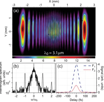
As explained above, using a silicon camera allows us to measure pulse durations for pulses located between 1200 nm and 2400 nm, which is the wavelength range of two-photon absorption of the silicon. Measuring the pulse duration of pulses located at higher wavelengths needs to adapt the materials composing the detector. A proof-of-principle experiment was performed by using an InGaAs
camera. The camera sensor is composed by 640× 512 15 µm pixels. The NaCl Fresnel biprism used in this experiment has 175○
apex angle.Figure 12(a) shows the two-photon absorption signal recorded by using the camera in the case of a 3.1 µm femtosecond laser. As shown inFig. 12(b)that displays the Fourier-transform of the signal, the three contributions G2, F1, and F2clearly appear,
which confirms the two-photon nature of the process. By fitting the oscillating functions F1 and F2 [see Fig. 12(c)], the pulse is
found to be almost Fourier-transform limited with a duration of approximately 95 fs.
FIG. 12. Pulse measurement performed atλ0= 3.1µm with a InGaAs camera. (a) Two-photon absorption signal captured with the InGaAs camera. (b) Fourier-Transform of the two-photon signal showing the three different contributions oscil-lating atω = 0, ω0, and 2ω0, respectively. (c) Temporal distribution of F1and F2. The retrieved pulse duration is about 95 fs.
VI. CONCLUSION
As a conclusion, a simple and compact single-shot autocorre-lator based on two-photon absorption in a camera and working in the 1.2–2.4 µm spectral region has been presented and analyzed in detail. The use of a Fresnel biprism for generating the two replicas makes the autocorrelator extremely robust in alignment. Moreover, it has been shown that the autocorrelator is insensitive to the input pulse polarization contrary to almost all existing autocorrelators. The interferometric nature of the autocorrelator allows us also to extract more information than with a conventional intensimetric autocorrelator. In particular, it has been shown that the pulse spec-trum, the frequency chirp, and the pulse duration can be retrieved if one assumes a particular temporal shape. Using a propagation code, the limitations of the autocorrelator have been analyzed. In partic-ular, using a fused silica biprism, it has been shown that the pulse duration range accessible with the presented configuration theoret-ically extends from 25 fs to about 1 ps. Note that the lower limit can even be lowered by using a NaCl biprism instead of a fused silica one or by using a bimirror instead of a Fresnel biprism (i.e., by using an all-reflective geometry). Nevertheless, we do not over-look that real experiments have to be performed so as to validate the theoretical expectations, in particular in the case of very short pulses. Finally, the extension to higher wavelengths (up to 3.4 µm) has been demonstrated by substituting the silicon camera by an InGaAs one.
ACKNOWLEDGMENTS
This work was supported by the Conseil Régional de Bourgogne (PARI program), the CNRS, the FEDER-FSE Bourgogne 2014/2020, the Labex ACTION program (Contract No. ANR-11-LABX-0001-01), the SATT Grand-Est, and the Carnot-ARTS. We thank the CRM-ICB (Brice Gourier, Julien Lopez, and Jean-Marc Muller) for the mechanical realization of the autocorrelator and the CRI-CCUB for CPU loan on the multiprocessor server.
REFERENCES
1
I. A. Walmsley and C. Dorrer, “Characterization of ultrashort electromagnetic pulses,”Adv. Opt. Photonics1, 308–437 (2009).
2J.-C. M. Diels, J. J. Fontaine, I. C. McMichael, and F. Simoni, “Control and
mea-surement of ultrashort pulse shapes (in amplitude and phase) with femtosecond accuracy,”Appl. Opt.24(9), 1270 (1985).
3G. Szabo, Z. Bort, and A. Muller, “Phase-sensitive single-pulse autocorrelator for
ultrashort laser pulses,”Opt. Lett.13(9), 746–748 (1988).
4
P. Langlois and E. P. Ippen, “Measurement of pulse asymmetry by three-photon-absorption autocorrelation in a GaAsP photodiode,”Opt. Lett.24, 1868–1870 (1999).
5
M. M. Karkhanehchi, C. J. Hamilton, and J. H. Marsh, “Autocorrelation mea-surements of modelocked Nd:YLF laser pulses using two-photon absorption waveguide autocorrelator,”IEEE Photonics Technol. Lett.9, 645–647 (1997).
6
C. Spielmann, L. Xu, and F. Krausz, “Measurement of interferometric autocorre-lations: Comment,”Appl. Opt.36, 2523–2525 (1997).
7
K. N. Choi and H. F. Taylor, “Novel cross-correlation technique for character-ization of subpicosecond pulses from mode-locked semiconductor lasers,”Appl. Phys. Lett.62, 1875–1877 (1993).
8
Y. Takagi, T. Kobayashi, and K. Yoshihara, “Multiple- and single-shot autocor-relator based on two-photonconductivity in semiconductors,”Opt. Lett.17(9), 658–660 (1992).
9
W. Rudolph, M. Sheik-Bahae, A. Bernstein, and L. F. Lester, “Femtosecond auto-correlation measurements based on two-photon photoconductivity in ZnSe,”Opt. Lett.22, 313–315 (1997).
10
R. Trebino, K. W. DeLong, D. N. Fittinghoff, J. N. Sweetser, M. A. Krumbugel, B. A. Richman, and D. J. Kane, “Measuring ultrashort laser pulses in the time-frequency domain using time-frequency-resolved optical gating,”Rev. Sci. Instrum.68, 3277–3295 (1997).
11
D. J. Kane and R. Trebino, “Characterization of arbitrary femtosecond pulses using frequencyresolved optical gating,”IEEE J. Quantum Electron.29, 571–579 (1993).
12
K. W. DeLong, R. Trebino, J. Hunter, and W. E. White, “Frequency-resolved optical gating with the use of second-harmonic generation,”J. Opt. Soc. Am. B11, 2206–2215 (1994).
13
K. W. DeLong and R. Trebino, “Improved ultrashort pulse-retrieval algo-rithm for frequency-resolved optical gating,”J. Opt. Soc. Am. A11, 2429–2437 (1994).
14
J. Paye, M. Ramaswamy, J. G. Fujimoto, and E. P. Ippen, “Measurement of the amplitude and phase of ultrashort light pulses from spectrally resolved autocorrelation,”Opt. Lett.18, 1946–1948 (1993).
15
D. J. Kane, A. J. Taylor, R. Trebino, and K. W. DeLong, “Single-shot measurement of the intensity and phase of a femtosecond UV laser pulse with frequency-resolved optical gating,” Opt. Lett. 19, 1061–1063 (1994).
16D. J. Kane and R. Trebino, “Single-shot measurement of the intensity and phase
of an arbitrary ultrashort pulse by using frequency-resolved optical gating,”Opt. Lett.18, 823–825 (1993).
17J. Peatross and A. Rundquist, “Temporal decorrelation of short laser pulses,” J. Opt. Soc. Am. B15, 216–222 (1998).
18
I. Amat-Roldan, I. G. Cormack, P. Loza-Alvarez, E. J. Gualda, and D. Artigas, “Ultrashort pulse characterisation with SHG collinear-FROG,”Opt. Express12, 1169–1178 (2004).
19
P. K. Bates, O. Chalus, and J. Biegert, “Ultrashort pulse characterization in the mid-infrared,”Opt. Lett.35, 1377–1379 (2010).
20R. Trebino and D. J. Kane, “Using phase retrieval to measure the intensity and
phase of ultrashort pulses: Frequency-resolved optical gating,”J. Opt. Soc. Am. A 10, 1101–1111 (1993).
21C. Iaconis and I. Walmsley, “Spectral phase interferometry for direct
electric-field reconstruction of ultrashort optical pulses,” Opt. Lett. 23, 792–794 (1998).
22P. O´shea, M. Kimmel, X. Gu, and R. Trebino, “Highly simplified device for
ultrashort-pulse measurement,”Opt. Lett.26, 932–934 (2001).
23
A. S. Radunsky, I. A. Walmsley, S.-P. Gorza, and P. Wasylczyk, “Compact spec-tral shearing interferometer for ultrashort pulse characterization,”Opt. Lett.32, 181–183 (2007).
24
V. Loriot, G. Gitzinger, and N. Forget, “Self-referenced characterization of femtosecond laser pulses by chirp scan,” Opt. Express21(21), 24879–24893 (2013).