HAL Id: halshs-00180858
https://halshs.archives-ouvertes.fr/halshs-00180858
Submitted on 22 Oct 2007HAL is a multi-disciplinary open access archive for the deposit and dissemination of sci-entific research documents, whether they are pub-lished or not. The documents may come from teaching and research institutions in France or
L’archive ouverte pluridisciplinaire HAL, est destinée au dépôt et à la diffusion de documents scientifiques de niveau recherche, publiés ou non, émanant des établissements d’enseignement et de recherche français ou étrangers, des laboratoires
On the use of nearest neighbors in finance
Nicolas Huck, Dominique Guegan
To cite this version:
Nicolas Huck, Dominique Guegan. On the use of nearest neighbors in finance. Revue de l’Association française de Finance, 2005, 26, pp.67-86. �halshs-00180858�
On the use of nearest neighbors in finance
Nicolas Huck et Guégan Dominique ∗
1
Introduction
Nearest Neighbors are a non linear non parametric forecasting method. It is based on a simple and attractive idea: pieces of time series, in the past, might have a resemblance to pieces in the future. This idea is the heart of this work and the word "resemblance" we will be longly discussed. In order to generate short term predictions, similar patterns of behavior are located in terms of nearest neighbors using a distance which is usually the Euclidean distance. The time evolution of these nearest neighbors is exploited to yield the desired prediction. Therefore, the procedure only uses a local information to forecast and makes no attempt to fit a model to the whole time series at once. The choice of the size (m) usually called the embedding dimension and of the number of neighbors (K) is an essential point of this method.
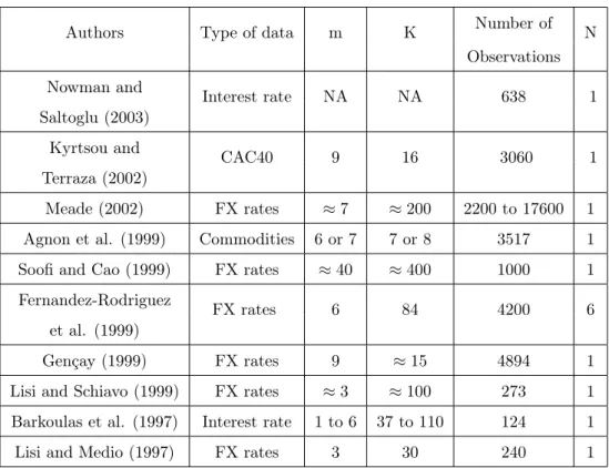
During the last years, several works used Nearest Neighbors as a forecasting method in finance. Some of the recent papers dealing with Nearest Neighbors are presented in Table ?? with their major characteristics. We indicate the type of data, the embedding dimension and the number of neighbors selected to perform predictions, the length of the series. Most of the authors works in
∗E.N.S. Cachan, Département d’Economie et Gestion et Equipe MORA-IDHE UMR CNRS 8533, 61 Avenue du President Wilson, 94235, Cachan Cedex, France, e-mail : guegan@ecogest.ens-cachan.fr
an univariate framework (N = 1). If the number of series (N ) differs from one, it means that Simultaneous Nearest Neighbors are applied. Papers are mainly concerned with foreign exchange rates. There is also some applications with stock indexes, commodities and interest rates. The sample size of the series goes from few hundreds of points to more than ten thousands observations. In few cases, we might think that the information set is maybe too small and the method hardly applicable.
Table 1
Parameters m and K are generally chosen via specific methods or via in sam-ple predictions. We observe that the selected values for m and K are most of the time too high and these high values distort the basic idea behind the Nearest Neighbors method and can lead to data snooping biases.
Here, the paper chiefly focus on the conditions of the use of the Nearest Neighbors method. We discuss the choice of the parameters m and K and the methods to select them as in Fernandez-Rodriguez et al (2003). Our ap-proach can appear new, in comparison with others works in the sense that we suggest a simple rule, based on deep empirical analysis of the method, to select parameters m and K. Our contribution can be relevant when applied to predict returns of financial assets.
If this work can be seen as relatively poor from a methodological point of view and with a lack of formalization, it is only to follow the spirit of the method and to go back to the sources which are chartist analysis and theory of graphs.
The paper is organized as follows. Section 2 presents the Nearest Neigh-bors method. Section 3, via applications, analyzes the impact of Euclidean distance and in sample predictions in the choice of the Neighbors and of the parameters m and K. The fourth Section concludes with a proposal for pa-rameters selection whom efficiency for forecasting purposes is not examined in this paper but can be considered, at least, as more meaningful than the
current approaches observed in the literature.
2
The Nearest Neighbors method
The non parametric forecasting methods such as Nearest Neighbors (Stone, 1977), Locally Weighted Regression (Cleveland, 1979) use the decomposition of the time series into histories to make predictions. In this paper, we focus on the Nearest Neighbors method but this work is also of interest for other close methods.
The intuitive idea behind this approach is based on the existence of a non linear generating process which causes patterns repeated all along a time se-ries. Thus, subsequent behaviors of the series can be used to predict behavior in the immediate future. This approach is mainly recommended to make short time predictions whether the data are non-linear. We provide an illustration of the method with two neighbors in Figure ??.
Figure 1
Let (wt)tbe a time series viewed as a sequence of histories. These are vectors
of m consecutive observations. Denote wtm the embedded histories at time t:
wmt = wt−m+1,1 . . . wt,1 .. . . .. ... wt−m+1,N . . . wt,N . (1)
In order to identify the nearest neighbors of a m history, a measure has to be defined. We use here the weighted Euclidean distance. Then, the distance between two m histories at times r and s is:
D(wrm, wms ) = N X j=1 m X i=1
αm−i+1(wr−i+1,j− ws−i+1,j)2
1/2
. (2)
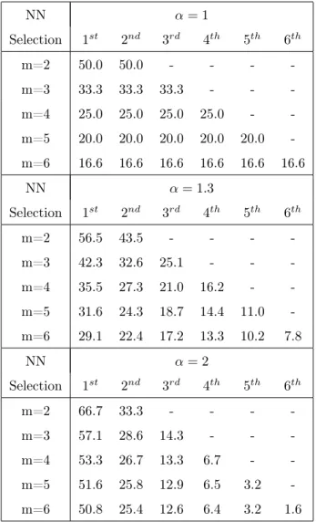
where α is a positive real number and α ≥ 1. This measure puts greater emphasis on similarity between the most recent observations as soon as α > 1.
In the literature, the value α = 1 is virtually always used. The neighbors of an history wmt are the past histories with the smallest distance.
In Table ??, we give the repartition of the weights associated to each element of an embedded history in the distance’s computation for three values of α.
Table 2
The forecasts obtained from this approach depend on the σ-algebra generated by (ws, s≤ t):
ˆ
wt+h= E[wt+h|wt, wt−1, . . . ]. (3)
The predictions are obtained by an average of the following observations in the detected nearest neighbors what some authors called "barycentric predictors". If at time t, the K nearest neighbors are identified as wm
(k,t)where k = 1, . . . , K
and w(k.,t)m refers to the last column of the kthneighbor, then the hthstep ahead forecast equals to:
ˆ wt+h,j = PK k=1γkwm(k.,t+h),j PK k=1γk ,∀j ∈ [1, . . . , N] , (4)
where γk is the weight associated to each neighbor. Predictions are thus
point predictions. In this paper, we use uniform weights to perform forecasts (γk = 1/K,∀k).
2.1 Methods to select the embedding dimension
In order to use a non parametric method like the Nearest Neighbors, the min-imal embedding dimension, m, has to be determined. It is generally chosen via in sample prediction or via phase space reconstruction methods as pre-sented now. These procedures are inherited from physics and chaos theory. Generally, there are several methods used in published literature:
• The computation of invariants (e.g., correlation dimension, Lyapunov exponents) on the attractor (e.g., Grasseberger and Procaccia, 1983),
• The singular value decomposition (Broomhead and King, 1986; Vautard and Ghil, 1989),
• The method of the false neighborhoods (Kennel et al., 1992),
• The kernel approach approach (Bosq and Guégan, 1995),
• The method of averaged false neighbors (Cao et al., 1998).
Limitations and problems in estimating the embedding dimension of a time series are numerous:
• Methods contain parameters whose interpretation is sometimes difficult or use a "subjective" judgment to choose the embedding dimension.
• The size of the time series is a key point. "While it is obvious that a short time series of low precision must lead to spurious results, we wish to argue that -even with good precision data- wrong (too low) dimension will be obtained. A similar analysis will apply to estimates of Lyapunov exponents (Eckmann and Ruelle, p 185, 1992)". A discussion on dimension calculations using small data sets can be found in Ramsey et al. (1990).
Most recent empirical works (for example: LeBaron, 1994, Kyrtsou and Ter-raza, 2002), applying various procedures to estimate the minimal embedding dimension, have shown that the returns of financial assets are highly complex. Mainly, in these articles, the estimated correlation dimension appears high and there is little (no) evidence of low-dimensional deterministic chaos. This result can be justified by the presence of noise and uncertainty which play an important role in financial markets. Evidences against low-dimensional chaos include not only high estimated (and unstable) correlation dimension but also very little evidence of out-of-sample predictability. Thus, the complexity of the financial data leads to introduce large values for the size of the neighbors in the Nearest Neighbors regression.
3
Euclidean distance and in sample predictions
This section is devoted to a deep examination of the use of Euclidean distance and in sample predictions and their consequences in the choice of the neigh-bors, their number and the embedding dimension. We try to be as pragmatic as possible and close to the spirit of the method.
3.1 Euclidean distance and neighbors selection
As a first point, we use a naive example to illustrate some properties that a neighbor must have for forecasting purposes.
Figure 2
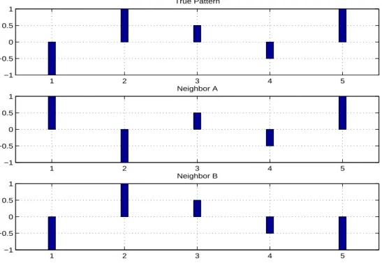
In Figure ??, we consider three pieces of a time series that we represent with bars (m = 5). The first one is the true pattern. We propose two other patterns to mimic this true pattern. The last value of the true pattern is the most recent value. We assume that the most recent values of the neighbors are the most important in a forecasting perspective. It is reasonable according to the idea of the method but implies that the series is a first order deterministic dynamical system or presents short term conditional dependence. These two points are of course highly questionable if the series is a financial time series but this is not the topic here. The values of the patterns evolve in the range [−1; 1]. As we indicate earlier in the paper, the use of Euclidean distance is the main point to select the neighbors. Considering the most common case α = 1, Neighbor B will be chosen compared to Neighbor A using Equation (??):
• Neighbor B perfectly replicates the four first values of the true pattern. The most recent value, which is the last one, is very far from the true value of its equivalent one in the true pattern.
• Neighbor A correctly matches only the last three values (the most im-portant) of the true pattern but the first two are incorrect.
Thus, we observe that the Euclidean distance between the True Pattern and the Neighbor A is higher than the one between the True Pattern and Neighbor B: Neighbor B is selected. Now if we consider a weighted Euclidean distance with α > 1 (say α = 1.3 for example), Neighbor A is selected.
This example exhibits, to our point of view, some contradictions with the idea of the Nearest Neighbors method. As soon as the forecasts are based on the immediate future of the neighbors, a neighbor, whose last value is very far from the true one (Neighbor B), can be retained whether α = 1. This does not respect the intuition underlying the nearest neighbor method. Thus, the previous selection can, in certain cases, produce very inefficient forecasts. This example points out also the importance of the choice of the parameter α in the use of the weighted Euclidean distance.
3.2 Application: RMSE and Nearest Neighbors
Among the papers we previously cited in Table ??, most of them uses in sample predictions to determine the values of the parameters, m and K, that are used for out-of-sample forecasting. The selected parameters minimize an objective function which is often the Root Mean Square Error (RMSE) or sometimes the Mean Absolute Error (MAE).
In this subsection, we perform, following the current practices observed in the literature, a selection of parameters m and K via in sample predictions. From October 1996 to October 2004, about 2000 days, we compute one step ahead daily predictions with a large range of parameters m and K with the returns of the Dow Jones Index. We use here stock market data to illustrate our method while most of the previous empirical papers we have quoted in Table ?? deals with exchange rate data. In this general discussion, the choice of the series is not important.
Raw data are used and only the stationarity in mean of the series is required. Two sizes of information sets are used: in a first step, the information set
contains the 500 last available data1
(about 2 years of daily data). In a sec-ond step, the same procedure is applied but the number of past observations for neighbors selection equals 5000 (about 20 years of daily data). In this application, we stay in the univariate case, N = 1, and use a weighted Euclid-ean distance with α = 1.3. This value reinforces the importance of the most recent elements and preserves a real weight to the first elements as Table ?? shows.
The RMSE2
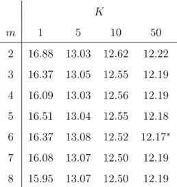
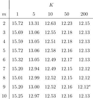
obtained with small and large data sets are provided in Tables ?? and ??. The main indication is that the RMSE seems to be decreasing func-tion of the number of neighbors. A similar relafunc-tionship between the number of neighbors and the RMSE is, for example, already mentioned in Casdagli (1992), LeBaron (1992) and Jaditz and Sayers (1998).
Table 3
Table 4
In each of our two cases, the maximum value of neighbors we test give the best results in terms of RMSE. For small data sets, the strategy with the smallest RMSE3
is obtained with m = 6 and K = 50; with large data sets, the couple of parameters, m = 9 and K = 200, appears the most efficient.
The relationship between K and the RM SE we have observed with real data can be formalized with a simple but informative theoretical example only dealing with K. Assume that (xt)t is a time series and follows a centered
Gaussian law with variance one.
Suppose we forecast the series (xt)t with a nearest neighbors regression. The
forecasting error, the RMSE, can be written, according to the number of
1
We call "T" the number of observations available for neighbors selection. The informa-tion set moves in order to keep the same size.
2
All numbers are multiplied by 1000. 3
neighbors, as: RM SEk= v u u t1 F s+F −1 X t=s (xt− ˆxt,k)2 (5)
where F is a large number of forecasts, s the date of the beginning of the fore-casting period and ˆxt,k the one step ahead prediction of xtusing k neighbors.
ˆ
xt,k, the prediction, is the mean of the future values of the neighbors. Thus,
the distribution of the forecasts and of the prediction error are given by:
ˆ xt,k ∼ N µ 0,√1 k ¶ (6) and (xt− ˆxt,k)∼ N Ã 0, r 1 +1 k ! (7)
For two different values of k, say k1 and k2, we can now conclude that:
RM SEk1 > RM SEk2, ∀k1 < k2 (8)
From a general point of view, this subsection has shown that the estimation of K via in sample predictions leads to choose high values, near or on the border of one has tabulated because the RMSE is a decreasing function of the number of neighbors. This is also true with the MAE. Concerning m, small values are rarely selected (Meade, 2002).
3.3 Application: Forecasts properties
Now choosing a couple of parameters via in sample predictions, we want to know if they are really relevant according to the spirit of the method. We analyze here the series of forecasts.
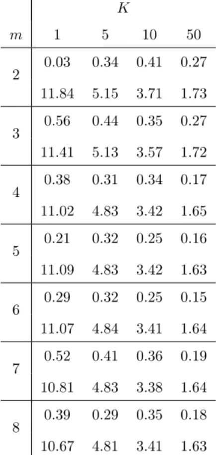
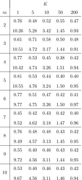
We again consider the one step ahead forecasts of the Dow Jones Index on the period October 1996 to October 2004 (about 2000 predictions). In Tables ?? and ??, we provide the mean4
(first line of each cell) and the standard deviation (second line of the cell) of the series of predictions when we forecast
4
using T = 500 and T = 5000. These results are obtained for different values of the couple (m, K).
Table 5
Table 6
Two remarks must be done looking at these tables:
• The higher the number of neighbors, the quicker the mean of the predic-tions converges to the mean value of the information set which is 0.33 with T = 500 and 0.46 with T = 5000.
• The higher the number of neighbors, the weaker the standard deviation of the series of forecasts.
In other words, if K is very large, what we should considered according to the previous subsection, the forecast, at each period, is very close to the mean of the sample which is of small interest. A similar information was in fact already given in Equation (??).
The ability to guess the future sign of returns is a widely used criteria to evaluate the performances of a forecasting method. In the case of predictions based on a large number of Nearest Neighbors, the rate of success must be examined very carefully mainly if the studied series has a trend over long period such as a stock index.
All the mean predictions we compute are positive because the value of the Dow Jones rose during the years that constitute the information set. For example, with 50 and 200 neighbors and T = 5000, about 60 and 66% of the forecasts were positive during the whole 8 years forecasting period. At the same time, only 51% of the returns of the Dow Jones were positive. As a consequence, in this application, if K is large and if the out-of-sample predictions period is bear, the rate of success is weak, the contrary occurs if the market is bull.
The selection of K via in sample predictions is thus dangerous and can lead to a meaningless use of the Nearest Neighbors method if the biggest value of K which is tested is very large.
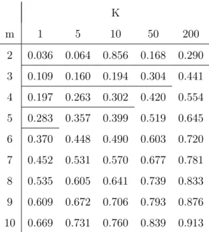
3.4 Application: Neighbors properties
The last property we focus on is the resemblance between the true patterns and the selected neighbors. The quantity (Sm,K) proposed below is based
on the Euclidean distance and on the standard deviation of the sample. It should only be seen as an empirical tool to select the neighbors as we specified in Section ?? and not to determine the optimal embedding dimension of a process. Consider the case α = 1.3 and N = 1:
Sm,K = 1 F ∗ K s+F −1 X t=s K X k=1 (m1 Pm
i=1αm−i+1(wmk,t−i+1− wt−i+1)2)1/2
σt
(9)
where F is the number of forecasts, s the date of the beginning of the fore-casting period, σtis a 500 days moving standard deviation and wmk,t−i+1refers
to the ith element of the kthneighbor with dimension m at time t. The closer
Sm,K to 0, the higher the similarity between neighbors and patterns.
Table 7
Table 8
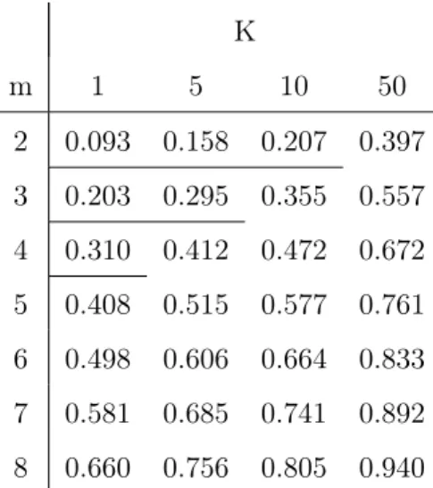
Again, we consider the Dow Jones Index and the neighbors selected to perform the predictions between October 1996 and October 2004. We define Sm,K for
K neighbors and a m embedding dimension and for two sizes of information set: T = 500 and T = 5000. The results are given in Tables ?? and ??. Naturally we observe that:
• Sm,K is an increasing function of K and m,
• If we use a large data set, this reduces Sm,K and increases the "quality"
The different experiences we made and the comparisons between neighbors and patterns indicate, empirically, that a reasonable maximum value for Sm,K
should be about 13. If this constraint is satisfied, in a very large majority of cases, the problem we describe at the beginning of this section will be avoided. Thus, we consider that the neighbors we have selected respect the "spirit" of method. This threshold value 13 builds "a sort of confidence interval" in which the resemblance between the neighbors and the patterns is important.
Considering 13 as a good threshold, we show in Tables ?? and ?? that only few couples of parameters m and K fulfill the conditions. A lower value of this threshold would, of course, increase the similarity between neighbors and the true patterns but, at the same time, it would reduce the range of acceptable parameters. Interesting parameters could be for example:
• m = 3 and K = 5 with S=500,
• m = 4 and K = 10 or m = 5 and K = 5 with S=5000.
In practice, we choose couples with intermediate values of K and m on the frontier of our region of acceptation. We think they are the most relevant because they introduce, in the regression, an information that offers a good compromise between the size, the number and the "quality" of the neighbors.
Our proposals of parameters are much lower than the values indicated in Table ?? which summarizes the m and K used in several papers. It means that, in the literature, some neighbors, selected in terms of similarity via the traditional methods, distort, "to our point of view", the idea of the nearest neighbors method. The use of small values for m is not contradictory with the non detection of low dimensional chaos because it is only due to a research of a high level of ressemblance between neighbors and patterns.
4
Concluding remarks
This paper is an interrogation on the use of the Nearest Neighbors method for time series in economics and finance. We shew that the introduction of a high embedding dimension and of an important number of neighbors, which is often observed in the literature, distorts the idea of the method. This conclusion is the result of a deep and empirical examination of the selection’s procedures of the parameters: phase space reconstruction and in sample predictions. These methods lead to an erroneous usage of the Nearest Neighbors because the neighbors are thus not near the pattern they should mimic.
We analyzed the resemblance between patterns and neighbors which is never done but should be. As a recommendation, in the univariate case, we suggest a simple empirical rule, based on the observations we made in this paper, to choose the size and the number of neighbors. We do not say that these parameters have a better predictive power than the parameters chosen with the methods generally used in the literature. The interest is that the proposed parameters are coherent according to idea of Nearest Neighbors method. If T is the length of the information set for neighbors selection, we think a reasonable value for m must be in the range [R(log(T )), R(log(T ) + 2)] where the function R rounds toward zero. About two times the values of m seems a correct value for K. From a practical point of view, these limited values of parameters m and K reduce significantly the computation time which is always interesting. The use of a weighted Euclidean distance with α > 1 is also advocate. With Simultaneous Nearest Neighbors (N > 1), a reduction of the size and/or of the number of neighbors is needed in order to preserve the quality of the neighbors because the patterns are then more complex.
A second approach that would appear less rigid and more grounded that our propositions, even if it could produce the same results to choose among the different parameters m and K, could be the development of a single and thrifty criterion as the Akaike (1974) and Schwarz (1978) criteria with parametric models. It would include the forecasting error, the size of the information set
Bibliography
Akaike, H., 1974, A new look at the statistical model identification, IEEE Transactions on Automatic Control 19, 716-723.
Agnon, Y., A. Golan., and M. Shearer, 1999, Nonparametric, Nonlinear, short-term forecasting: theory and evidence for nonlinearities in the commodity markets, Economics Letters 65, 293-299.
Barkoulas, J., C. Baum., J. Onochie, 1997, A Nonparametric Investigation of the 90-Day T-Bill Rate, Review of Financial Economics 6(2), 187-198. Bosq, D. and D. Guégan, 1995, Nonparametric Estimation of the Chaotic Function and the Invariant Measure of a Dynamical System, Statistics and Probability Letters 25, 201-212.
Broomhead, D.S., and G.P. King, 1986, Extracting qualitative dynamics from experimental data, Physica D 20, 217-236.
Cao, L., A. Mees., K. Judd, 1998, Dynamics from multivariate time series, Physica D 121, 75-88.
Cleveland, W., 1979, Robust locally weighted regression and and smoothing scatterplots, Journal of the American Statistical Association 74, 829-836. Casdagli, M., 1992, Chaos and deterministic versus stochastic nonlinear mod-eling, Journal of the Royal Statistical Society B 54, 303-328.
Eckmann, J-P., and D. Ruelle, 1992, Fundamental limitations for estimating dimensions and Lyapunov exponents in dynamical systems, Physica D 56, 185-187.
Fernandez-Rodriguez, F., S. Sosvilla-Rivero., J. Andrada-Felix, 1999, Ex-change rate forecasts with simultaneous nearest-neighbour methods: evidence from the EMS, International Journal of Forecasting 15, 383-392.
Fernandez-Rodriguez, F., S. Sosvilla-Rivero., J. Andrada-Felix, 2003, Nearest-neighbour Predictions in Foreign Exchange Markets, in Shu-Heng Chen and Paul Wang (eds), Computational Intelligence in Economics and Finance (Berlin: Physica Verlag), pp. 297-325.
Gençay, R., 1999, Linear, non-linear and essential foreign exchange rate pre-diction with simple trading rules, Journal of International Economics 47, 91-107.
Grassberger, P., and I. Procaccia, 1983, Measuring the strangeness series of strange attractors, Physica D 9, 189-208.
Jaditz, T., and C. Sayers., 1998, Out of sample forecast performance as a test for nonlinearity in time series, Journal of Business and Economic Statistics 16, 110-117.
Kennel, M., R. Brown., H. Abarbanel, 1992, Determining embedding dimen-sion for phase-space reconstruction using a geometrical construction, Physical Review A 45, 3403-3411.
Kyrtsou, C. and M. Terraza, 2002, Stochastic chaos or ARCH effects in stock series? A comparative study, International Review of Financial Analysis 11, 407-431.
LeBaron, B., 1992, Forecast improvements using a volatility index, Journal of Applied Econometrics 7, 137-149.
LeBaron, B., 1994, Chaos and Nonlinear Forecastability in Economics and Finance, Working Paper, Department of Economics, University of Wisconsin. Lisi, F. and A. Medio, 1997, Is a random walk the best exchange rate predic-tor? International Journal of Forecasting 13, 255-267.
Lisi, F. and R. Schiavo, 1999, A comparison between neural networks and chaotic models for exchange rate prediction, Computational Statistics & Data Analysis 30, 87-102.
Meade, M., 2002, A comparison of the accuracy of short term foreign exchange forecasting methods, International Journal of Forecasting 18 , 67-83.
Nowman, B. and B. Saltoglu, 2003, Continuous time and nonparametric mod-elling of U.S. interest rate models, International Review of Financial Analysis 12, 25-34.
Ramsey, J.B., P. Rothman., and C. L. Sayers, 1990, The statistical properties of dimension calculations using small data sets: Some economic applications,
International Economic Review 31, 991-1020.
Schwarz, G., 1978, Estimating the dimension of a model, Annals of Statistics 6, 461-464.
Soofi, A. and L. Cao, 1999, Nonlinear deterministic forecasting of daily Peseta-Dollar exchange rate, Economics Letters 62, 175-180.
Stone, C.J., 1977, Consistent nonparametric regression, Annals of Statistics 5, 595-645.
Vautard, R., M. Ghil, 1989, Singular spectrum analysis in nonlinear dynamics with applications to paleoclimatic time series, Physica D 35, 395-424.
Authors Type of data m K Number of N Observations
Nowman and Interest rate NA NA 638 1
Saltoglu (2003) Kyrtsou and
CAC40 9 16 3060 1
Terraza (2002)
Meade (2002) FX rates ≈ 7 ≈ 200 2200 to 17600 1 Agnon et al. (1999) Commodities 6 or 7 7 or 8 3517 1
Soofi and Cao (1999) FX rates ≈ 40 ≈ 400 1000 1
Fernandez-Rodriguez FX rates 6 84 4200 6
et al. (1999)
Gençay (1999) FX rates 9 ≈ 15 4894 1
Lisi and Schiavo (1999) FX rates ≈ 3 ≈ 100 273 1
Barkoulas et al. (1997) Interest rate 1 to 6 37 to 110 124 1
Lisi and Medio (1997) FX rates 3 30 240 1
Table 1: Some papers dealing with forecasting methods using neighbors on financial data sets between 1997 and 2003.
"NA" stands for Not Available. "≈" indicates that several series or variants are tested in the considered paper. We indicate a mean of the chosen parameters.
NN α = 1 Selection 1st 2nd 3rd 4th 5th 6th m=2 50.0 50.0 - - - -m=3 33.3 33.3 33.3 - - -m=4 25.0 25.0 25.0 25.0 - -m=5 20.0 20.0 20.0 20.0 20.0 -m=6 16.6 16.6 16.6 16.6 16.6 16.6 NN α = 1.3 Selection 1st 2nd 3rd 4th 5th 6th m=2 56.5 43.5 - - - -m=3 42.3 32.6 25.1 - - -m=4 35.5 27.3 21.0 16.2 - -m=5 31.6 24.3 18.7 14.4 11.0 -m=6 29.1 22.4 17.2 13.3 10.2 7.8 NN α = 2 Selection 1st 2nd 3rd 4th 5th 6th m=2 66.7 33.3 - - - -m=3 57.1 28.6 14.3 - - -m=4 53.3 26.7 13.3 6.7 - -m=5 51.6 25.8 12.9 6.5 3.2 -m=6 50.8 25.4 12.6 6.4 3.2 1.6
Table 2: Weighting of each element of the neighbor (%) in the computation of Euclidean distances
1 2 3 4 5 −1 −0.5 0 0.5 1 True Pattern 1 2 3 4 5 −1 −0.5 0 0.5 1 Neighbor A 1 2 3 4 5 −1 −0.5 0 0.5 1 Neighbor B
K m 1 5 10 50 2 16.88 13.03 12.62 12.22 3 16.37 13.05 12.55 12.19 4 16.09 13.03 12.56 12.19 5 16.51 13.04 12.55 12.18 6 16.37 13.08 12.52 12.17∗ 7 16.08 13.07 12.50 12.19 8 15.95 13.07 12.50 12.19
Table 3: RMSE of the forecasts with T=500 for the Dow Jones Index between October 1996 and October 2004
K m 1 5 10 50 200 2 15.72 13.31 12.63 12.23 12.15 3 15.69 13.06 12.55 12.18 12.13 4 15.59 13.05 12.51 12.18 12.13 5 15.72 13.06 12.58 12.16 12.13 6 15.32 13.05 12.49 12.17 12.13 7 15.20 12.94 12.49 12.15 12.12 8 15.01 12.99 12.52 12.15 12.12 9 15.20 13.00 12.52 12.16 12.12∗ 10 15.25 12.97 12.53 12.16 12.13
Table 4: RMSE of the forecasts with T=5000 for the Dow Jones Index between October 1996 and October 2004
K m 1 5 10 50 2 0.03 0.34 0.41 0.27 11.84 5.15 3.71 1.73 3 0.56 0.44 0.35 0.27 11.41 5.13 3.57 1.72 4 0.38 0.31 0.34 0.17 11.02 4.83 3.42 1.65 5 0.21 0.32 0.25 0.16 11.09 4.83 3.42 1.63 6 0.29 0.32 0.25 0.15 11.07 4.84 3.41 1.64 7 0.52 0.41 0.36 0.19 10.81 4.83 3.38 1.64 8 0.39 0.29 0.35 0.18 10.67 4.81 3.41 1.63
Table 5: Mean and standard deviation of the forecasts with T=500 for the Dow Jones Index between October 1996 and October 2004
K m 1 5 10 50 200 2 0.76 0.48 0.52 0.55 0.47 10.26 5.28 3.42 1.45 0.93 3 0.61 0.71 0.58 0.50 0.48 10.51 4.72 3.17 1.44 0.91 4 0.77 0.53 0.45 0.38 0.42 10.42 4.74 3.26 1.51 0.94 5 0.81 0.53 0.44 0.40 0.40 10.55 4.76 3.24 1.50 0.95 6 0.77 0.51 0.47 0.42 0.41 9.77 4.75 3.26 1.50 0.97 7 0.45 0.42 0.43 0.42 0.40 9.52 4.62 3.18 1.47 0.96 8 0.76 0.48 0.48 0.43 0.42 9.49 4.57 3.13 1.45 0.95 9 0.55 0.40 0.46 0.43 0.42 9.72 4.56 3.11 1.44 0.95 10 0.53 0.40 0.46 0.43 0.42 9.67 4.56 3.11 1.46 0.94
Table 6: Mean and standard deviation of the forecasts with T=5000 for the Dow Jones Index between October 1996 and October 2004
K m 1 5 10 50 2 0.093 0.158 0.207 0.397 3 0.203 0.295 0.355 0.557 4 0.310 0.412 0.472 0.672 5 0.408 0.515 0.577 0.761 6 0.498 0.606 0.664 0.833 7 0.581 0.685 0.741 0.892 8 0.660 0.756 0.805 0.940
Table 7: Indicator of resemblance, Sm,K, between neighbors and patterns with
K m 1 5 10 50 200 2 0.036 0.064 0.856 0.168 0.290 3 0.109 0.160 0.194 0.304 0.441 4 0.197 0.263 0.302 0.420 0.554 5 0.283 0.357 0.399 0.519 0.645 6 0.370 0.448 0.490 0.603 0.720 7 0.452 0.531 0.570 0.677 0.781 8 0.535 0.605 0.641 0.739 0.833 9 0.609 0.672 0.706 0.793 0.876 10 0.669 0.731 0.760 0.839 0.913
Table 8: Indicator of resemblance, Sm,K, between neighbors and patterns with