HAL Id: halshs-00566789
https://halshs.archives-ouvertes.fr/halshs-00566789v2
Preprint submitted on 8 Jan 2014
HAL is a multi-disciplinary open access
archive for the deposit and dissemination of sci-entific research documents, whether they are pub-lished or not. The documents may come from teaching and research institutions in France or abroad, or from public or private research centers.
L’archive ouverte pluridisciplinaire HAL, est destinée au dépôt et à la diffusion de documents scientifiques de niveau recherche, publiés ou non, émanant des établissements d’enseignement et de recherche français ou étrangers, des laboratoires publics ou privés.
Winning big but feeling no better? The effect of lottery
prizes on physical and mental health
Bénédicte H. Apouey, Andrew E. Clark
To cite this version:
Bénédicte H. Apouey, Andrew E. Clark. Winning big but feeling no better? The effect of lottery prizes on physical and mental health. 2014. �halshs-00566789v2�
WORKING PAPER N° 2009 – 09
Winning big but feeling no better? The effect of lottery prizes on
physical and mental health
Bénédicte Apouey Adrew E. Clark
JEL Codes : D1, I1, I3
Keywords: Income; Self-assessed health; Mental health; Smoking; Drinking, Conflict of interest: none declared
PARIS
-
JOURDAN SCIENCES ECONOMIQUES48, BD JOURDAN – E.N.S. – 75014 PARIS TÉL. : 33(0) 1 43 13 63 00 – FAX : 33 (0) 1 43 13 63 10
WINNING BIG BUT FEELING NO BETTER? THE EFFECT OF LOTTERY PRIZES ON PHYSICAL AND MENTAL HEALTH
B´en´edicte Apouey†
Andrew E. Clark‡
January 7, 2014
Summary
We use British panel data to determine the exogenous impact of income on a number of individual health outcomes: general health status, mental health, physical health problems, and health behaviours (drinking and smoking). Lottery winnings allow us to make causal statements regarding the effect of income on health, as the amount won by winners is largely exogenous. Positive income shocks have no significant effect on self-assessed overall health, but a significant positive effect on mental health. This result seems paradoxical on two levels. First, there is a well-known gradient in health status in cross-section data, and, second, general health should partly reflect mental health, so that we may expect both variables to move in the same direction. We propose a solution to the first apparent paradox by underlining the endogeneity of income. For the second, we show that lottery winnings are also associated with more smoking and social drinking. General health will reflect both mental health and the effect of these behaviours, and so may not improve following a positive income shock.
JEL classification: D1, I1, I3.
Keywords: Income; Self-assessed health; Mental health; Smoking; Drinking.
Conflict of interest: none declared.
†Corresponding author. Paris School of Economics - CNRS, 48 Boulevard Jourdan, 75014 Paris, France. Tel.: +33-1-43-13-63-07. Fax: +33-1-43-13-63-55. E-mail: Benedicte.Apouey@ens.fr.
1
Introduction
The relationship between individual income and health is the subject of what is by now a very substantial literature, with the broad finding that higher socio-economic status is associated with better health. This kind of relationship has now been identified in a large number of countries and for a wide variety of health variables (Deaton, 2010; Deaton and Paxson, 1999; Marmot and Bobak, 2000; Van Doorslaer et al., 1997; Winkleby et al., 1992).
While this association does indeed appear to be widespread, there is less common ground regarding its causal interpretation. That income, or socio-economic status more broadly, be correlated with health may indeed reflect a causal effect of the former on the latter. However, it is entirely possible that poor health also influence income, by reducing the ability to work for example. In addition, there are likely hidden common factors that affect both variables, such as the individual’s genetic endowment, birth weight, or the quality of the school that she attended. In this case, income and health will be correlated, but not in any causal way.
The vast majority of the existing literature is not able to distinguish between these three alternative readings of the income-health correlation. Testing the causal impact of income on health requires exogenous movements in the former, which can be identified in an instrumental or experimental setting. This is the approach to which we appeal here, using lottery winnings as an exogenous source of income variation in a large-scale panel dataset.
Most existing work on this question has used general health as the dependent variable. We are here able to provide greater detail by assessing the impact of
exogenous changes in income on a number of different health measures: self-assessed overall health, a psychological measure of mental stress (the 12-item General Health Questionnaire, or GHQ-12), physical health problems, and health-related behaviours (smoking and drinking).
The effect of income on these different health variables is far from uniform. There is first no correlation between lottery winnings and overall health. However, this lack of a relationship actually masks statistically significant correlations in different health domains. Winning big does indeed improve mental health; however, we uncover counteracting health effects with respect to risky behaviours. Those who win more on the lottery smoke more and engage in more social drinking, both of which are likely detrimental to health. The positive effect on mental health and the negative effect from risky behaviours may well sum to a negligible overall relationship between income and general health.
The remainder of the paper is organised as follows. The following section briefly summarises the related literature and discusses our approach. Section 3 presents the data we use from the British Household Panel Survey, and Section 4 discusses the identification strategies to evaluate the effect of income on health. Section 5 then contains the main results, and Section 6 presents some additional findings. Last, Section 7 concludes.
2
Background
2.1
The Causal Effect of Income on Health
Some Intuition
It is commonplace to hypothesise that higher income causes better health. If we assume that individuals maximise a utility function defined over health and other goods subject to budget and time constraints, a positive shock to income will loosen the budget constraint and will thus yield better health, if health is a normal good. However, it seems unlikely that health will also be independent of the other elements of the utility function. We can in particular imagine certain “risky behaviours” or lifestyle choices which are positively correlated with utility (and which are themselves also normal goods), but which are negatively correlated with health. In this case, higher income will have an ambiguous overall effect, by increasing smoking, drinking, calorie consumption or other risky activities which are detrimental to general health.
Findings in the Previous Literature
The positive relationship between income and health for adults is open to a num-ber of interpretations, as underlined by Smith (1999): the causality may run from income to health, from health to income, or both may be determined by hidden com-mon factors. Below, we discuss the small number of papers that have investigated this relationship by appealing to exogenous changes in income.
Elesh and Lefcowitz (1977) look at the effect of the New Jersey-Pennsylvania Negative Income Tax Experiment on various health outcomes, including the
num-ber of chronic illnesses, hospital days and work days lost, and find no effect of the experiment on health outcomes. However, the sample they use is relatively small (732 households), and they do not make any distinction between the physical, men-tal, and behavioural components of health.
Ettner (1996) also estimates the effect of income on health using American data. The health variables she uses are self-assessed health, a scale of depressive symptoms, and daily limitations due to both physical and mental difficulties. The effect of income on physical and mental health is therefore not systematically separately evaluated. She addresses the problem of reverse causality via instrumentation, using the State unemployment rate, work experience, parental education, and spousal characteristics as instruments. A substantial impact of income on all of the health variables is found, although more recent research has questioned the validity of the instruments used (Kawachi et al., 2010).
Frijters et al. (2005) analyse the relationship between income and two health variables (health satisfaction and self-assessed health). They address both reverse causality and hidden common factors, by appealing to German reunification (which resulted in a rapid and exogenous rise in average real household incomes for East Germans, but not for West Germans). The model is estimated using an original method (an ordinal fixed-effects logit regression). They find that income has a positive but only very small effect on health satisfaction and self-assessed health.
More recent work by Gardner and Oswald (2007) explores the causality running from exogenous variations in income (from medium-sized lottery wins) to changes in mental health, as measured by the GHQ. They find that money has a positive
significant effect on mental health.
Lottery winnings are an arguably under-exploited information source for the as-sessment of the effect of exogenous variations of income on health outcomes (Connor et al., 1999). One of the first systematic uses of which we are aware is Brickman et al. (1978), although in a small-sample, and cross-sectional, context. Apart from the work on health and well-being, described in this Section, they have also appeared in empirical Labour Economics. Henley (2004) considers the determinants of labour supply, and Lindh and Ohlsson (1996) and Taylor (2001) the decision to become self-employed, where lottery gains are supposed to relax liquidity constraints. Han-kins et al. (2011) use US data on lottery winners to show that winnings postpone personal bankruptcy. Both Henley (2004) and Taylor (2001) use the same database as we do, the British Household Panel Survey (BHPS). A separate literature has traced out the reaction of consumption and savings to exogenous movements in in-come. An early example is Bodkin (1959), using an unexpected National Service Life Insurance dividend paid out to World War II veterans in 1950; more recent ex-amples include Imbens et al. (2001), who appeal to differences in winnings amongst major-prize winners of the Megabucks Lottery in Massachusetts between 1984 and 1988, and Kuhn et al. (2011), who appeal to differences in winnings in the Dutch postcode lottery.
Lindahl (2005) appeals to Swedish longitudinal data and also uses lottery prizes as an exogenous shock in income. He first constructs an overall health measure comprised of both the physical and mental aspects of health. He finds a positive and significant relationship between income and this general health measure. He
then considers some of the different aspects of health separately and finds that lottery winnings have a positive and significant effect on mental health, and a non-significant effect on cardiovascular diseases, headaches, and overweight.1 This paper is of interest in the context of our work here, as it is the first to provide robust estimates of the impact of income on a variety of health outcomes. However, the sample of lottery winners used here (626) is only relatively small. In addition, the models he estimates do not control for individual fixed effects (although there is a control for health status at baseline). Finally, Lindahl does not explore the impact of lottery winnings on health behaviours. In our article, we use a larger sample of winners, we try to address individual heterogeneity by including individual fixed effects, and we consider the impact of lottery winnings on a variety of different measures of health outcomes.
Both Meer et al. (2003) and Kim and Ruhm (2012) investigate the impact of wealth on health, using inheritances as a source of exogenous movements in the former. Meer et al. (2003) use the value of inheritances received over the last five years as an instrument for the change in wealth, and consider self-assessed health, and physical or nervous disabilities which limit the individual’s ability to work. They find that wealth does not have any significant effect on health. Kim and Ruhm (2012) estimate reduced-form equations for the effect of inheritances on mortality, health status, and health behaviours in a sample of adults aged 51 and over. They find that bequests have no large health effects. One potential limitation of the use of inheritances in this context is that they likely often result from the death of a parent or close family member, and as such may well be correlated with the individual’s
own health if there is any common genetic or lifestyle component to health. It can also be argued that some inheritances are anticipated for some time beforehand (so that individuals may change their health behaviours before receiving the bequest).2 As a result, the impact of wealth on health can be underestimated. In our approach here, lottery winnings, unlike inheritances, are unlikely to be anticipated in this sense. We are also able to consider health outcomes for adults of all ages, rather than the older only, for whom an income shock may be unlikely to produce large effects.
Finally, Van Kippersluis and Galama (2013) also provide empirical evidence on the impact of an income shock on health, after developing a theoretical model that explains why wealthier individuals would engage in healthier behaviours. They esti-mate the impact of lottery winnings (in the BHPS) and inheritances (in the Health and Retirement Study) on eating, smoking, and drinking behaviours. Compared to the previous literature, Van Kippersluis and Galama (2013) include individual fixed effects to account for individual heterogeneity. Their results are similar to ours: income shocks have a detrimental impact on lifestyles. They are also able to show that this income impact varies according to the individual’s initial income and health.
2.2
Our Approach
We appeal to monetary lottery wins to try to establish a causal link between exoge-nous movements in income and changes in a number of different health outcomes.
2Kim and Ruhm (2011) explain that half of the individuals are able to predict future inheritances
We do not construct a score bringing together the different aspects of health, as we would like to see whether these latter react differently to income shocks. As such we clearly distinguish mental from physical health. Our reason for doing so comes from the results in Ruhm (2000), which called into question the notion of one holistic concept of health, in particular in relation to the economic cycle.
Some of the results in Ruhm (2000) relate various measures of US State-level health to State-level unemployment. Perhaps the most surprising finding here is that short-run recessions are associated with lower mortality rates: the common belief that physical health is worse during recessions is wrong. There are in particular fewer deaths from cardiovascular diseases, pneumonia, and motor vehicle accidents during recessions. This aggregate relationship is confirmed in regressions relating individual health outcomes to aggregate economic conditions. Using individual data from the Behavioral Risk Factor Surveillance System, Ruhm (2000, 2005) relates individual behaviours to the local unemployment rate (but not to the individual’s labour-market status). He shows that both tobacco consumption and BMI fall during short-term recessions (so that individuals are more likely to have a healthier body weight), while regular physical activity increases. Overall, physical health is shown to be counter-cyclical. However, this does not apply to all health measures. There is one cause of death that is higher during recessions: suicide. As Ruhm (2001) notes, there is “some evidence that mental health is pro-cyclical ” (p. 2). Similar results are found in the structural estimation in Adda et al. (2009). They find that higher permanent income does not affect self-reported health, blood pressure or cardiovascular diseases, with some evidence of a negative mental health effect,
and a positive correlation with the number of cigarettes smoked per day.
We take from this literature the distinction between physical and mental health, and the potential role of risky behaviours. We will carry out our investigation at an entirely microeconomic level, by correlating various individual health measures with lottery winnings in twelve waves of large-scale panel data.
3
Data
Our data come from the BHPS, the first wave of which appeared in 1991. This general survey initially covered a random sample of around 10 000 individuals in around 5500 different households in Great Britain; increased geographical coverage has pushed these figures to around 16 000 and 9000 respectively in more recent waves. We here make use of health data from waves 6 to 18 (1996-2008), and of lottery data from waves 7 to 18 (1997-2008), as harmonised lottery information is not available in either earlier waves or more recent waves. The BHPS includes a wide range of infor-mation about individual and household demographics, mental and physical health, labour-force status, employment and values. There is both entry into and exit from the panel, leading to unbalanced data. The BHPS is a household panel: all adults in the same household are interviewed separately. Further details of this survey are available at the following address: http://www.iser.essex.ac.uk/ulsc/bhps/.
The list of the variables used in our analysis of the income-health relationship appears in Table I; we describe the key ones in a little more detail below.
3.1
Health
The BHPS contains a large number of health variables; these allow us to investigate separately the relationships of income to general, mental and physical health. We have four main measures of individual health.
General Health Status
Our first health variable is the widely-used measure of self-assessed health. This comes from the question:
“Please think back over the last 12 months about how your health has been. Compared to people of your own age, would you say that your health has on the whole been...?”, with the possible responses “Excellent, Good, Fair, Poor, and Very Poor”.
In our analysis, we use a dummy for whether the individual is in “excellent” health.
This question appears in all waves of the BHPS, except for wave 9, when a special module was introduced to calculate the SF-36 health index. This does include a general self-reported health question (actually the first question in the module), which is however both differently worded (“In general would you say your health
is...”), and uses different response categories (“Excellent, Very Good, Good, Fair, and Poor”). As such, we drop wave 9 of the BHPS from our empirical analysis.
Mental Health
To measure mental health, we use a score calculated from the General Health Questionnaire (GHQ). This latter is widely-used by psychologists, epidemiologists
and medical researchers as an indicator of mental functioning. We use the Likert GHQ score, which is the sum of the responses to twelve questions on a 0 to 3 scale. See Appendix A for the details of the questions. This count is then reversed, so that higher scores indicate higher levels of well-being, and runs from 0 (all twelve responses indicating the worst psychological health) to 36 (all responses indicating the best psychological health).3
Physical Health - Health Problems
The data also contain a number of variables indicating the presence of specific health problems. Amongst these, we retain only those which describe specific phys-ical problems.
(1) Arms, legs, hands, etc. (2) Sight (3) Hearing (4) Skin conditions/allergy (5) Chest/breathing (6) Heart/blood pressure (7) Stomach or digestion (8) Diabetes.
Physical Health - Behaviours
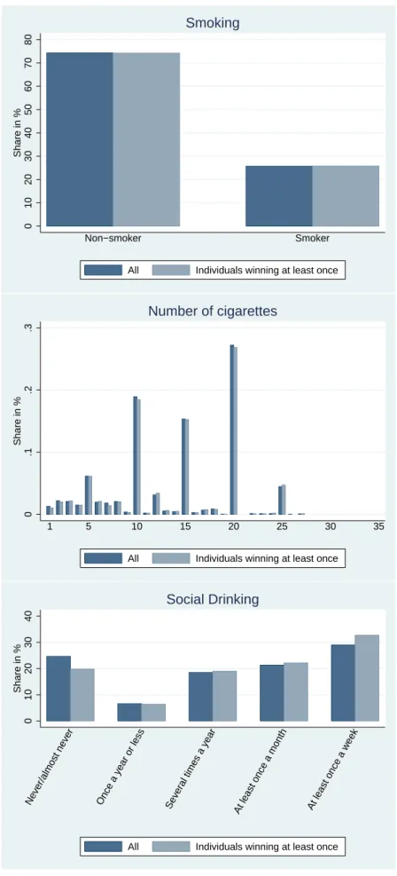
We consider two separate risky behaviours: smoking and drinking. We have two distinct smoking variables. The first is a binary variable showing whether the respondent is a current smoker, and the second picks up the number of cigarettes smoked per day.
Drinking is measured via an ordinal variable for the frequency with which the 3GHQ information from the BHPS has been used by Economists in a number of different
contexts: see Clark and Oswald (1994), Clark (2003), Ermisch et al. (2004), Gardner and Oswald (2007), and Powdthavee (2009).
respondent goes for a drink at a pub or club. This question is only asked every second year in the BHPS, with response codes as follows:
1: Never/almost never 2: Once a year or less 3: Several times a year 4: At least once a month 5: At least once a week
Figure 1 shows the distribution of these six health variables. Approximately 22% of the respondents report excellent health, and the GHQ score exhibits strong right skew. Around one-quarter of BHPS respondents are current smokers, and the modal category for social drinking is “At least once a week ”, although 25% never go out to pubs or clubs.
[Insert Figure 1 here]
3.2
Lottery Wins
We are interested in the relationship between income and these different health mea-sures. To try to identify this causal relationship, we appeal to two BHPS questions on lottery wins as a source of exogenous changes in income. These appear every year from Waves 7 to 18, and are worded as follows:
“Since September 1st (year before) have you received any payments, or payment in kind, from a win on the football pools, national lottery or other form of gambling?”
“About how much in total did you receive? (win on the football pools, national lottery or other form of gambling)”
As such, we know both whether the individual won, and how much in total they received. We have a non-negligible number of observations on lottery winners. Over the twelve BHPS waves which we use here, 10.5% of observations refer to individuals who report some winnings over the past year (11 229 “winning” observations out of 107 160 observations in total). There is no obvious time trend in the percentage of winners. Panel analysis shows that these 11 229 winning observations refer to 6 434 different individuals (out of a total of 20 474 different individuals who appear in the eleven waves of BHPS data we use). When we consider the sum of winnings over the past three years, as we do in some of our regressions, almost one-third of the sample are winners. The average win reported, expressed in real 2005 Pounds, is around £245. Six per cent of winning observations refer to sums greater than £500, and the largest win is over £200 000.
However, one potential weakness of the lottery data in the BHPS4 is that it
does not contain any direct information about the number of times (if any) that the individual has played the lottery. As such, we cannot distinguish non-players from unsuccessful players. A second point is that, both for lottery winners and playing non-winners, we do not know how much has been gambled.
On the other hand, there are significant advantages in using lottery winnings. First, as noted above, we can consider their receipt as being largely exogenous. Second, in Britain, as opposed to a number of other countries, many people play 4Which weakness also appears in the Swedish lottery data used by Lindahl (2005), but not
in the analysis of Kuhn et al. (2011), who are able to control for the number of lottery tickets purchased (although they do not consider health as an outcome).
lotteries. A recent survey-based estimate (Wardle et al., 2007) is that over two-thirds of the British participate in some kind of gambling in a given year, with 57% of the population playing the National Lottery (and almost 60% of the lat-ter playing at least once a week). The Camelot Group, who are the current Na-tional Lottery operators, report that just under £7 Billion was spent on the lottery in the 2012-2013 financial year (http://www.camelotgroup.co.uk/business/our-uk-national-lottery-operation/performance/). Consequently, there are a considerable number of lottery winners in the BHPS data.
Lottery winnings are adjusted for inflation via the consumer price index (see Appendix B) and are expressed in 2005 Pounds. In the empirical analysis, we will use the logarithm of lottery winnings, partly as income is very often entered in log form in the empirical analysis of health and well-being, and partly because the distribution of lottery winnings is, unsurprisingly, extremely right-skewed.5 The
distribution of the log of lottery winnings for winners is shown in Appendix C.
3.3
Control Variables
In line with the existing literature, our regressions include a number of fairly stan-dard control variables: age, education, labour-market and marital status, the loga-rithm of household size, the logaloga-rithm of household income, region and wave. We control for age via a series of group dummies for 20-24 years old, 25-29, ... ,75-79, and 80 years or over. The reference category is 16-19 years old. For education, we use dummies for having O-levels (reference category), A-levels, a college degree, 5Experiments using a set of lottery-winnings dummies consistently produced qualitatively
or a university degree. Labour-market status is measured using dummies for be-ing employed (reference category), unemployed, retired, or not in the labour force. The marital statuses are married (the reference category), divorced or separated, widowed, and never married. Household income comes from a derived variable, “whhnyrde”, supplied with the BHPS. This measures total household annual in-come, equivalised using the McClements before housing costs scale, and adjusted for the prices of the reference month. We use nine regions: South West (reference), London, Midlands, North West, North, Scotland, Wales, South East, and Northern Ireland.
4
Econometric Strategies
Section 3 above highlighted the exogenous income variables that are available in the BHPS. However, the way in which lottery winnings should be used in a causal regression framework merits some reflection. The underlying issue is that, while we suppose that winning the lottery is a random event, conditional on having played, the actual fact of playing the lottery may well itself be endogenous: non-players and players are likely to differ in both their observable and unobservable characteristics. As noted above, the BHPS does not include information on whether individuals play the lottery or not: we cannot distinguish players from non-players, only winners from non-winners.
One simple way of using lottery-winnings information would be to compare the health of those who have not won the lottery (which group consists of both non-players and unlucky non-players) to the health of winners. However, these two groups
are unlikely to be comparable, as the decision to play the lottery is endogenous. This poses serious problems for the interpretation of the coefficient on lottery winnings. We can of course try to condition on observable variables predicting lottery partici-pation. However, non-players and players (and therefore non-winners and winners) may also differ fundamentally in other unobservable ways. For example, non-players (who are included in the group of non-winners) may well be more risk-averse, and as a result invest more in their own health capital.
We use three different models, all of which include individual fixed effects to help correct the endogeneity issue. The fact that we appeal to fixed-effect estimation means that all estimated coefficients are identified off of within-subject variation. In our first model below, for example, the effect of any lottery win is identified by comparing the health of the same individual in periods when they had not won the lottery to their health in periods when they had.
4.1
First Model: Winners vs. Non-Winners
We first compare winning to non-winning observations (within the same individual). The specification we use is the following:
Hi,t = α + β1AnyW ini,t−k,t+ γXi,t−k−1+ νi+ ϵit, with k ≥ 0 (1)
where Hi,t represents the health outcome at date t, AnyW ini,t−k,t is a dummy for
winning any prize between t− k and t, Xi,t−k−1 denotes the control variables,
mea-sured before the win, and νi is an individual fixed effect that captures any
4.2
Second Model: Big vs. Small Wins
Second, following Gardner and Oswald (2007) and Van Kippersluis and Galama (2013), we compare larger to smaller lottery wins. The model is:
Hi,t = α + β1AnyW ini,t−k,t+ β2BigW ini,t−k,t+ γXi,t−k−1+ νi+ ϵit, with k≥ 0 (2)
where BigW ini,t−k,t is a dummy for the sum of the prizes received between t− k
and t being over £500; smaller wins are those between £1 and £500. The effect of winning under £500 then transits uniquely via β1. It turns out that the average
small win in our BHPS data is £61.64. We would not expect such small amounts of money to affect health. One interpretation of β1 is then as a placebo-type test:
consistently significant estimated values for β1 coefficient would signify a problem
with the model (via time-varying within-individual hidden common factors).
4.3
Third Model: The Amount Won
Our last specification directly includes the amount won on the lottery:
Hi,t = α + β1AnyW ini,t−k,t+ β3AnyW ini,t−k,t× Log(P rize)i,t−k,t
+γXi,t−k−1+ νi+ ϵit, with k ≥ 0
(3)
where Log(P rize)i,t−k,t denotes the demeaned log of the sum of the prizes received
corresponds to an annual win of £40: someone who wins this amount therefore has a value of AnyW ini,t,t× Log(P rize)i,t,t of zero.
4.4
Time and Consecutive Wins
In our specifications we regress health outcomes at t on the sum of prizes received between t− k and t. We estimate the models for k = 0, k = 1, and k = 2. When we use k = 0, we are interested in the immediate effect of a lottery prize on health. When we use k = 1 and k = 2, we allow the effect of lottery prizes on health to take time, while taking into account the possibility that some individuals win in consecutive years.
We imagine that any health investments may take time to bear fruit.6 A simple
model to examine the delayed impact of a prize on health k years later, would be to regress health at date t on prize at t− k. However, the estimate on the prize in this simple model might be biased, since individuals who win at t− k might also win at t− k + 1, t − k + 2,... and t. Our models, which include the sum of the prizes between t− k and t, are thus likely preferable to this simple model.
All the health equations presented above are estimated using OLS with individual fixed effects.
6Winkelmann et al. (2010) find a delayed effect of lottery winnings on a measure of well-being.
They use SOEP data to show that financial satisfaction is significantly positively correlated with the amount won by lottery winners, but only three years after the win. There is no significant effect one or two years after a win. They interpret their results as indicating deservingness: individuals only enjoy their winnings when they feel that they have deserved them. Deservingness is endogenous and can be created by the individual, but this costly investment takes time, which explains the lack of any significant effect immediately following the win. Equally, Kuhn et al. (2011) find no effect of the amount won in the Dutch postcode lottery on individual happiness six months later.
5
The Effect of Income on Health Outcomes
The following sub-sections discuss the estimation results for self-assessed health, mental health, physical health problems, and smoking and drinking in turn.
5.1
General Health Status
The regression results for the most general of our dependent variables, self-assessed health, appear in Table II. Columns (1) to (3) report the impact of lottery wins received between t− 2 and t on general health at t, columns (4) to (6) report that of lottery wins received between t−1 and t, and columns (7) to (9) that of lottery wins received at t. Columns (1), (4), and (7) contain the results of “Model 1”, whereas columns (2), (5) and (8) present those of “Model 2”, and columns (3), (6) and (9) those of “Model 3”.
The coefficients on any prize, big prizes, and on the log prize are insignificant (and almost always negative): we thus find no evidence of a positive correlation between exogenous income and general health. This is consistent with some of the previous results in the literature on the causal impact of income discussed in Section 2.1.
[Insert Table II here]
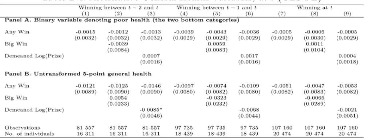
To see whether our results depend on measurement, we re-run our regressions with two alternative codings of general health: (i) a dummy variable for very poor or poor health, and (ii) the untransformed original five-point general health variable. The results appear in Appendix D, and continue to show no evidence of a positive
correlation between lottery wins and general health.7
It is likely that self-assessed health reflect both physical and mental components. Following the well-known work of Ruhm (2000), it is possible that these move in opposite directions to produce an insignificant net effect of “better economic con-ditions” (i.e. higher income) at the individual level. With this distinction in mind, we now appeal to the separate measures detailed in Section 3 above to see whether physical and mental health do indeed have sharply different relationships with ex-ogenous income. In line with Ruhm’s macro-level results, we will pay particular attention to health behaviours.
5.2
Mental Health
The results for mental health appear in Table III. There are two sets of GHQ results in this table. Those in Panel A are estimated using the full sample of observations, whereas those in Panel B refer to a restricted sample of observations for which self-assessed health and smoking are non-missing (so that the sample size in Panel B is identical to that for overall health in Table II, for example).
In Panel A, the estimated coefficients on the logarithm of the lottery prize show that positive income shocks lead to better mental health. In addition, bigger lot-tery wins between t− 2 and t also have a significant impact on well-being.8 The
coefficients in Panel B are very similar to those in Panel A, but are less precisely estimated, probably due to the smaller sample size. These results are consistent with the findings of Gardner and Oswald (2007) using the BHPS data. Our results 7Out of 30 estimated coefficients we have one which is significant: but this suggests a negative
correlation and is only significant at the ten per cent level.
in Table III show that their finding is robust to additional waves of data (we here use twelve waves as compared to the two in Gardner and Oswald), to the inclusion of individual fixed effects, to the use of several time lags, and to a more complete set of individual-level control variables (we control in addition for household size and use more detailed marital status information). The findings in Table III also represent a totally micro-econometric counterpart to the correlation between suicide and local economic activity presented in Ruhm (2000, 2001 and 2005).
The GHQ being a composite index, we can equally re-estimate the mental health equation for each of the twelve component questions listed in Section 3. The signifi-cant results are reported in Panels C to F. The positive effect of lottery winnings on well-being is particularly pronounced for the question referring to happiness (Panel F). There is also some evidence that lottery prizes affect the ability to concentrate (Panel C), sleep quality (Panel D), and the absence of pressure (Panel E).
We can confirm the effect of lottery winnings on this latter “hedonic” component of well-being by re-running our analysis using the single-item overall life satisfac-tion score available in the BHPS, which is measured on a one-to-seven scale. The regression results, presented in Panel G, show a significant correlation between the logarithm of the lottery winnings and overall life satisfaction.
“Big Wins” between t− 2 and t are positively and significantly correlated with both GHQ and life satisfaction; however, “Big Wins” received at t only do not attract significant estimated coefficients. We can interpret this in two different ways. The first is that, even with an individual fixed effect, some time-varying endogeneity remains. Individuals who are less happy than usual at time t may play more, and
thus win more at time t. This endogeneity bias is attenuated when we take all of the individual’s winnings between t− 2 and t. We cannot, of course, test for this explicitly. Second, it could take some time for big lottery winners to start enjoying their windfalls. This configuration of results has already been suggested in the literature. Kuhn et al. (2011) analyse data from the Dutch Postcode Lottery and find that winners are not happier six months after winning. Equally, Winkelmann et al. (2010) use data from the German Socio-Economic Panel to show that very large lottery wins have an impact on financial satisfaction only two years after the win. By way of contrast, they do find that gifts and inheritances have an immediate impact on satisfaction. Their explanation is that lottery winners may not immediately feel that they deserve their win, but over time they persuade themselves that they did deserve it and eventually come to enjoy their win. On the contrary, individuals straight away feel that they deserve their gifts and inheritances.
[Insert Table III here]
It may appear somewhat paradoxical that income significantly improves mental health, but at the same time has only insignificant effects on general health (as found in a number of papers, including the present). The following sub-sections propose to resolve this paradox by suggesting that income does not alleviate physical health problems, but may lead to unhealthy lifestyle outcomes.
5.3
Physical Health
To investigate the relationship between income and specific physical health prob-lems, we carry out analogous regressions to those in Table III, but replace GHQ by
information on a series of physical health problems, as listed in Section 3.
The results are given in Table IV. Given that we test for a large number of asso-ciations in this table, we account for multiple testing using a Bonferroni correction for eight comparisons (we have eight physical health problems). We thus consider that a probability value≤ 0.006 is statistically significant.
The results in Table IV reveal no significant relationships between lottery win-nings and these physical health problems once the Bonferroni correction has been applied. This might be argued to be unsurprising: higher income may well not improve individuals’ hearing, or alleviate heart and blood-pressure problems.
[Insert Table IV here]
However, one area where income might play a larger role is in the specific be-haviours that individuals undertake (i.e. the way in which they live their lives), and their ensuing health effects. In the following, we specifically consider the relationship between lottery winnings, smoking and social drinking.
5.4
Health Behaviours
The hypothesis we test in this sub-section is that positive individual income shocks may have a detrimental effect on physical health via individual lifestyles. In what follows, we specifically consider smoking and drinking.
Around 25% of our estimation sample of lottery winners report being current smokers. Panel A of Table V models the probability that the individual be a smoker. The demographic control variables here (not shown) are the same as in Table IV. The results in columns 4 through 9 show no evidence that lottery winning changes
the probability of smoking. Those in the top-left panel (columns 1 through 3) do on the contrary suggest a positive correlation between income shocks and smoking. However, our discussion in Section 4.2 suggested that a significant coefficient on the “Any Win” variable likely reflected a specification problem, as small wins should be unlikely to have a causal effect on behaviour. We believe that the results here likely reflect a hidden common factor increasing smoking probability and lottery playing at the same time.
In contrast, Panel B provides clear evidence that lottery winnings increase the probability of smoking a greater number of cigarettes.9 We repeat our analysis for social drinking in Panel C of Table V. The results indicate that the greater the lottery prize between t− 2 and t, the greater the probability of frequent social drinking.10 This effect continues to be found when we look at winnings between
t− 1 and t and at t only. In these latter results the coefficient on “Any Win” is
positive and significant as well. We believe that this effect of small winnings is less problematic here, as individuals may indeed use them to go out socially (although, as above, we would not expect a significant health effect from them).
Table V therefore shows that, rather than producing better health, higher income is broadly associated with more frequent behaviours that are commonly thought to be unhealthy. Much work has shown that, in general, higher income is associated with more favourable health outcomes. Our results here nuance this empirical fact, and are consistent with Ruhm (2000, 2001 and 2005), who considers the relationship
9Current non-smokers are dropped from this analysis.
10The estimated effect of a of a win of £20000 on the number of cigarettes is around one more
cigarette smoked per day, and that on the probability of the highest level of social drinking is around ten percentage points.
between risky health behaviours and economic booms. Ruhm’s approach is very similar to ours at one level: by relating individual (and aggregate) health outcomes to local labour market conditions, he is able to appeal to the exogeneity of the latter in determining individual health. Our results above can be read as the micro-econometric analogy of those in Ruhm. At the individual level also, exogenously higher income produces unhealthy living.
The correlations revealed by these exogenous movements are therefore largely contradictory to the commonly-noted positive link between health and social status. In reality positive (exogenous) income shocks seem to lead to lifestyle choices which are associated with worse health outcomes.11
[Insert Table V here]
6
Additional Findings
6.1
Alternative Specification
Our main specification regresses health outcomes at date t on all lottery winnings received between t− k and t, where k takes on the values 0, 1 and 2. An alternative specification is to include winnings in each year separately. We would then regress health outcomes at t on three lottery-winnings variables measured at times t− 2,
t− 1 and t. One concern here is the correlation between the same lottery variables
measured in different consecutive years, which produce larger standard errors. The 11This is arguably also reflected in having an accident. The BHPS asks all respondents whether
they had an accident over the 12 months preceding the interview. Using this variable as a health outcome, in the same way as in Table V, produces some evidence of a positive correlation with the log of the lottery prize received in the two years before the interview: big winners are more likely to end up having an accident.
estimation of models with separate winnings variables yields results that are broadly consistent with those presented here: there is no evidence of any positive significant correlation between our lottery variables and overall health, while the significant correlations between lottery winnings, on the one hand, and subjective well-being, smoking and drinking, on the other, are all positive. In these regressions (available on request), the estimated coefficients on “Big Wins” at t− 2 for GHQ are larger than those at t itself, which is consistent with the results appearing in the first panel of Table III.
6.2
Net or Gross Winnings?
The BHPS question on lottery winnings asks individuals to report “about how much
in total did you receive”. Although it is not made explicit, the most likely
interpre-tation of this question is in terms of gross winnings. Playing the lottery costs money, and it is possible that some of our winners could have actually spent more on lottery tickets over the year than they ended up winning. In general, net winnings will be smaller than gross winnings. We are interested here in the effect of an individual’s financial resources on their health and well-being. Our measure of (gross) lottery winnings then overstates the movement in the resources that they have available to them. As such, our estimated coefficient on lottery winnings is actually biased downwards. To explore this matter further, we re-estimate our third model, for prizes received between t− 2 and t, introducing not only the amount of the lottery win, but also an interaction between winnings and the fact of winning at least £1000 (we imagine that with gross winnings of at least this amount were considerably less
likely to be net losers). None of the coefficients on these interactions were close to significant, leading us to suspect that our main health results are robust.
6.3
Subgroup Analysis
To explore whether the impact of lottery winnings depends on socio-economic char-acteristics, we re-run our three specifications, for prizes received between t−2 and t, including interaction terms between lottery winnings and socioeconomic character-istics. Our results show that the effect of lottery prizes on general health and social drinking does not depend on gender. But the impact of lottery wins on the GHQ score and on the number of cigarettes smoked is greater for men than for women.
In addition, using a dummy for whether the individual is from a high-income household (i.e. his household income is above median income), we observe that the impact of winnings on general health, GHQ, the number of cigarettes smoked, and social drinking is the same for low- and high-income individuals.
Last, following Miller et al. (2009), we consider the effects of lottery winnings according to labour-market attachment. We find that the impact of lottery winnings on general health does not depend on employment status. However, there is some evidence that the effect of winnings on mental well-being and on the number of cigarettes smoked is greater for the employed.
7
Conclusion
This paper has asked whether money makes individuals healthier. While it seems well-known that the rich enjoy better health, it is far more difficult to establish the
causality of this relationship. A small recent literature has appealed to exogenous movements in income, for example lottery winnings and inheritances, to reveal either small or negligible effects of income on general health. At the same time, lottery winnings have been shown to produce better mental health.
We have suggested resolving this apparent paradox by appealing to an entirely individual-level analogy of the well-known work of Ruhm (2000, 2001 and 2005), and distinguishing between physical and mental health. Ruhm showed that recessions are associated with healthier living but more suicides. Using data on lottery winnings, “better economic conditions”, which at our micro level are picked up by greater lottery winnings, produce higher GHQ mental health scores, but also more smoking and social drinking.
The results presented here have more generally underlined three arguably central points in the analysis of health outcomes. The first is that it is unlikely that income is exogenous, so that instrumentation is essential for the understanding of causal relationships. Second, health is not a holistic concept, and we need to both be clear about what kind of health we are talking about, and be ready for the possibility that different types of health behave in very different ways. Last, the comparison of results from different levels of aggregation of both dependent and explanatory variables is a fruitful avenue of research in the economics of health and well-being.
ACKNOWLEDGEMENTS
Data from the British Household Panel Survey (BHPS) were supplied by the ESRC Data Archive. Neither the original collectors of the data nor the Archive bear any responsibility for the analysis or interpretations presented here. Financial sup-port from the US National Institute on Aging (Grant R01AG040640) is gratefully acknowledged. The paper was partially written while B´en´edicte Apouey was an Assistant Professor at the University of South Florida.
We are very grateful to the editor Jennifer Roberts and to two anonymous referees for thoughtful and constructive remarks. We thank Christophe Chamley, Thierry Debrand, Brigitte Dormont, Fabrice Etil´e, Pierre-Yves Geoffard, Hugh Gravelle, Florence Jusot, Nicolai Kristensen, Andreas Muller, Zeynep Or, Andrew Oswald, Lionel Page, Ronnie Schoeb, Hannes Schwandt, Jim Taylor and many seminar and conference participants for useful comments.
References
Adda J, Banks J, Von Gaudecker H-M, 2009. The impact of income shocks on health: evidence from cohort data. Journal of the European Economic
Asso-ciation 7: 1361-1399.
Bodkin R, 1959. Windfall income and consumption. American Economic Review
49: 602-614.
Brickman PDC, Janoff-Bulman R, 1978. Lottery winners and accident victims: is happiness relative? Journal of Personality and Social Psychology 36: 917-927. Clark AE, 2003. Unemployment as a social norm: psychological evidence from
panel data. Journal of Labour Economics 21: 323-351.
Clark AE, Oswald AJ, 1994. Unhappiness and unemployment. Economic Journal
104: 648-659.
Connor J, Rodgers A, Priest P, 1999. Randomised studies of income supplementa-tion: a lost opportunity to assess health outcomes. Journal of Epidemiology
and Community Health 53: 725-730.
Deaton A, 2010. Income, aging, health and well-being around the World: evidence from the Gallup World Poll. In Research findings in the economics of aging, David A. Wise (ed). University of Chicago Press: Chicago, pp. 235-263. Deaton AS, Paxson CH, 1999. Mortality, education, income, and inequality among
American cohorts. NBER Working Paper No. W7140.
Elesh D, Lefcowitz MJ, 1977. The effects of the New Jersey-Pennsylvania Negative Income Tax Experiment on health and health care utilization. Journal of
Health and Social Behavior 18: 391-405.
Ermisch J, Francesconi M, Pevalin DJ, 2004. Parental partnership and joblessness in childhood and their influence on young people’s outcomes. Journal of the
Royal Statistical Society Series A 167: 69-101.
Ettner S, 1996. New evidence on the relationship between income and health.
Journal of Health Economics 15: 67-86.
Frijters P, Haisken-DeNew JP, Shields MA, 2005. The causal effect of income on health: evidence from German reunification. Journal of Health Economics 24: 997-1017.
Gardner J, Oswald A, 2007. Money and mental wellbeing: a longitudinal study of medium-sized lottery wins. Journal of Health Economics 26: 49-60.
Hankins S, Paige M, Skiba M, 2011. The ticket to Easy Street? The financial consequences of winning the lottery. Review of Economics and Statistics 93: 961-969.
Henley A, 2004. House price shocks, windfall gains and hours of work: British evidence. Oxford Bulletin of Economics and Statistics 66: 439-456.
Imbens G, Rubin D, Sacerdote B, 2001. Estimating the effect of unearned in-come on labour earnings, savings, and consumption: evidence from a survey of lottery players. American Economic Review 91: 778-794.
Kawachi I, Adler NE, Dow WH, 2010. Money, schooling, and health: mechanisms and causal evidence. Annals of the New York Academy of Sciences 1186: 56-68.
Kim B, Ruhm CJ, 2012. Inheritances, health and death. Health Economics 21: 127-144.
Kuhn P, Kooreman P, Soetevent A, Kapteyn A, 2011. The effects of lottery prizes on winners and their neighbors: evidence from the Dutch Postcode Lottery.
American Economic Review 101: 2226-2247.
Lindahl M, 2005. Estimating the effect of income on health using lottery prizes as exogenous source of variation in income. Journal of Human Resources 40: 144-168.
Lindh T, Ohlsson H, 1996. Self-employment and windfall gains: evidence from the Swedish lottery. Economic Journal 106: 1515-1526.
Marmot M, Bobak M, 2000. International comparators and poverty and health in Europe. British Medical Journal 321: 1124-1128.
Meer J, Miller DL, Rosen HS, 2003. Exploring the health-wealth nexus. Journal
of Health Economics 22: 713-730.
Miller D, Page M, Stevens A, Filipski M, 2009. Why are recessions good for your health? American Economic Review 99: 122-127.
Powdthavee N, 2009. Ill-health as a household norm: evidence from other people’s health problems. Social Science and Medicine 68: 251-259.
Ruhm C, 2000. Are recessions good for your health? Quarterly Journal of
Eco-nomics 115: 617-650.
Ruhm C, 2001. Economic expansions are unhealthy. Evidence from microdata. NBER Working Paper, 8447.
Ruhm C, 2005. Healthy living in hard times. Journal of Health Economics 24: 341-363.
Taylor MP, 2001. Self-employment and windfall gains in Britain: evidence from panel data. Economica 68: 539-565.
Smith J, 1999. Healthy bodies and thick wallets: the dual relation between health and economic status. Journal of Economic Perspectives 13: 145-166.
Van Doorslaer E, Wagstaff A, Bleichrodt H, Calonge S, Gerdtham U, Gerfin M, Geurts J, Gross L, Hakkinen U, Leu RE, O’Donell O, Propper C, Puffer F, Rodriguez M, Sundberg G, Winkelhake O, 1997. Income-related inequalities in health: some international comparisons. Journal of Health Economics 16: 93-112.
Van Kippersluis H, Galama TJ, 2013. Why the rich drink more but smoke less: the impact of wealth on health behaviors. Tinbergen Institute, Working paper TI 2013-035:V.
Wardle H, Sproston K, Orford J, Erens B, Griffiths M, Constantine R, Pigott S.
British gambling prevalence survey 2007. National Centre for Social Research.
Winkelmann R, Oswald AJ, Powdthavee N, 2010. What happens to people af-ter winning the lotaf-tery? Paper presented at the 2011 EEA-ESEM Congress. Available at
http://www.eea-esem.com/files/papers/EEA-ESEM/2011/132/paper.pdf Winkleby MA, Jatulis DE, Frank E, Fortmann SP, 1992. Socioeconomic status
and health: how education, income, and occupation contribute to risk factors for cardiovascular disease. American Journal of Public Health 82: 816-820.
Table I. Definition of Analysis Variables
Health General health
Self-assessed health =1 if the individual reports excellent health Mental health
GHQ =0 for worst mental health to 36 for best mental health
GHQ-A =1 if the individual has been able to concentrate on whatever he is doing GHQ-B =1 if the individual does not lose sleep over worry
GHQ-E =1 if the individual does not feel constantly under strain GHQ-I =1 if the individual feels happy, not distressed
Life Satisfaction =1 if the individual reports low life satisfaction to 7 if the individual reports high life satisfaction Physical health
Health pb X =1 if reports health problem X Health Behaviours
Smoking =1 if the individual smokes
No. of cigarettes No. of cigarettes smoked per day, conditional on smoking Social drinking =1 if the individual goes out for a drink to a pub or club never
or almost never,
to 5 if the individual goes out for a drink to a pub or club at least once a week
Lottery
Any Win =1 if the individual has won
Big Win =1 if the individual has won over £500 Log(Prize) Logarithm of lottery prize
Control variables
Age Dummy variables for age groups:
16-19, 20-24, 25-29, 30-34, ... ,75-79, 80+ Married Reference
Divorced/Separated =1 if separated or divorced Widowed =1 if widowed
Never married =1 if never married No education Reference
O-levels =1 if has O-levels A-levels =1 if has A-levels
College degree =1 if has a College degree University degree =1 if has a University degree Employed Reference
Unemployed =1 if unemployed Retired =1 if retired
NLF =1 if not in the labour force Log(hh size) Logarithm of household size
Log(inc) Logarithm of income (real annual household income, equivalised) Region Region dummies
T able II. General Health at t (OLS-FE) Winning b et w een t− 2 and t Winning b et w een t− 1 and t Winning at t (1) (2) (3) (4) (5) (6) (7) (8) (9) An y Win -0.0032 -0.0025 -0.0040 -0.0059 -0.0055 -0.0060 -0.0023 -0.0031 -0.0020 (0.00455) (0.0046) (0.0046) (0.0041) (0.0041) (0.0041) (0.0042) (0.0043) (0.0042) Big Win -0.0099 -0.0053 0.0144 (0.0119) (0.0119) (0.0148) Demeaned Log(Prize) -0.0027 -0.0003 0.0035 (0.0023) (0.0022) (0.0026) Observ ations 81 557 81 557 81 557 97 735 97 735 97 735 107 160 107 160 107 160 No. of individuals 16 311 16 311 16 311 18 439 18 439 18 439 20 474 20 474 20 474 Notes. The mo dels include con trols for age, marital status, education, job mark et status, the logarithm of household size and income, and region and time dummies. Standard errors in paren theses. *** p < 0.01, ** p < 0.05, * p < 0.1
Table III. Mental Health at t (OLS-FE)
Winning Between t− 2 and t Winning Between t− 1 and t Winning at t
(1) (2) (3) (4) (5) (6) (7) (8) (9)
Panel A. Likert GHQ, Full Sample
Any Win 0.0582 0.0288 0.0767 0.0812* 0.0748 0.0915* 0.0686 0.0635 0.0746 (0.0538) (0.0548) (0.0544) (0.0489) (0.0499) (0.0491) (0.0499) (0.0509) (0.0500) Big Win 0.408*** 0.0935 0.0906 (0.142) (0.143) (0.178) Demeaned Log(Prize) 0.0662** 0.0586** 0.0707** (0.0281) (0.0273) (0.0312) Observations 88 078 88 078 88 078 105 754 105 754 105 754 115 668 115 668 115 668 No. of individuals 16 645 16 645 16 645 18 640 18 640 18 640 20 582 20 582 20 582
Panel B. Likert GHQ, Restricted Sample
Any Win 0.0764 0.0507 0.0896 0.0804 0.0748 0.0878* 0.0515 0.0480 0.0564 (0.0581) (0.0592) (0.0588) (0.0522) (0.0533) (0.0525) (0.0530) (0.0541) (0.0531) Big Win 0.351** 0.0790 0.0616 (0.152) (0.151) (0.187) Demeaned Log(Prize) 0.0458 0.0429 0.0596* (0.0303) (0.0290) (0.0329) Observations 81 557 81 557 81 557 97 735 97 735 97 735 107 160 107 160 107 160 No. of individuals 16 311 16 311 16 311 18 439 18 439 18 439 20 474 20 474 20 474
Panel C. GHQ-A, Ability to Concentrate
Any Win 0.0004 -0.0002 0.0004 -0.0005 -0.0014 0.0002 0.0040 0.0029 0.0047 (0.00446) (0.0045) (0.0045) (0.0040) (0.0041) (0.0040) (0.0041) (0.0042) (0.0041) Big Win 0.0092 0.0124 0.0200 (0.0117) (0.0118) (0.0148) Demeaned Log(Prize) 0.0002 0.0048** 0.0088*** (0.0023) (0.0022) (0.0025)
Panel D. GHQ-B, Sleep Quality - Not Losing Sleep Over Worry
Any Win -0.0027 -0.0050 -0.0010 0.0056 0.0055 0.0063 0.0048 0.0051 0.0049 (0.0045) (0.0046) (0.0045) (0.0041) (0.0041) (0.0041) (0.0041) (0.0042) (0.0041) Big Win 0.0310*** 0.0020 -0.0051 (0.0119) (0.0120) (0.0149) Demeaned Log(Prize) 0.0061*** 0.0039* 0.0014 (0.0023) (0.0022) (0.0026)
Panel E. GHQ-E, Absence of Pressure - Not Feeling Constantly Under Strain
Any Win -0.0039 -0.0060 -0.0019 0.0029 0.0033 0.0034 0.0034 0.0048 0.0035 (0.0050) (0.0051) (0.0050) (0.0045) (0.0046) (0.0045) (0.0046) (0.0047) (0.0046) Big Win 0.0285** -0.0054 -0.0254 (0.0132) (0.0133) (0.0166) Demeaned Log(Prize) 0.0072*** 0.0025 0.0022 (0.0026) (0.0025) (0.0029)
Panel F. GHQ-I, Feeling Happy, Not Depressed
Any Win 0.0015 -0.0005 0.0025 0.0018 0.0007 0.0027 0.0017 0.0001 0.0021 (0.0046) (0.0047) (0.0047) (0.0042) (0.0043) (0.0042) (0.0043) (0.0044) (0.0043) Big Win 0.0294** 0.0162 0.0276* (0.0123) (0.0124) (0.0154) Log(Prize) 0.0034 0.0052** 0.0047* (0.0024) (0.0023) (0.0027)
Panel G. Life Satisfaction
Any Win 0.0141 0.0065 0.0176 0.0109 0.0095 0.0130 0.0122 0.0093 0.0139 (0.0121) (0.0123) (0.0122) (0.0112) (0.0114) (0.0113) (0.0116) (0.0118) (0.0116) Big Win 0.102*** 0.0197 0.0536 (0.0316) (0.0325) (0.0416) Demeaned Log(Prize) 0.0132** 0.0115* 0.0195*** (0.0063) (0.0062) (0.0072)
Notes. The models include controls for age, marital status, education, job market status, the logarithm of household size and income, and region and time dummies. Standard errors in parentheses.
Table IV. Physical Health Problems at t (OLS-FE)
Winning between t− 2 and t Winning between t− 1 and t Winning at t
(1) (2) (3) (4) (5) (6) (7) (8) (9)
Panel A. Pb Arms, legs, hands at t
Any Win -0.0001 -0.0011 0.0014 0.0009 4.10e-05 0.0016 0.0095**# 0.0088**# 0.0098**# (0.980) (0.792) (0.738) (0.809) (0.992) (0.676) (0.0149) (0.0277) (0.0125) Big Win 0.0146 0.0127 0.0127 (0.202) (0.259) (0.360) Demeaned Log(Prize) 0.0054**# 0.0040*# 0.0032 (0.0161) (0.0641) (0.187) Panel B. Pb Sight at t Any Win 0.000169 -0.0003 0.0006 0.0024 0.0017 0.0027 0.0031 0.0025 0.0032 (0.948) (0.886) (0.807) (0.298) (0.453) (0.229) (0.174) (0.284) (0.165) Big Win 0.0075 0.0089 0.0106 (0.269) (0.180) (0.195) Demeaned Log(Prize) 0.0016 0.0022*# 0.0009 (0.226) (0.0835) (0.511) Panel C. Pb Hearing at t Any Win 0.0040 0.0042 0.0040 0.0032 0.0036 0.0030 0.0004 0.0001 0.0003 (0.118) (0.105) (0.121) (0.151) (0.117) (0.183) (0.850) (0.958) (0.892) Big Win -0.0029 -0.0052 0.0053 (0.659) (0.427) (0.509)
Demeaned Log(Prize) 4.34e-05 -0.00132 -0.0015
(0.974) (0.300) (0.292)
Panel D. Pb Skin conditions, Allergy at t
Any Win 0.0018 0.0015 0.0016 0.0033 0.0019 0.0035 0.0045 0.0039 0.0045 (0.577) (0.647) (0.612) (0.253) (0.509) (0.230) (0.124) (0.195) (0.127) Big Win 0.0041 0.0194**# 0.0110 (0.631) (0.0219) (0.293) Demeaned Log(Prize) -0.0005 0.0010 -0.0004 (0.769) (0.512) (0.804) Panel E. Pb Chest/Breathing at t
Any Win -3.73e-06 -8.16e-05 0.0007 0.0004 0.0008 0.0006 0.0019 0.0017 0.0019 (0.999) (0.978) (0.795) (0.876) (0.755) (0.819) (0.459) (0.525) (0.458)
Big Win 0.0010 -0.0060 0.0041
(0.888) (0.424) (0.657)
Demeaned Log(Prize) 0.0026*# 0.0011 8.87e-05
(0.0799) (0.444) (0.958)
Panel F. Pb Heart/Blood pressure at t
Any Win 0.0057*# 0.0059*# 0.0051 0.0033 0.0025 0.0031 0.0029 0.0023 0.0030 (0.0953) (0.0873) (0.136) (0.270) (0.415) (0.306) (0.331) (0.455) (0.326) Big Win -0.0034 0.0117 0.0110 (0.704) (0.187) (0.307) Demeaned Log(Prize) -0.0019 -0.0013 0.0004 (0.285) (0.440) (0.833) Panel G. Pb Stomach at t Any Win 0.0010 0.0007 0.0016 0.0019 0.0021 0.0020 0.0071***# 0.0061**# 0.0071***# (0.738) (0.795) (0.582) (0.468) (0.444) (0.454) (0.0092) (0.0283) (0.0093) Big Win 0.0028 -0.0021 0.0172*# (0.714) (0.786) (0.0745)
Demeaned Log(Prize) 0.0023 0.0004 -5.49e-05
(0.141) (0.781) (0.974)
Panel H. Pb Diabetes at t
Any Win -0.00031 -0.0010 0.0001 0.0003 -0.0002 0.0004 -8.20e-05 -0.0006 1.94e-05 (0.824) (0.474) (0.925) (0.765) (0.841) (0.696) (0.948) (0.619) (0.988) Big Win 0.0097***# 0.00906**# 0.0095**# (0.0080) (0.0137) (0.0306) Demeaned Log(Prize) 0.0015**# 0.0006 0.0012 (0.0353) (0.336) (0.108) Observations 81 557 81 562 81 557 97 735 97 744 97 735 107 160 107 175 107 160 No. of individuals 16 311 16 311 16 311 18 439 18 439 18 439 20 474 20 474 20 474
Notes. The models include controls for age, marital status, education, job market status, the logarithm of household size and income, and region and time dummies. Standard errors in parentheses.
*** p<0.01, ** p<0.05, * p<0.1, # When we apply the Bonferroni correction for
multiple testing (with a significance level set at P ≤ 0.006), none of the coefficients in this table is significant (at the 5% level).
T able V. Health Beha viours at t (OLS-FE) Winning b et w een t − 2 and t Winning b et w een t − 1 and t Winning at t (1) (2) (3) (4) (5) (6) (7) (8) (9) P anel A. Smoking at t, Restricted Sample An y Win 0.0084*** 0.0082*** 0.0086*** 0.0022 0.0019 0.0024 0.0003 0.0005 0.0004 (0.0025) (0.0025) (0.0025) (0.0023) (0.0023) (0.0023) (0.0024) (0.0024) (0.0024) Big Win 0.0039 0.0049 -0.0032 (0.0066) (0.0067) (0.0085) Demeaned Log(Prize) 0.0004 0.0011 0.0006 (0.0013) (0.0013) (0.0015) Observ ations 81 557 81 557 81 557 97 735 97 735 97 735 107 160 107 160 107 160 No. of individuals 16 311 16 311 16 311 18 439 18 439 18 439 20 474 20 474 20 474 P anel B. No. of Cigarettes at t, Conditional on Smoking An y Win -0.136 -0.208 -0.0849 -0.0508 -0.141 -0.0125 -0.0259 -0.0674 -0.0098 (0.136) (0.138) (0.138) (0.119) (0.122) (0.120) (0.116) (0.119) (0.116) Big Win 0.936*** 1.142*** 0.652* (0.341) (0.328) (0.386) Demeaned Log(Prize) 0.145** 0.171*** 0.132* (0.0684) (0.0636) (0.0700) Observ ations 18 847 18 847 18 847 23 247 23 247 23 247 26 603 26 603 26 603 No. of individuals 4878 4878 4878 5777 5777 5777 6626 6626 6626 P anel C. So cial Drinking at t, Y ears When Data is Av ailable An y Win 0.0206 0.0180 0.0252 0.0323** 0.0275** 0.0356*** 0.0366** 0.0314* 0.0395** (0.0158) (0.0161) (0.0159) (0.0137) (0.0140) (0.0138) (0.0158) (0.0161) (0.0158) Big Win 0.0348 0.0691* 0.0927 (0.0414) (0.0402) (0.0566) Demeaned Log(Prize) 0.0179** 0.0220*** 0.0338*** (0.0082) (0.0076) (0.0099) Observ ations 47 536 47 536 47 536 56 873 56 873 56 873 56 639 56 639 56 639 No. of individuals 16 075 16 075 16 075 17 620 17 620 17 620 19 411 19 411 19 411 Notes. The mo dels include con trols for age, marital status, education, job mark et status, the logarithm of household size and income, and region and time dummies. Standard errors in paren theses. *** p < 0.01, ** p < 0.05, * p < 0.1
Figure 1. Distribution of Health Variables 0 10 20 30 40 50 60 70 80 Share in %
Very Poor to Good Excellent
All Individuals winning at least once General Health 0 1 2 3 4 5 6 7 8 9 10 11 Share in % 0 5 10 15 20 25 30 36
All Individuals winning at least once GHQ 0 5 10 15 20 25 30 Share in %
Arms, legs, hands, etc Sight
Hearing
Skin conditions/allergy Chest/breathing
Heart/blood pressureStomach or digestion Diabetes
All Individuals winning at least once Physical Health Problems
Figure 1: Distribution of Health Variables (Continued) 0 10 20 30 40 50 60 70 80 Share in % Non−smoker Smoker
All Individuals winning at least once Smoking 0 .1 .2 .3 Share in % 1 5 10 15 20 25 30 35
All Individuals winning at least once Number of cigarettes 0 10 20 30 40 Share in %
Never/almost never Once a year or less Several times a year
At least once a month At least once a week
All Individuals winning at least once Social Drinking
Appendix A
The BHPS contains the 12-item version of the GHQ, based on the following questions. BHPS respondents are asked:
“Here are some questions regarding the way you have been feeling over the last few weeks. For each question please ring the number next to the answer that best suits the way you have felt. Have you recently....
(a) been able to concentrate on whatever you’re doing? (b) lost much sleep over worry?
(c) felt that you were playing a useful part in things? (d) felt capable of making decisions about things? (e) felt constantly under strain?
(f) felt you couldn’t overcome your difficulties?
(g) been able to enjoy your normal day-to-day activities? (h) been able to face up to problems?
(i) been feeling unhappy or depressed? (j) been losing confidence in yourself?
(k) been thinking of yourself as a worthless person? (l) been feeling reasonably happy, all things considered?” Question (a) is answered on the following four-point scale:
1: Better than usual 2: Same as usual 3: Less than usual 4: Much less than usual
Questions (b), (e), (f), (i), (j), and (k) are answered as follows: 1: Not at all
2: No more than usual 3: Rather more than usual 4: Much more than usual
And the replies to questions (c), (d), (g), (h), and (l) are on the following scale: 1: More so than usual
2: About same as usual 3: Less so than usual 4: Much less than usual.
Appendix B
Table B.I. The Consumer Price Index for the UK
Year 1997 1998 1999 2000 2001 2002 2003 2004 2005 2006 2007 2008
CPI 89.7 91.1 92.3 93.1 94.2 95.4 96.7 98.0 100.0 102.3 104.7 108.5
Appendix C
Figure C.1. Distribution of the Logarithm of Prizes for Winners
0 .1 .2 .3 .4 .5 Density 0 5 10 15 Log(Prize) kernel = epanechnikov, bandwidth = 0.1971