Montréal Septembre 2000
Série Scientifique
Scientific Series
2000s-35
Strategically Planned Behavior
in Public Good Experiments
CIRANO
Le CIRANO est un organisme sans but lucratif constitué en vertu de la Loi des compagnies du Québec. Le financement de son infrastructure et de ses activités de recherche provient des cotisations de ses organisations-membres, d’une subvention d’infrastructure du ministère de la Recherche, de la Science et de la Technologie, de même que des subventions et mandats obtenus par ses équipes de recherche.
CIRANO is a private non-profit organization incorporated under the Québec Companies Act. Its infrastructure and research activities are funded through fees paid by member organizations, an infrastructure grant from the Ministère de la Recherche, de la Science et de la Technologie, and grants and research mandates obtained by its research teams.
Les organisations-partenaires / The Partner Organizations •École des Hautes Études Commerciales
•École Polytechnique •Université Concordia •Université de Montréal
•Université du Québec à Montréal •Université Laval
•Université McGill •MEQ
•MRST
•Alcan Aluminium Ltée •AXA Canada
•Banque Nationale du Canada •Banque Royale du Canada •Bell Québec
•Bombardier •Bourse de Montréal
•Développement des ressources humaines Canada (DRHC)
•Fédération des caisses populaires Desjardins de Montréal et de l’Ouest-du-Québec •Hydro-Québec
•Imasco
•Industrie Canada
•Pratt & Whitney Canada Inc. •Raymond Chabot Grant Thornton •Ville de Montréal
© 2000 Claudia Keser. Tous droits réservés. All rights reserved.
Reproduction partielle permise avec citation du document source, incluant la notice ©.
Short sections may be quoted without explicit permission, provided that full credit, including © notice, is given to the source.
ISSN 1198-8177
Ce document est publié dans l’intention de rendre accessibles les résultats préliminaires de la recherche effectuée au CIRANO, afin de susciter des échanges et des suggestions. Les idées et les opinions émises sont sous l’unique responsabilité des auteurs, et ne représentent pas nécessairement les positions du CIRANO ou de ses partenaires.
This paper presents preliminary research carried out at CIRANO and aims at encouraging discussion and comment. The observations and viewpoints expressed are the sole responsibility of the authors. They do not necessarily represent positions of CIRANO or its partners.
Strategically Planned Behavior in Public Good Experiments
*Claudia Keser
†Résumé / Abstract
Les participants à une expérience ont soumis des stratégies pour jouer à un jeu de biens publics. Les stratégies ont interagi dans une simulation par ordinateur. Les participants ont eu l'opportunité de réviser et de re-soumettre leurs stratégies pour une deuxième et une troisième simulation. La contribution moyenne des stratégies au bien public a augmenté d'une simulation à l'autre. La majorité des stratégies soumises montrent le même patron de comportement. Dans la première période le participant signale sa volonté à coopérer par une contribution totale au bien public. Puis il s’aligne sur la contribution moyenne faite par les autres dans la période précédente. Dans la (les) période(s) finale(s), la coopération est abandonnée indépendamment du développement du jeu.
Subjects submitted strategies for playing a public good game. The strategies interacted with each other in a computer simulation. They could be revised and resubmitted for a second and a third simulation round. The strategies’ average contribution to the public good increased from one simulation to the next. The majority of the strategies submitted for the final simulation show the same pattern: In the first period, they signal their willingness to cooperate by contributing the entire endowment to the public good. Then, they reciprocate the others’ average contribution in the previous period. In the final period(s), cooperation is given up, whatever the history of the game.
Mots Clés : Biens publics, économie expérimentale, méthode stratégique
Keywords: Public goods, experimental economics, strategy method
JEL: C92, H41
* Corresponding Author: Claudia Keser, Institute of Statistics and Mathematical Economics, University of Karlsruhe, Building 20.21, 76128 Karlsruhe, Germany
Tel.: +49-721-608 3489 Fax: +49-721-608 4491 email: [email protected] I want to thank Claude Montmarquette and Reinhard Selten for their encouragement and many discussions. Thanks are also due to Arthur Schram and to all the participants in the experiment. Beyond submitting strategies, many of the participants made valuable comments and suggestions. I appreciate the hospitality of the Tinbergen Institute and the Center for Research in Experimental Economics and Political Decision-making (CREED) at the University of Amsterdam. Financial support by the Nederlands’ Organization for Scientific Research (NWO), the Tinbergen Institute, the European Commission (Human Capital and Mobility Program), the Deutsche Forschungsgemeinschaft (Sonder-forschungsbereich 504 at the University of Mannheim), and the Alexander von Humboldt-Foundation (Feodor-Lynen Fellowship) is gratefully acknowledged.
1. Introduction
For more than twenty years social psychologists, political scientists, and economists have been carrying out experiments in order to examine voluntary contributions to public goods. The experiments generally reveal that subjects contribute more to public goods than predicted by economic theory. However, they still contribute less than would be socially optimal. Furthermore, contributions tend to decline over time.
In this article, we present an experiment which distinguishes itself from the bulk of the previous experiments on public goods by two features. The first important feature is the application of the
strategy method of experimentation that was introduced by Selten (1967). Subjects were asked to
design strategies for playing twenty-five periods of a voluntary contributions game, a strategy being defined as a complete and exact behavioral plan prescribing a decision for any situation that may arise in the game. The submitted strategies, translated into computer code, interacted with each other in a computer simulation. The strategy method of experimentation allows us to observe strategically planned behavior of subjects in the specific voluntary contributions situation. It directly reveals subjects’ decision-making rules, which remain largely hidden in those experiments, where subjects interact spontaneously and directly with each other.
The second feature of our strategy experiment is the examination of a public good game in which, in game-theoretic terms, each player’s dominant strategy is to contribute part but not all of his endowment to the public good. This game has been introduced in a previous study (Keser 1996) examining subjects’ spontaneous behavior in the public good situation. We observed average contributions to the public good significantly above the dominant strategy solution. This is in keeping with the results of a vast literature on public good experimentation that considers situations where the dominant strategy solution prescribes for each player zero contribution to the public good (see Davis and Holt 1993 and Ledyard 1995 for surveys).1
One argument put forward by Andreoni (1988, 1995) to explain the observed overcontribution in public goods experiments is error making. In public goods experiments where the dominant strategy solution prescribes zero contribution to the public good and thus lies at the corner of the strategy space, errors necessarily lead to overcontribution. However, in Keser (1996) the dominant strategy solution lies in the interior of the strategy space. If we assume that subjects may make errors, they can make them in both directions from the dominant strategy solution. On average, errors made to both sides might cancel each other out. Thus, the overcontribution relative to the dominant strategy solution that we observed in Keser (1996) should not mainly be due to error making.2
Other frequently given interpretations with respect to the observed overcontribution to public goods are in terms of altruistic preferences, warm glow preferences, learning, or repeated game
1 Note that also Sefton and Steinberg (1996) examine a situation with a dominant strategy solution in the interior of the strategy space and obtain similar results.
2 Anderson, Goeree, and Holt (1998) apply their logit equilibrium model to the public good game examined in Keser (1996), showing that endogenous errors need not cancel each other out.
effects (see, for example, Palfrey and Prisbrey 1998 for a discussion). By altruistic preferences we
mean that a subject’s utility increases not only with his own payoff but also with the other players’ payoffs (Barro 1974; Becker 1974). Similarly, warm glow preferences imply that the pure act of contributing to a public good increases a subject’s utility (Andreoni 1990). The fundamental criticism that applies to both interpretations is based on the observation that contributions tend to decline over time. Why should altruistic or kind motives for contributing to a public good vanish?
The observed decline of contributions to a public good might result from subjects’ learning to play the dominant strategy. However, Andreoni (1988) provided evidence against this interpretation. He observed that, at an unexpected restart of a repeated public good game, subjects made significant contributions to the public good although their contribution level had been almost as low as zero by the end of the previous game.3
Repeated game effects could be characterized by strategic behavior in the sense of Kreps et al. (1982) in an incomplete information game: at the beginning of the game a fully rational player, being uncertain over the rationality of the other players, might overcontribute to the public good in order not to educate the other subjects who probably have not understood the incentives to free-ride (Andreoni 1988). Or, following Andreoni and Miller (1993), a fully rational player who is not sure whether or not the others are conditionally cooperative players (i.e., players who are willing to cooperate and overcontribute to the public good as long as the others also overcontribute) might overcontribute in early periods of the public good game in order to build a reputation of being a conditionally cooperative type himself. Such an interpretation can describe the observed contribution pattern. What should, however, be the precise specification of the player type who, in game-theoretic terms, is not fully rational?
If we want to understand what actually underlies the observed overcontribution, we need to know subjects' decision-making principles. A very straightforward way to gain access to individual decision-making principles is to directly ask for them in a strategy experiment.
In the strategy experiment, we organized three rounds of computer simulations with 50 and more strategies. The strategies were submitted by economists, psychologists, and mathematicians working in academics. For the second and third simulation round, each participant of the experiment had the opportunity to submit a revised strategy. In all three simulations, we observe over-contribution to the public good. The contribution level increases with each simulation round. While for the first simulation round the dominant strategy solution of the game was submitted seven times, this strategy had entirely disappeared by the third simulation. Analyzing the strategies submitted for the final simulation round, where the participants were most experienced with the game, we observe that more than half of the submitted strategies show the same pattern. In the first periods, participants signal their willingness to cooperate by contributing their entire token endowment to the public good. Thereafter, they reciprocate, in each period, the average contribution to the public good of the other players in the previous
period. The reciprocation often is generous in the sense that a participant tends to contribute a little more than the other players with whom he interacts. In the final periods, however, participants play the dominant strategy whatever the history of the game.4 Thus, an active attempt to cooperate with others, based on the principle of reciprocity, explains the observed overcontribution to the public good.5
We have to be aware of the fact that the decision principles revealed in the strategy experiment cannot be supposed to fully reflect the spontaneous decision-making rules that led to the specific behavior observed in Keser (1996). In the strategy experiment, subjects are forced to analyze the game, at least to some extent, and to construct decision rules for the entire game. When subjects interact spontaneously, they neither have the time nor consider it their task to analyze the game situation in detail. Decision rules may be made up from one decision to the next. We suggest that spontaneous behavior is likely to be more erratic than strategic behavior. Aspects of behavior such as feelings of sympathy or dislike toward the other subjects are likely to play a role in spontaneous behavior. We also have to take into consideration the fact that subjects in spontaneous game-playing experiments lack the opportunity to become experienced in playing the 25-period public good game. We consider the strategy experiment a complement to, not a substitute for, spontaneous game-playing experiments.
The major conclusion to be drawn from this experiment is that experienced subjects typically are willing to cooperate and actively attempt to achieve a high level of voluntary contributions to the public good. They orient their contributions toward those of the others in the previous period. In other words, they use reciprocity as an instrument to achieve cooperation. This suggests that in certain situations of economic life we might want to rethink whether government interventions to produce public goods are really necessary. Cooperation among potential consumers of a public good seems likely in long-run interactions where the interest in and the point of cooperation are clearly visible.
2. Experimental design
The experiment was organized as a series of computer tournaments with strategies submitted by subjects. The game for which the strategies were to be developed is the same as in Keser (1996). It is designed such that it has a Nash equilibrium in dominant strategies which lies in the interior of the strategy space. This property results from declining marginal benefits from investment in
4 This can be interpreted as end game behavior according to Stoecker (1983) and Selten and Stoecker (1986). It shows that the participants have well understood the individual profit maximizing incentives in the game.
5 In the literature we find some experiments to examine repeated social dilemma games under the assumption of incomplete information with respect to player types (McKelvey and Palfrey 1992; Andreoni and Miller 1993; Cooper, deJong, Forsythe, and Ross 1996; Gächter and Falk 1997). Andreoni and Miller (1993), for example, analyze prisoners' dilemma experiments searching for support of the sequential equilibrium reputation building prediction of a finitely repeated incomplete information game. They assume that with some probability the other player faced may be a tit-for-tat player. Our strategy experiment provides evidence that this type of playertranslated into the public good situation in the specific way presented abovenot only exists but even is typical among experienced subjects.
the private good.
2.1 The Game
The game belongs to the class of so-called Voluntary Contribution Mechanism (VCM) games. It is a 25-fold repetition of the following symmetric noncooperative constituent game.
There are four players, each of whom is endowed with 20 tokens. These 20 tokens have to be allocated between two activities, called A and B. The tokens may be used for either activity or distributed between the two activities. Only entire tokens may be allocated.
Let ai be the number of tokens allocated by player i to activity A, and bi the number of tokens
allocated by player i to activity B, with
ai, bi∈ {0,1,...,20}, ai + bi = 20, i = 1,...,4.
In both activities the tokens yield some payoff which is measured in Experimental Currency Units (ExCU). Activity A is a private activity individual to each player. Thus, the payoff that a player i receives from activity A depends on the number of tokens that player i allocates to this activity. A quadratic function determines player i’s payoff uAi(ai) resulting from the allocation of
ai tokens to activity A:
(2.1) uAi(ai) = 41ai - (ai)2.
Table I shows the payoff from each token allocated to activity A and the cumulative payoff for any number of tokens allocated to this activity. If a player allocates no tokens to activity A, he receives no payoff from this activity. Note that Table I, but not the payoff function (2.1), was presented to the subjects in the experiment.
Activity B is a public activity. The payoff to each player i from activity B depends on the total number of tokens allocated by the entire group to this activity. It is denoted as uBi(Σbj),
where Σbj is the sum of tokens allocated by all group members to activity B. Each token allocated
by a group member to activity B yields each member of the group a payoff of 15 ExCU. Thus, for each player i,
(2.2) uBi(Σbj) = 15Σbj.
The total payoff from both activities to a player i, ui(.), is the sum of payoffs from both activities:
(2.3) ui(ai,Σbj) = uAi(ai) + uBi(Σbj).
Since, for each player i, Σbj = bi + Σj≠ibj and bi = 20 - ai we can write
(2.4) ui(ai,Σj≠ibj) = 300 + 26ai - (ai)2 + 15Σj≠ibj.
The constituent game is repeated 25 times by the same group of four players. At the beginning of each of the 25 periods, each player of the group independently decides how to allocate the 20 tokens between the two activities. At the end of each period, each player is informed of the number of tokens used by the entire group for activity B and of his individual payoff from both activities in the current period. Then the next period begins. The decision situation is exactly the same in each period. Each player knows that the game ends after 25 periods. The total payoff of the 25-period game is determined as the sum of the payoffs in each period.
2.2 Theoretical Features
In the constituent game it is, for each player, a dominant strategy to allocate 13 tokens to activity A and 7 tokens to activity B. Maximizing, for each player i, Equation (2.4) with respect to ai
yields ai* = 13, regardless of what the other players in the group do. Inspection of Table I makes
this clear: each of the first 13 tokens allocated by a player to his private activity yields him more than the 15 ExCU he could earn per token allocated to the public activity. However, any token beyond the 13th allocated to his private activity A yields him less than 15 ExCU. Given this solution to the constituent game, the unique subgame perfect equilibrium of the 25-period game is found by backward induction. In each period, each player should contribute 7 tokens to the public activity. The resulting payoff for each player is 784 ExCU per period, or 19,600 ExCU for the 25-period game.
The subgame perfect equilibrium solution is not optimal for the entire group as such, since there is room for higher payoffs for all players. In each period, any token allocated to activity B yields the group as a whole more than what it would earn the individual player from his private activity. Thus, in the Pareto optimal solution, each group member in each period contributes all of his tokens to the public activity B. Each player earns a payoff of 1,200 ExCU per period, or 30,000 ExCU for the 25-period game.
2.3 Organization of the Experiment
I applied the strategy method of experimentation as an international computer tournament with a general invitation to participate. I mailed invitation and information brochures to academic economists, psychologists, and mathematicians around the world. Participants were asked to design, in flow-chart form, strategies for playing the 25-period game. A strategy is defined, in the game-theoretic sense, as a complete and exact behavioral plan prescribing a decision for any situation that may arise depending on the history of the game so far. I translated the submitted strategies into computer code for use in a computer simulation. In the simulation, the strategies were combined in all possible groups of four to play the 25-period game. The success of a strategy in a computer simulation was measured by its average payoff over all games in which it was involved. After the simulation, results were communicated to the participants. Each participant received an anonymous list of ranked simulation payoffs, and records of 20 randomly chosen plays in which her or his strategy was involved. The record of a play documented, for each period of the play in question, the strategy’s allocation decision, its payoff from each activity, and the number of tokens allocated by the entire group to activity B. All participants knew in advance that they would twice get the opportunity to revise their strategies for participation in a second and a third simulation round.
Unlike the spontaneous game-playing experiments described in Keser (1996), in this case I could not pay all of the participants in cash. However, at each simulation round, one of the participants was randomly chosen for cash payment according to her or his strategy’s success. The conversion rate was $1 for 200 ExCU in the first and the second simulation. It was $1 for 100 ExCU in the third simulation; this gave more importance to the final simulation than to the first two. Furthermore, the announcement that the lists of ranked simulation payoffs would be published was supposed to provide a good incentive for participants to aim at high payoffs.6 Before the first simulation round, participants could choose to participate anonymously in the experiment, but only 5 participants did so. The anonymity of the remaining participants was given up only after the final simulation round. Thus, with very few exceptions, a participant could not identify any of the other participants. Participants were from 13 different countries in Europe, America, and Asia. Fifty-nine participants submitted strategies for the first simulation, which was run in June 1994. For the second simulation, to take place in August 1994, we received 51 strategies. For the third simulation in October 1994, 50 strategies were submitted.
3. Simulation results
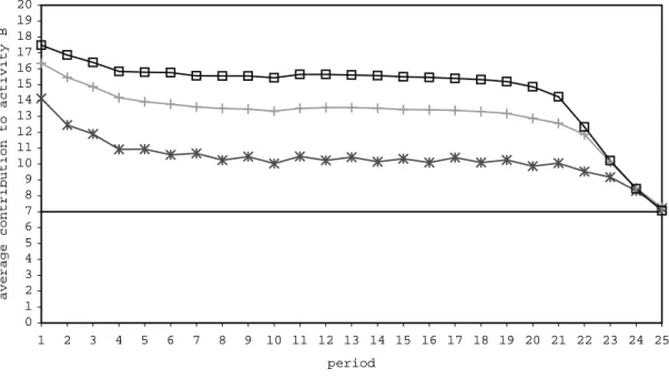
Figure 1 shows, for each simulation, the time path of the contributions made to the public activity B on average over all plays. In each simulation, contributions are, in each period, above the dominant strategy solution of 7 tokens. The contribution level continuously increases from the first to the third simulation. The average contribution to the public activity over all periods in all
6 Note that a strategy just aiming at being better than the three other strategies in the public good game is unlikely to be successful in a simulation where all strategies interact with each other in all possible group formations.
plays is 10.36 in the first simulation, 13.06 in the second simulation, and 14.67 in the third simulation. In all three simulations we observe the same pattern: initial contributions are highest. They decrease during the first few rounds, to remain then almost constant until they decrease drastically in the final rounds. The average contributions in the final round almost coincide with the dominant strategy solution.
The increasing contribution level from the first to the third simulation round is an important observation. It complements the well-known result in several oligopoly experiments that experience increases cooperation (Stoecker 1980; Benson and Faminow 1988; Keser 1993, 2000; Selten, Mitzkewitz, and Uhlich 1997).
Similar to the contribution level, the average payoff over all strategies increases with each simulation round. It is 22,118 in the first simulation, 24,518 in the second simulation, and 25,873 in the third simulation. Recall that in subgame perfect equilibrium, an individual payoff of 19,600 would be realized while in the social optimum, each player would earn 30,000 ExCU. APPENDIX A presents the list of ranked payoffs of the strategies participating in the third simulation round. It shows that the bulk of strategies fall within a fairly narrow payoff range.
4. Structure of the strategies
In the first and most important part of this section, we examine in detail the strategies which were submitted for the final simulation round. By then the subjects were somewhat experienced in playing the public good game. Furthermore, in order to give the final simulation greater weight for the subjects, the monetary incentive in that round was twice as high as in the previous simulation rounds. The decision principles of experienced subjects yield an important contribution to the understanding of human behavior in the public good situation. We are able to identify six typical properties. Each of these properties characterizes a majority of the strategies. In the second part of this section, we calculate the so-called typicity measures proposed by Selten, Mitzkewitz, and Uhlich (1997). These measures allow us to rank both properties and strategies according to how typical they are. In the third part of this section, we briefly discuss the evolution of the strategies from the first to the final decision round.
4.1 Properties of the Strategies Submitted for the Final Simulation
We identify several properties, each characterizing a majority of the strategies. It is not necessarily the case that each strategy has all of these properties. Rather, strategies tend to have these properties on average.
PROPERTY 1: Strategies are closed loop and use case distinctions.
prescribes a fixed sequence of decisions for the whole game, independently of the development of play. A closed loop strategy prescribes decisions contingent on the history of the game so far. A closed loop strategy is typically characterized by a system of simple case distinctions determining which simple decision rules to apply. Among the 50 strategies submitted for the final simulation round we identify 44 closed loop and 6 open loop strategies.
Strategies show a phase structure. Typically, different rules are specified for the first periods (initial phase), the final periods (end phase) and the intermediary periods (main phase) of the game. Closed loop strategies need to specify an initial phase. As they make decisions contingent on the past, they have to specify at least one starting value. All but two of the closed loop strategies show initial phases which last exactly as many periods as needed.
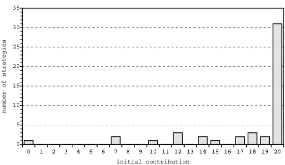
PROPERTY 2: Strategies contribute all of their endowment to the public activity in the first period.
Figure 2 depicts contributions in the first period by all strategies, whether open or closed loop. Two strategies are excluded from this figure because they make random decisions. Sixty-two percent of all strategies contribute all of their token endowment in the first period.
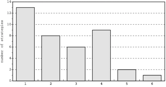
PROPERTY 3: Strategies contribute 7 tokens to the public activity in the final period(s).
Thirty-nine of the 50 strategies prescribe contributing 7 tokens to the public activity in one or more final periods, after having behaved according to different decision rules in the previous periods. We consider a strategy’s end phase to be all final periods in which it contributes 7 tokens. Figure 3 sums up the length of the 39 observed end phases. It shows the frequencies with which end phases of each length occur. The maximal length is 6 periods; the median is 2 periods.
PROPERTY 4: Strategies do not contribute fewer than 7 tokens.
Thirty-two of the 50 strategies would never make decisions below 7. If they use decision rules which are based on previous observations and potentially prescribe decisions below 7, they add additional rules to prevent this from occurring.
PROPERTY 5: Closed loop strategies are contingent on the last period or the last two periods.
Closed loop strategies consider previous decision rounds. Twenty-five of the 44 closed loop strategies are contingent on the previous period only. Thirteen closed loop strategies consider the two previous periods, while 3 strategies consider all previous periods. Strategies make use of the observed average contribution of the other group members or the entire group, and of their own
previous contributions. Few strategies consider other variables, such as their previous payoff or self-defined variables.
PROPERTY 6: Strategies use ROUND UP
ROUND TRUNCATE
average contribution of the others (or the entire group)
in the previous period + α
with α∈ {-1,0,1,2,3}, as decision rules.
Thirty of the 44 closed loop strategies use decision rules which are based on the average contribution of the other players or the average contribution of the entire group in the previous period. Twenty-one strategies consider the contribution of the other players, 6 strategies consider the group contribution, and 3 strategies consider both. Since decisions can be made as integers only, the observed averages have to be rounded in some way. Twenty strategies use the standard ROUND function, 4 strategies use TRUNCATE, 4 strategies use ROUND UP, and 2 strategies use more than one of these functions. Furthermore, we observe that strategies add an integer
α∈ {-1,0,1,2,3} to the observed average contribution. The most frequently chosen value for α is 0 (14 strategies). Values of (-1,1,2,3) are used by (2,5,1,1) strategies. Twenty-two of the 30 strategies that apply this rule use a unique rule specification. One-half (11) of these strategies use either ROUND with a strictly positive α or ROUND UP with α = 0, and thus have a tendency to be generous. About a quarter (6) of the strategies with a unique specification employ ROUND and α = 0, and thus closely reciprocate the previous average contribution. The remaining quarter (5) of the strategies with a unique specification use either ROUND with a negative α or TUNCATE with α = 0, and thus contribute a little less than the others to the public activity. Fourteen of the 30 strategies with decision rules of this kind use the decision rule uniformly in the sense that they apply exactly the same rule in all situations that may arise. However, some of these strategies put a lower limit (7 tokens) and/or an upper limit (an amount below 20 tokens) on their decisions.
These six properties describe a typical strategy.
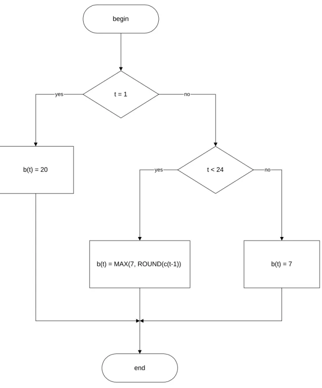
This typical strategy is closed loop with a phase structure. In the first period it contributes all of its endowment to the public activity. In an end phase it contributes 7 tokens. In the main phase it makes contributions between 7 and 20 tokens, using a decision rule as described by Property 6.
entire token endowment to the public good in the first period. It has an end phase of 2 periods. Its unique decision rule in the main phase prescribes reciprocating the average contribution of the others in the previous period, rounded to the nearest integer. It never contributes fewer than 7 tokens.
Let me mention three other properties found among the submitted strategies which are, however, not typical:
(1) Nine of the closed loop strategies put upper limits on their decisions. Six of them never contribute more than 19 tokens to the public activity, 2 strategies never contribute more than 18, and 1 strategy never contributes more than 13.
(2) Five closed loop strategies occasionally try to stimulate cooperation by contributing all of their endowment to the public activity. One strategy uses a random draw in each period to decide whether to stimulate cooperation or not, while 4 strategies (may) stimulate cooperation in one or two predetermined periods.
(3) Three strategies use random numbers in their decision rules.
Tables (a), (b), and (c) in Appendix B give an overview of the properties of each of the 50 submitted strategies. The most important distinction is between open loop (6 strategies) and closed loop (44 strategies). The closed loop strategies are further classified as strategies that use decision rules as described by Property 6 (30 strategies) and as strategies that do not use decision rules of this type (14 strategies). Among the latter are 6 strategies that use fixed numbers as decision rules.
Given the similarity of the closed loop strategies, their success in the simulation does not differ much (Appendix A). The realized payoffs of most strategies are very close. However, the closed loop strategies clearly do better than the few open loop strategies, which can all be found in the lower half of the ranking list. The U-test allows us to reject the null hypothesis that open and closed loop strategies enjoy equal success at the 1 percent significance level (two-sided test).
4.2 Typicity Measures
Selten, Mitzkewitz, and Uhlich (1997) introduce measures of typicity for strategies and typical properties, for which Kuon (1993) gives a mathematical justification. The idea is that not only strategies differ in how typical they are but properties may do so too. The degree to which both strategies and properties are typical can be measured by weights called typicities. There is an interdependent relationship between the typicities of strategies and the typicities of properties. The typicity of a strategy should be the sum of the typicities of the strategy’s properties. At the same time, the typicity of a property should be proportional to the sum of the typicities of the strategies which have this property.
above and s = (s1 ... s50)T denote the typicities of the 50 strategies participating in the third simulation. Let A = (aij) be a 6x50-matrix with entries aij = 1 if strategy j has property I, and aij =
0 otherwise. Then, c and s are uniquely determined by the following equations: (4.1) c = αAs,
(4.2) s = ATc,
with ∑i=1..6ci = 1, AT being the transpose of A, and 1/α being the largest eigenvalue of AAT. In
Equation (4.1), multiplication by α is necessary to ensure normalization of the vector c.
We compute the vectors c and s using an algorithm presented by Kuon (1993). The vector c is equal to
c = (0.19443, 0.14221, 0.17956, 0.14738, 0.19348, 0.14259).
Thus, we can order the properties according to their typicities. (1) Property 1 (closed loop structure) has the highest typicity and, thus, is the most typical property. (2) Property 5 (contingency on at most the last two periods) has the second highest typicity. The further ordering is (3) Property 3 (contribution of 7 tokens in an end phase), (4) Property 4 (never contribute fewer than 7 tokens),(5) Property 6 (typical rule), and (6) Property 2 (initial contribution of the entire token endowment to the public good).
Ranking the strategies’ typicities, we find a positive correlation between the typicities and the strategies’ success in the simulation. The Spearman rank correlation coefficient is equal to 0.60. Thus, we may reject the null hypothesis of no correlation between typicity and success of a strategy at the 1 percent level (two-sided test). Such an observation has also been made by Selten, Mitzkewitz, and Uhlich (1997): the more typical a strategy, the more successful it tends to be.
4.3 Some Remarks about Strategy Modifications
The major strategy modifications from the first to the third simulation were the following. In the first simulation, 7 strategies played the dominant strategy of contributing 7 tokens to the public activity in each period, 3 strategies always contributed zero, and 1 strategy contributed 7 tokens in uneven periods and zero tokens in even periods. All but one of these strategies (a strategy always contributing zero tokens) had disappeared by the final simulation round. The open loop strategies which were submitted in the final simulation round contributed, with the one exception mentioned, more than 7 in at least some periods.
Fifteen participants submitted the same strategy for all three simulation rounds. When closed loop strategies were changed, they were often made slightly more complex. End phases were included and, if end phase length was changed, it was more often extended than reduced this
being in keeping with Selten and Stoecker (1986). Initial contributions were more often increased than decreased. Sometimes the additional restriction not to go below 7 was introduced. Similarly, upper limits below 20 were sometimes introduced, as well as occasional contribution of the entire endowment to stimulate cooperation.
The strategies that were submitted for the first simulation round also tend to satisfy the six typical properties presented in Section 4.1. They satisfy them to a lesser extent, however.
5. A model of reciprocating behavior
Based on the typical properties of the strategies submitted by subjects, we present a simple model of reciprocating behavior in the specific public good situation.
Assume a large population of players i, with i = 1,...,N. The players are randomly matched in groups of n players (n << N) to play infinitely many repetitions of the constituent public good game presented in Section 2 (where each player is endowed with e = 20 tokens and the dominant strategy solution prescribes that each player contribute r = 7 tokens to the public activity B). The decision rule of each player i is given by
(5.1) b t
S
MAX r MIN e ROUND b t n
for t for t i j i j i ( ) ( , ( , (( ( ) / ( )) ))) , = − − + = > ≠
∑
1 1 1 1 αwith αi∈ {-1,0,1}, and S ∈ {r,...,e}.
Thus, each player starts the game in period t = 1 contributing an amount S to the public good. From the second period on, the contribution of player i in period t, bi(t), is based on the average
contribution of the other players in his group in the previous period, Σj≠ibj(t-1)/(n-1). There are
players who exactly reciprocate the observed average contribution of the other players in the group, rounded to the nearest integer. They have αi = 0, and we call them exact reciprocators.
Other players base their contribution on the observed average contribution but give one token more than the rounded value. They have αi = 1, and we call them generous reciprocators. There
are also players who always give one token less than the rounded average contribution of the other players in the previous period. They have αi = -1, and we call them cautious reciprocators.
No player would contribute less than 7 or more than 20 tokens.
We assume that p = prob(αi = 1) is the probability that, if we pick from the population any player
i, he has αi = 1; q = prob(αi = 0) is the probability that, if we pick from the population any player
i, he has αi = 0; and 1-p-q = prob(αi = -1) is the probability that, if we pick from the population
any player i, he has αi = -1. Note that each player i has a fixed αi which does not change over time.
Equation (5.1) describes a dynamic system. For any given group of n players, the values for αi are
given, and thus the system is deterministic. We can calculate its average contribution level in the limit. Due to the truncation at r = 7 and at e = 20 and to the rounding, this is analytically not easy to handle. The limit contribution can very easily be found by simulation, though. For the whole population of subjects, the dynamic system is a random variable. Once we know the distribution of the αi values, we can calculate the expected value of the average contribution level in the
population in the limit.7
In our experiment, with n = 4, we observe the majority of strategies to set S = 20. Furthermore, we identify, among the 22 strategies which have an invariant specification of the typical decision rule, about one half as reciprocating generously, one quarter as reciprocating exactly, and another quarter as reciprocating cautiously (see Section 5, above). Thus we assume that in our population
p = prob(αi = 1) = 0.5,
q = prob(αi = 0) = 0.25,
1-p-q = prob(αi = -1)= 0.25.
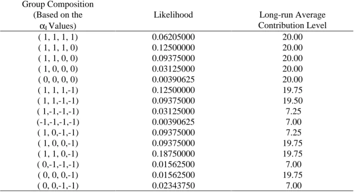
Table II shows the various possible group compositions (based on the αi values), the probability
of their occurrence and their contribution level in the limit. In the first column, the combination (1,1,0,-1), for example, means that the group is composed of two generous reciprocators, one exact reciprocator, and one cautious reciprocator. The second column displays the likelihood of such a combination. The likelihood of (1,1,0,-1), for example, is given by 12p2q(1-p-q). In the
third column, we find the average contribution level to which the respective group converges in the limit. The expected limit, or long-run average contribution level, in the entire population is 17.70. It is reached by the 40th period.
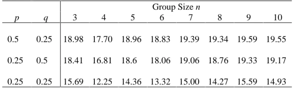
The long-run average contribution level depends on the initial contribution S, the (p,q)-distribution of the αi, and the group size n. Table III shows the limit contribution levels for initial
contributions varying from 7 to 20 (given p = 0.5, q = 0.25, and n = 4). The higher the initial contribution, the higher the long-run contribution level. This corresponds to an observation made by Keser and van Winden (2000).
Table IV compares long-run contribution levels for group sizes varying from 3 to 10 and for three different (p,q)-distributions. We cannot recognize a systematic group size effect. Note that Isaac, Walker, and Thomas (1984), Isaac and Walker (1988), and Isaac, Walker, and Williams (1994) also observe that group size has an unclear effect on the level of voluntary contributions to a public good. The comparison of the three (p, q)-distributions alone does not allow us to draw
7 Note that, in contrast to the experiments, this model considers an infinite time span. We present it in this way because it is convenient to consider the limit contribution level. Furthermore, the number of periods varies from one experiment to the other in the literature. The model can easily be modified for a finite number of periods, T, requiring that the system of Equations (5.1) holds for all t < T, and b(T) = r = 7.
general conclusions regarding the dependency of the contribution level on the distribution. But it yields support for the hypothesis that the smaller the proportion of cautious reciprocators and the higher the proportion of generous reciprocators in a population, the higher the contribution level tends to be. We suggest that treatment effects like higher contribution levels in public goods experiments with fixed groups than in experiments with changing group compositions (Croson 1996; Keser and van Winden 2000) can probably be explained as an effect on the proportions of the various types of subjects in a population. Keser and van Winden (2000) provide some evidence in favor of this explanation, observing a higher proportion of so-called cooperators in experiments with fixed groups than in experiments with changing group compositions.
6. Strategically planned versus spontaneous behavior
In this experiment, we observe strategically planned behavior. We have to take into account that it does not necessarily fully reflect spontaneous behavior. From experiments on dynamic duopoly situations (Keser 1992) we have some evidence that strategically planned and spontaneous behavior are qualitatively similar, but differ quantitatively. In the public good situation, qualitatively, the reciprocity aspect prevails both in spontaneous and strategically planned behavior. Keser and van Winden (2000), for example, give some evidence for reciprocity in spontaneous public good experiments.8 Reciprocity is defined there in a qualitative way. If a subject intends to change his decision from one period to the next, he changes it in the direction of the other group members’ average contribution in the previous period. This means that he increases his contribution if it was below the average of the others and decreases his contribution if it was above the average. Applying this definition of reciprocity to the data of Keser (1996), subjects significantly tend to behave in a reciprocal manner (two-sided binomial test, 1 percent level).
The specific quantitative model of reciprocating behavior presented in Section 5.1 appears not fully adequate for describing the spontaneous behavior observed in the experiment by Keser (1996). For each subject participating in the spontaneous game-playing experiment, we estimate the α-value under the assumption that he follows the decision rule (5.1). Of the 48 subjects, 27 can be characterized by an α which is significantly different from zero (t-test, 1 percent level). Fifteen subjects (31 percent of all subjects) show a negative α, while 12 subjects (25 percent of all subjects) show a positive α. The estimated α-values of these subjects lie between -8 and 9. This range is much larger than the one observed in the strategy experiment.9 Thus, although subjects’ behavior in the public good situation seems to be generally guided by the principle of
8 The importance of reciprocity motives has also been shown in many other experiments of various kinds. See, for example, Fehr, Gächter, and Kirchsteiger (1997) and the references given therein.
9 But, to translate this result into the model of reciprocating behavior, we determine p = 0.25 as the relative frequency of negative α-values, q = 0.44 as the frequency of α-values which are not significantly different from zero and 1-p-q = 0.31 as the relative frequency of positive α-values. The initial contribution observed in Keser (1996) is 10.5. Assuming an integer initial contribution of 10 (11), the long-run contribution level in our model is 11.27 (11.72), which is reached from period 31 (28) on. The average contribution level in Keser (1996) is 10.29.
reciprocity, the quantification appears different in spontaneous and strategically planned behavior.
Further evidence for reciprocity comes from regressions on random effect probit models. I ran regressions on the following one-way random probit models applied to the panel data set obtained from the experiments in Keser (1996):
Yit* = β0 + β1 D1Pit + β2 DL5Pit + β3 LAOCit + β4 (LAOC.DL5P)it + µi + vit,
where Yit* is the probability of playing the dominant strategy or the Pareto optimal solution, D1Pit is a dummy for the first period of the game, DL5Pit is a dummy for the last 5 periods of the game, LAOCit is the lagged average of the others’ contribution in the group, (LAOC.DL5P)it is a cross term variable, µi is a random individual effect, and vit is a random individual-time effect. Furthermore, i = 1,…,48, and t = 1,…,25.
We do not observe the probability that a subject will play the dominant strategy or the Pareto optimal solution, but instead observe whether the subject has actually played one of these strategies. Specifically, if we observe subject i at time t playing the dominant strategy, bit = 7, we define Yit = 1, and Yit = 0 otherwise. Similarly, for the Pareto optimal strategy, bit = 20 implies Yit = 1, and Yit = 0 otherwise. In the experiments, 27.08 percent of the individual decisions were the dominant strategy and 10.33 percent were the Pareto optimal solution.
Table V shows the regression results of these random probit models. For both strategies, we consider two specifications related to the conditional last period effect. In the first column, DL5P is directly included, affecting the level of the probability (i.e. changing the constant). In the second column, the cross term variable LAOC.DL5P is included, affecting the slope of the probability function in the contributions of the others.
Consider the first column of the regression results for the dominant strategy. The results show that in the first period of the game where the participants have no information about the contributions of the others in their group, the probability of playing the dominant strategy is low. In accordance with the findings on strategic behavior, the probability of playing the dominant strategy decreases with an increase in the average contribution of others in the group. The observed last period effect is also noticeable, as it sharply increases the probability of playing the dominant strategy.
In the second column of the regression results on the dominant strategy, the last period effect reduces the negative impact of the others’ contributions on the probability of playing the dominant strategy.
The results on the dominant strategy are reversed for the Pareto optimum. The estimated coefficients are all of opposite signs. For example, an increase in the others’ contribution increases the probability of choosing the Pareto optimal solution.
The rho-coefficient in all specifications is significantly important, confirming evidence of a random effect in our panel data. This justifies that the basic probit model would not have been appropriate.
All these results confirm the results on reciprocity in the strategy experiment.
The strategy experiment reveals that some subjects need the experience of some simulation rounds to learn that they have the opportunity to cooperate. The overall contribution level increases from one simulation round to the next. Analyzing the strategies participating in the final simulation round, we observe strategically planned behavior of highly experienced subjects. Contrary to this, spontaneous experiments on voluntary contributions to public goods are most often conducted with entirely or largely inexperienced subjects. Thus, subjects’ experience in playing the specific game might create an important difference between the spontaneous and strategic behavior. We observe that the time path of average contributions noted by Keser (1996) in spontaneous play is on the same level as that of the first simulation round of the present experiment. It would be very interesting to know whether in spontaneous experiments voluntary contributions to public goods also tend to increase with the subjects’ experience.
When comparing spontaneous play and strategically planned behavior, we should also take into consideration that in spontaneous play, aspects of behavior might become important that are immaterial in strategically planned behavior. For example, subjects’ spontaneous decision making might be influenced by negative feelings that possibly arise if low contribution by the other subjects is observed.
A striking difference between strategically planned and spontaneous behavior in the public good situation remains to be explained: in spontaneous play, we typically observe a downward trend of the average contribution to the public activity from the early to the late periods that does not show up in the strategy-based play. End game behavior, however, is observed both in spontaneous play (Keser 1996; Keser and van Winden 2000) and in strategically planned behavior.
7. Conclusion
Strategies reveal that there is a widespread willingness to cooperate. This willingness to cooperate is signaled in the first period. Then the typical strategy imitates or reciprocates the observed behavior in the group in the previous period. This imitation or reciprocation need not be to the exact point. Many strategies tend to be slightly more generous. Whatever the development of play, however, in the final few periods of the game, strategies play the dominant strategy solution. Even if a group showed cooperative behavior during the main phase, cooperation typically breaks down in the end.
7.1. Relation to Results of Previous Strategy Experiments
The results of this experiments are in keeping with those of earlier strategy experiments on the prisoners’ dilemma type of situations. A well-known early strategy experiment was run by Axelrod (1984). He asked subjects to design strategies to play a repeated prisoners’ dilemma game. The most successful strategy was tit-for-tat, a strategy which starts out cooperatively and then always imitates the behavior of the other strategy in the previous period. Selten, Mitzkewitz, and Uhlich (1997) and Keser (1992) used the strategy method of experimentation to examine behavior in asymmetric duopoly situations. While Selten, Mitzkewitz, and Uhlich (1997) examined a repeated Cournot duopoly, Keser (1992) examined a dynamic price-setting duopoly. In both studies, the submitted strategies typically reveal a phase structure and a system of case distinctions. Selten, Mitzkewitz, and Uhlich (1997) discovered a measure-for-measure principle: a typical strategy is designed to aim at a cooperative goal, which is individually specified based on equity considerations. The strategy reacts to the other player’s deviation from this goal in a reciprocating way.10 Thus, the typical strategy actively attempts to cooperate. In the public good experiment, the cooperative goal is, very obviously, the contribution of the entire token endowment to the public good.11 The reciprocating behavior is revealed in a simple orientation toward the average contribution of the other players in the previous period. That we can interpret it as an active attempt to cooperate becomes clear for two reasons. First, the willingness to cooperate is signaled in the first period when subjects tend to contribute their entire token endowment to the public good. Second, on average the value of α is positive.
We have replicated in this public good experiment the typical principles of strategic behavior in generalized prisoners’ dilemma situations. This experiment shows not only the robustness of these principles but also how they translate into the specific public good situation.
7.2. Policy Implications
This strategy experiment reveals that experienced subjects typically are willing to make higher voluntary contributions to public goods than predicted by economic theory. They do not contribute for reasons of being altruistic, kind, or confused. Rather they recognize the collective interest in having a high contribution level and actively attempt to achieve a high contribution level in the long-run interaction with others. Furthermore, we know that factors which reduce the
10 Reciprocity is often referred to in the experimental literature (e.g., Fehr, Gächter, and Kirchsteiger 1997). The reciprocity observed in the experiments discussed here is positive in that a subject cooperates as much as the others. Other experiments (e.g., Fehr and Gächter 1999) allow for and actually reveal negative reciprocity by the costly punishment of uncooperative others.
11
Keser and Gardner (1999) applied the strategy method of experimentation to examine behavior in an 8-player common pool resource game. In that experiment no cooperation was observed. The reasons seemed to be, first, the point of cooperation was not obvious to the subjects and, second, a subject expected not to have much impact as an individual on the behavior of the others. Evidence of the importance of an obvious cooperation point is also provided by Mason, Phillips and Nowell (1992) and Keser (2000). They observed more cooperative outcomes in symmetric than in asymmetric oligopoly experiments with spontaneous interaction.
social distance, such as mutual identification (Bohnet and Frey, 1995, 1999), and opportunities for communication and punishment (Ostrom, Gardner, and Walker 1992; Gächter and Fehr 1999; Fehr and Gächter 1999) increase the likelihood of cooperation. Given this positive news for voluntary cooperation, we should question in many public good situations in economic life whether government interventions are adequate or even necessary to increase efficiency. The voluntary contribution mechanism promises to work well in situations where the collective interest in voluntary contributions is obvious and where the social distance between the consumers of the public good is relatively small.
Andreoni (1993) shows that the public financing of a public good can have negative effects on the willingness to cooperate. He observed in a public good experiment that subjects who must pay a lump-sum tax contribute in total (voluntary contributions plus the tax) more than subjects who are not taxed. At the same time, however, taxes crowd out voluntary contributions by as much as 71 percent. This confirms the hypothesis by Frey (1997) that intrinsic motivation may be crowded out by extrinsic motivation.
As an example of successful funding by voluntary contributions, consider the case of the Public Broadcasting Service (PBS) in the United States. This is a private, nonprofit corporation whose members are America's public TV stations. It provides quality educational programs, products, and services for use in homes, schools, and workplaces. PBS is almost entirely financed by voluntary contributions. Its total operating revenue had grown to as much as $448 million by fiscal 1998. In contrast to this, public TV stations in Canada, which are mainly financed by taxes, seem to do less well in quality and budget. They would probably be better off with funding by voluntary contributions, as many Canadians are willing to make voluntary contributions to public TV, additionally to the taxes they pay. This shows in the contributions made by Canadians to PBS in the United States.12
12 See, for example, the list of underwriters to Vermont Public Television at URL
References
Anderson P.S., J.K. Goeree, and C.A. Holt (1998), "A Theoretical Analysis of Altruism and Decision Error in Public Goods Games," Journal of Public Economics, 70, 297-323. Andreoni J. (1988): "Why Free Ride?," Journal of Public Economics, 37, 291-304.
(1990): "Impure Altruism and Donations to Public Goods: A Theory of Warm Glow Giving," Economic Journal, 100, 464-477.
(1993): "An Experimental Test of the Public-goods Crowding-Out Hypothesis,"
American Economic Review, 83, 1317-1327.
(1995): "Cooperation in Public Goods Experiments: Kindness or Confusion," American
Economic Review, 85, 891-904.
Andreoni J., and J.H. Miller (1993): "Rational Cooperation in the Finitely Repeated Prisoner’s Dilemma: Experimental Evidence," Economic Journal, 103, 570-585.
Axelrod R. (1984): The Evolution of Cooperation. New York: Basic.
Barro R.J. (1974): "Are Government Bonds Net Wealth?," Journal of Political Economy, 82, 1095-1117.
Becker G.S. (1974): "A Theory of Social Interactions," Journal of Political Economy, 82, 1063-1093.
Benson B.L., and M.D. Faminow (1988): "The Impact of Experience on Prices and Profits in Experimental Duopoly Markets," Journal of Economic Behavior and Organization, 9, 345-365.
Bohnet I., and B.S. Frey (1995): "Ist Reden Silber und Schweigen Gold? Eine ökonomische Analyse," Zeitschrift für Wirtschafts- und Sozialwissenschaften (ZWS) 115, 169-209.
(1999): "The sound of silence in prisoner’s dilemma and dictator games," Journal of
Economic Behavior and Organization, 38, 43-57.
Cooper R., D.V. deJong, R. Forsythe, and T.W. Ross (1996): "Cooperation without Reputation: Experimental Evidence from Prisoner's Dilemma Games," Games and Economic
Behavior, 12, 187-218.
Croson R. (1996): "Partners and Strangers Revisited," Economics Letters, 53, 25-32.
Davis D.D., and C.A. Holt (1993): Experimental Economics. Princeton: Princeton University Press.
Fehr E., and S. Gächter (1999): "Cooperation and punishment in public goods experiments," forthcoming in: American Economic Review.
Fehr E., S. Gächter, and G. Kirchsteiger (1997): "Reciprocity as a Contract Enforcement Device: Experimental Evidence," Econometrica, 65, 833-860.
Frey B.S. (1997): Not just for the money: An economic theory of personal motivation. Cheltenham, UK: Edward Elgar Publishing.
Gächter S., A. Falk (1997): "Reputation or Reciprocity," Working Paper, University of Zürich. Gächter S., and E. Fehr (1999): "Collective action as a social exchange," Journal of Economic
Behavior and Organization, 39, 341-369.
Isaac R.M., J.M. Walker (1988): Group Size Effects in Public Goods Provision: The Voluntary Contribution Mechanism, Quarterly Journal of Economics, 103, 179-200.
Isaac R.M., J.M. Walker, and S.H. Thomas (1984): "Divergent Evidence on Free Riding: An Experimental Examination of Possible Explanations," Public Choice, 43, 113-149. Isaac R.M., J.M. Walker, and A.W. Williams (1994): "Group Size and the Voluntary Provision
of Public Goods," Journal of Public Economics, 54, 1-36.
Keser C. (1992): "Experimental Duopoly Markets with Demand Inertia: Game-Playing Experiments and the Strategy Method," Lecture Notes in Economics and Mathematical
Systems, 391. Berlin: Springer Verlag.
(1993): "Some Results of Experimental Duopoly Markets with Demand Inertia," Journal
of Industrial Economics, 41, 133-151.
(1996): "Voluntary Contributions to a Public Good when Partial Contribution is a Dominant Strategy," Economics Letters, 50, 359-366.
(2000): "Cooperation in Symmetric Duopolies with Demand Inertia," International
Journal of Industrial Organization, 18, 23-38.
Keser C. and R. Gardner (1999): "Strategic behavior of experienced subjects in a common pool resource game," International Journal of Game Theory, 28, 241-252.
Keser C., and F. van Winden (2000): "Conditional cooperation and voluntary contributions to public goods," Scandinavian Journal of Economics, 102, 23-39.
Kreps D.M., P. Milgrom, J. Roberts, and R. Wilson (1982): "Rational Cooperation in the Finitely Repeated Prisoners' Dilemma," Journal of Economic Theory, 27, 245-252.
Kuon B. (1993): "Measuring the Typicalness of Behavior," Mathematical Social Sciences, 26, 35-49.
Ledyard J. (1995): "Public Goods: A Survey of Experimental Research," in The Handbook of
Experimental Economics, ed. by A.E. Roth and J. Kagel. Princeton: Princeton
University Press.
Mason C.F., O.R. Phillips, and C. Nowell (1992): "Duopoly behavior in asymmetric markets: an experimental evaluation," Review of Economics and Statistics, 74, 662-669.
McKelvey R.D., and T.R. Palfrey (1992): "An Experimental Study of the Centipede Game,"
Palfrey T.R., and J.E. Prisbrey (1998): "Anomalous Behavior in Public Goods Experiments: How Much and Why?," American Economic Review, 87, 829-846.
Selten R. (1967): "Die Strategiemethode zur Erforschung des eingeschränkt rationalen Verhaltens im Rahmen eines Oligopolexperiments," in Beiträge zur experimentellen
Wirtschaftsforschung, ed. by H. Sauermann. Tübingen: J.C.B. Mohr.
Selten R., M. Mitzkewitz, and G. Uhlich (1997): "Duopoly Strategies Programmed by Experienced Players," Econometrica, 65, 517-555.
Selten R., and R. Stoecker (1986): "End Behavior in Finite Prisoner's Dilemma Supergames,"
Journal of Economic Behavior and Organizations, 7, 47-70.
Sefton M., and R. Steinberg (1996): "Reward Structures in Public Good Experiments," Journal
of Public Economics, 61, 263-287.
Stoecker R. (1980): Experimentelle Untersuchung des Entscheidungsverhaltens im
Bertrand-Oligopol. Bielefeld: Pfeffer.
(1983): "Das erlernte Schlußverhalteneine experimentelle Untersuchung," Zeitschrift
0 1 2 3 4 5 6 7 8 9 10 11 12 13 14 15 16 17 18 19 20 1 2 3 4 5 6 7 8 9 10 11 12 13 14 15 16 17 18 19 20 21 22 23 24 25 period
average contribution to activity B
first simulation second simulation third simulation
FIGURE 1 Time paths of average contributions to the public activity B in the 3 simulation rounds.
0 1 2 3 4 5 6 7 8 9 10 11 12 13 14 15 16 17 18 19 20 0 5 10 15 20 25 30 35 number of strategies 0 1 2 3 4 5 6 7 8 9 10 11 12 13 14 15 16 17 18 19 20 initial contribution
FIGURE 2 Initial contributions to the public activity B.
(We consider 48 strategies participating in the third simulation round, and exclude from consideration 2 strategies which choose random numbers in the first period.)
1 2 3 4 5 6 0 2 4 6 8 10 12 14 number of strategies 1 2 3 4 5 6
length of end phase (number of periods)
FIGURE 3 Length of end phases of the 39 strategies that specify an end phase in the final simulation round.
b(t) = 20 t = 1 t < 24 b(t) = 7 b(t) = MAX(7, ROUND(c(t-1)) no no yes yes end begin
FIGURE 4 Flow chart of a typical strategy to be called up in each period t
(The variable b(t) denotes the own contribution to activity B in period t, and c(t-1) is the average contribution of the other players in period t-1.)
TABLE I
Payoff from Tokens Used for Activity A
Token Payoff from that
Token (in ExCU)
Cumulative Payoff from All Tokens Used
in A (in ExCU) 1st 2nd 3rd 4th 5th 6th 7th 8th 9th 10th 11th 12th 13th 14th 15th 16th 17th 18th 19th 20th 40 38 36 34 32 30 28 26 24 22 20 18 16 14 12 10 8 6 4 2 40 78 114 148 180 210 238 264 288 310 330 348 364 378 390 400 408 414 418 420
TABLE II
Likelihood and Long-run Average Contribution Level for Each Possible Group Composition (Experiment Conditions)
Group Composition (Based on the
αI Values)
Likelihood Long-run Average
Contribution Level ( 1, 1, 1, 1) 0.06205000 20.00 ( 1, 1, 1, 0) 0.12500000 20.00 ( 1, 1, 0, 0) 0.09375000 20.00 ( 1, 0, 0, 0) 0.03125000 20.00 ( 0, 0, 0, 0) 0.00390625 20.00 ( 1, 1, 1,-1) 0.12500000 19.75 ( 1, 1,-1,-1) 0.09375000 19.50 ( 1,-1,-1,-1) 0.03125000 7.25 (-1,-1,-1,-1) 0.00390625 7.00 ( 1, 0,-1,-1) 0.09375000 7.25 ( 1, 0, 0,-1) 0.09375000 19.75 ( 1, 1, 0,-1) 0.18750000 19.75 ( 0,-1,-1,-1) 0.01562500 7.00 ( 0, 0, 0,-1) 0.01562500 19.75 ( 0, 0,-1,-1) 0.02343750 7.00 TABLE III
Long-run Population Contribution Levels for Varying Initial Contributions (p = 0.5, q = 0.25, group Size n = 4)
Initial Contribution b(1)
7 8 9 10 11 12 13 14 15 16 17 18 19 20
TABLE IV
Long-run Population Contribution Levels for Varying Distributions(p,q) and Group Sizes (Initial Contribution of 20) Group Size n p q 3 4 5 6 7 8 9 10 0.5 0.25 18.98 17.70 18.96 18.83 19.39 19.34 19.59 19.55 0.25 0.5 18.41 16.81 18.6 18.06 19.06 18.76 19.33 19.17 0.25 0.25 15.69 12.25 14.36 13.32 15.00 14.27 15.59 14.93 TABLE V
Regression Results of Random Probit Models (t-values)
Variable Dominant Strategy Pareto Optimal Solution
Constant 0.04109 (0.191) 0.1174 (0.575) -2.642 (-9.93) -2.727 (-10.33) D1P -1.097 (-2.63) -1.185 (-2.805) 0.6250 (1.83) 0.7236 (2.15) DL5P 0.4201 (4.18) -0.6523 (-2.74) LAOC -0.1379 (-7.35) -0.1471 (-7.94) 0.06198 (3.89) 0.06979 (4.27) LAOC.DL5P 0.04659 (3.95) -0.05368 (-2.09) ρ(µ,v) 0.6366 (20.11) 0.6335 (20.44) 0.4586 (5.24) 0.4518 (5.10)
APPENDIX A – Ranking of Average Profits in the Third Simulation Round (230300 Plays in Total, 18424 Plays per Strategy)
Rank Profit ExCU Profit US $ Strategy No. : Name
1 26425.69 264.26 32 : Justus Haucap
2 26389.41 263.89 56 : Picard & Wibaut
3 26384.52 263.85 57 : Campbell Macdonald 4 26384.02 263.84 43 : Bentley MacLeod 5 26379.35 263.79 53 : David Moffat 6 26368.66 263.69 47 : Anonymous 7 26353.19 263.53 19 : Karl-Martin Ehrhart 8 26343.30 263.43 40 : Daniel Borowski 9 26341.35 263.41 9 : James Walker 10 26332.19 263.32 4 : Otto Perdeck 11 26331.62 263.32 51 : Evelyn Otto 12 26329.10 263.29 52 : Erwin Amann 13 26327.06 263.27 1 : Nick Feltovich 14 26325.87 263.26 30 : Bruce Lyons 15 26317.60 263.18 20 : Rachel Croson 16 26308.72 263.09 33 : Jens Barmbold 17 26280.65 262.81 11 : Bjoern Ebbesen 18 26280.15 262.80 34 : Hildegard Foerster
19 26270.25 262.70 42 : Andreas Flache & Rene Torenvlied
20 26267.14 262.67 27 : 'MrKind' 21 26261.23 262.61 7 : Jozsef Sakovics 22 26255.00 262.55 3 : Joep Sonnemans 23 26249.63 262.50 26 : Arno Riedl 24 26247.62 262.48 12 : Olaf Dalchow 25 26217.67 262.18 44 : Joerg Naeve 26 26210.96 262.11 13 : Rob Eken 27 26187.38 261.87 41 : Burkhard Hehenkamp 28 26186.90 261.87 8 : Robert Sugden 29 26180.08 261.80 39 : Jeroen Jansen
30 26177.75 261.78 46 : Weber & Eisenberger
31 26169.38 261.69 50 : Hans Henning
32 26159.12 261.59 55 : Malnero & Vannetelbosch
33 26135.33 261.35 45 : Anonymous 34 26049.27 260.49 6 : Harald Wiese 35 26035.07 260.35 36 : Bodo Schirra 36 26026.38 260.26 24 : Steven Backerman 37 26013.06 260.13 31 : Gregory K. Dow 38 25960.35 259.60 48 : Rainer Overbeck 39 25945.44 259.45 10 : Theo Offerman 40 25866.08 258.66 49 : Christiane Oelschlae 41 25780.26 257.80 28 : Axel Ostman 42 25667.63 256.68 37 : Anonymous
43 25590.82 255.91 58 : Juergen von Hagen
44 25278.51 252.79 38 : Albert Hart 45 25176.96 251.77 29 : 'UCP-Team ' 46 25122.45 251.22 35 : Lars P. Feld 47 24962.27 249.62 5 : Roy Gardner 48 24585.80 245.86 2 : Joergen Wit 49 21798.61 217.99 25 : Stephan Levy 50 20406.95 204.07 22 : Anonymous
APPENDIX B (a)
Properties of the 30 Closed Loop Strategies which Use Decision Rules as Described by Property 6 Typical Rule No. b(1) End Phase Length Cond. upon Max. ≥ 7 Yes No Up Round Trunc Others Group α Uniform Upper Limit < 20 Coop. Stim. Ran-dom 19 20 2 t-1 Y T O 0 Y 20 20 1 t-1 Y U O 0 Y 1 20 1 t-1 Y T O 0 Y 30 20 1 t-1 Y R O 0 Y 12 20 1 t-1 N R O 0 Y 19 55 20 4 t-1 Y R O -1 Y 24 12 4 t-1 Y R O -1 Y 53 20 4 t-1 N R O 1 Y Y 46 19 1 t-1 N R O 1 Y 33 20 1 t-1 Y R O 1 Y Y 27 20 - t-1 N R O 2 Y 9 20 - t-1 Y T G 0 Y 57 20 1 t-1 N U O 0 Y 13 34 20 1 t-2 N R O 0 Y 39 17 1 t-1 Y T* O Var. N 47 20 4 t-1 N R O/G 0 N Y 32 20 1 t-1 Y U O/G 0 N 3 12 3 t-2 N R O 1 N 19 40 20 5 t-1 Y R G 0 N Y 36 7 1 t-1 N R G 1 N 4 18 6 t-1 N R O 3 N 51 19 3 t-2 Y R G Var. N 19 10 17 3 t-2 N R O Var. N 26 20 - t-2 N R O Var. N 50 13-17 2 t-1 Y Var. O/G 0 N 11 20 1 All Y T O Var. N 52 18 4 t-2 Y R O 0 N 18 28 14 - t-2 N U G 0 N 19 41 14 3 t-3 Y R O Var. N 19 7 12 2 t-2 Y R G Var. N 19 *
APPENDIX B(b)
Properties of the 14 Closed Loop Strategies which Do Not Use Typical Decision Rules
No. b(1) End Phase Length Cond. upon Max. ≥ 7 Yes No Decisions, if Only Predetermined Values Upper Limit < 20 Coop. Stim. Random 8 20 - t-1 Y Y 42 20 2 t-2 Y 44 20 2 t-2 Y Y Y 37 18 - t-2 N 58 7 4 t-1 Y 35 15 - t-9 N Y 43 20 4 t-2 Y 56 20 3 All Y 48 20 2 All N 0,7,20 13 20 - t-1 Y 7,10,15,20 6 20 2 t-2 Y 7,20 31 20 - t-3 Y 7,20 29 20 1 t-1 Y 7,20 25 20 - t-1 N 0,20 APPENDIX B(c)
Properties of the 6 Open Loop Strategies
No. b(1) End Phase Length ≥ 7 Yes No Decisions Upper Limit < 20 Coop. Stim. Random 38 20 2 Y Random (7-20) Y 2 7-13 5 Y Random (7-13) 13 Y 49 20 1 Y Dependent on t: 20,...,7 45 20 4 Y Always 20 22 0 - N Always 0 0 5 10 3 Y Dependent on t: 10,20