109
Tax Capacity and Tax Effort of ALGERIA from 1981 to 2014 Dr. Toufik HADJMAOUI 1, Dr. Hanane BENATEK 2
1 Researcher Professor at University of Saida, Algeria E-mail: hadjmaoui_toufik@yahoo.fr
2 Researcher Professor at University of Mascara, Algeria E-mail: behanane_dz2002@yahoo.fr
Received: 01/02/2018 Accepted: 20/06/2018 Published: 30/06/2018
Abstract:
The purpose of the present study is determine the principal determinants of taxes Capacity, then measure the tax effort of Algeria; by employing time-series econometric techniques over the period 1981-2014.
The Results indicate that tax effort index is relatively stable about number one (1), that is the case in which the tax actual revenue equal potential tax revenue (Potentiel) which indicates that Algeria can not collect more tax revenue in the current economic situation.
Keywords: Tax capacity, Tax effort, Tax revenue. JEL classification codes: H20, E62, O23
__________________________________
110 1. INTRODUCTION:
Algeria has made significant progress in its development; this improvement is due to the high public expenditure level inrecent years. Statistics indicate in this context that the human development index of Algeria (HDI) moved from 0.577 in 1990 to0.745in 2015; Algeria, which is classified in the worldranked83among188 countries.
0.577 to 0.745, an increase of 29.1 percent. Table a reviews Algeria’s progress in each of the HDI indicators. Between 1990 and 2015, Algeria’s life expectancy at birth increased by 8.3 years, mean years of schooling increased by 4.2 years and expected years of schooling increased by 4.8 years. Algeria’s GNI per capita increased by about 36.8 percent between 1990 and 2015. (HDR, 2016)
In order to stay at the same direction, it is required to generate additional tax revenue to cover the increased public expenditure. But the question that arises are the Algerian economy is able to bear the additional tax burden? This is what we are trying to answer in this paper by dividing this work to:
a) Taxable Capacity and Tax Effort: Empirical Analysis. b) Model Specification and Methodology.
c) Tax Capacity: Model estimation results. d) Tax effort: Estimation Results.
e) Conclusion and recommendations.
2. Taxable Capacity and Tax Effort: Empirical Analysis Definitions Of Taxable Capacity And Tax Effort
According to economic literature, the taxable capacity and the tax effort of countries have been estimated using regression analysis, focusing on possible determinants of taxes.
While tax capacity represents the maximum tax revenue that could be collected in a country given its economic, social, institutional, and demographic characteristics, potential tax collection represents the maximum revenue that could be obtained through the law tax system. Tax gap is the difference between this potential tax collection and the actual revenue, which is a function of tax capacity and the extent to which, by tax
111
laws and administration, a society wishes to mobilize resources for public use. (Pessino, 2010)
Tax effortis defined as an index of the ratio between the share of the actual tax collection in grossdomestic product and the predicted taxable capacity. A “high tax effort” is the case when a tax effort index is above 1, implying that the country well utilizes its tax base to increase tax revenues (Stotsky, et al., 1997). A “low tax effort” is the case when a tax effort index is below 1, indicating that the country may have relatively substantial scope or potential to raise tax revenues. (Minh Le, Moreno-Dodson, & Bayraktar, 2012).
The use of tax effort and actual tax collection benchmarks allows the ranking of countries into four different groups:
- low tax collection, low tax effort; - high tax collection, high tax effort; - low tax collection, high tax effort; - high tax collection, low tax effort. -
3. Model Specification And Methodology:
The empirical specifications used in the paper consist of possible determinants of tax revenue and total fiscal revenue as a share of GDP:
(TAX/GDP)t = α + βXt+ εt… … … (1)
Where:
α: Intercept ε: error term
The dependent variable; TAX/GDP: Total Tax Revenue as a Share of
Gross Domestic Product.
Generally, it explain the actual income tax rate to GDP as a measure of tax effort that used as a basis for comparing the tax systems between countries, but the use of this ratio is reasonable to compare the tax performance of a group of countries that have the same economic structure with the same level of income.
For this, the use of this ratio comparison, the effectiveness of the mobilization of incomes between countries that their incomes are different,
112
it may give us a completely distorted picture because of differences in economic structures, demographic trends. As a result, many economists who are interested in taxes to deal with this problem through an economitric studies to assess the determinants of income tax and determine the effect of each variable on the tax capacity of any country (Minh Le, Moreno-Dodson, & Bayraktar, 2012), and this is what we are going to treat in this study.
The explanatory variables Xt:
Employed in the Basic model follow those used in the conventional tax effort literature. The explanatory variablesserve as possible fiscal proxies for possible tax bases and other factors that might affect a country's ability toraise tax revenues.
Xt=LGdppct, Inft, Agrict, Tradet, Manft, Urbant, Shadowt, Inst, Oilt, Dept
LGdppct: Per capita GDP was expressed in logarithm.
AGRIC: agriculture value added in percentage of GDP. MANF: manufacturing value added in percentage of GDP. INF: the rate of consumer price inflation.
TRAD: measures trade openness (exports plus imports in percentage of GDP).
URBAN: the share of the urban population in total population. DEPT: External debt in percentage of GDP.
OIL: hydrocarbon export as a percent of total exports.
SHADOW is a measure of shadow economic activity, taken in percent of GDP.
LGDPPC:
Per capita GDP is a proxy for the level of development of a country. A higher level of development goes together with a higher capacity to pay and collect taxes, as well as a higher relative demand for income elastic public goods and services (Chelliah, 1971; Bahl 1971). In general, it is expected to be positively correlated between the level of per capita income and the level of tax effort. (Bird, Martinez-Vazquez, & Torgler, 2004)
113
The presence of AGRIC in equation is dictated by general (administrative and political economy) difficulties of taxing agriculture and the intentions of many governments to either provide tax exemptions or subsidies (or both). The presence of a large rural sector also reduces the demand for government services, since many public sector activities are city-based (Hamid, Davoodi, & David, 2007) Stotsky and WoldeMariam (1997) and Leuhold (1991) investigated determinants of the share of tax revenue in GDP for African countries using panelresearch methodology. The results showed that the share of agriculture in GDP negatively influence the share of tax revenue in GDP. (murunga, Muriithi, & kiira, 2016).
MANF:
We considered the manufacturing value added in percentage of GDP as the approximate indicators of the stage of development, then, it is expected that this indicator have positive effect on tax capacity. (Tanzi, 1981)
Inflation:
We define inflation as an approximate indicator for Macro-economic Policies. Having a high inflation will have effectiveness on tax revenues due to its effect on consuming and investment, it also has a negative effect on the ability of contributor’s participation, thus, itis expected that this indicator have negative effect on tax capacity.
Urban:
Urban population refers to people living in urban areas.If this ratio is high, it means that goods and public services having a high demand which will lead to an approximate tax revenue, in addition to facilitate taxation on urban zones by the tax administration as a result, itis expected that this indicator have positive effect on tax capacity. (Shin, 1969)
TRADE:
We include TRADEin the regressions and expect it to have a positive impact on tax collection. Is known as the international trade sector and private imports of sectors characterized by easily collected, they are considered the most important fiscal resources for developing countries.
114
Lutfunnahar (2007) identified the determinants of tax share and revenue performance for Bangladesh along with 10 other developing countries for the 15 yearsthrough a panel data analysis. The results obtained suggest international trade to be significantly determinants of tax efforts.Mahdavi (2008) used the advanced estimation techniques with an unbalanced panel data for 43 DCs over the period 1973-2002. His results showed that trade sector share had a positive effect. (Imran & Farzana, 2010)
Dept:
Theshare of external debt in GDP show us the dependence of a certain country from the whole foreign aid, the rise of this ratio means a weak tendency towards internal resource mobilization , therefore it is expected that for this variable negative impact on tax capacity, and this was confirmed by both Gupta and Al, through a study carried out by of a sample of 107 countries that have an external debt for the period between 1970 and 2000, concluded that the the rise of foreign debt lead to the decrease of tax revenue for countries who have debts.
Shadow:
The economy of developing countries were charactrized by a parallel economy (hidden economy), with a different size from one country to another.
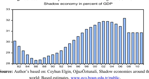
Algeria is one of those countries that suffer from this phenomen and its implications. If the hidden economy has a large share in GDP, it would negatively affects the size of the tax revenue because of the unwillingness of the citizen to pay the tax and decrease the spirit of tax contribution.Pyle (1989) points out that one of the implications of the existence of the underground economy is that some income goes untaxed and also certain indirect taxes are also evaded. (Rasheed, 2006)
The following figure shows us the importance of the shadow economy relative to official GDP in Algeria for the period between1981 and 2011:
115
Fig. 1. Shadow Economy in Percent of GDP In Algeria 1981-2011
28 29 30 31 32 33 82 84 86 88 90 92 94 96 98 00 02 04 06 08 10
Shadow economy in percent of GDP
Source: Author’s based on: Ceyhun Elgin, OĝuzÖztunali, Shadow economies around the
world: Based estimates. www.eco.boun-edu.tr/public.
The difference in the size of tax evasion and the shadow economy from one country to anotherand which does not appear in full in the gross domestic product, the use of this rate in the comparison between that different countries gave us an unclear image and confusion. (L'OCDE, 2000)
As already noted above, the effect of variation from one country to
another in the nature of social security revenues.
The difference in measurement of GDP.
Absence of a reference rate can be invoked in comparison with the
exception of Colin Clark at estimated at 25%.
The difference in the institutional structures from one country to
another could have huge implications on tax effort rate, without having a significant impact on the burden that could be left behind the tax. As a difference from one country to another in the size of the amounts paid as a tax by the same public sector and in the combination of subsidies and tax expenditures (exemptions, reductions and tax credit). (l’OCDE, 2001)
Oil:
In this equation we involved oil exports part in total exports in order to explain how much the Algerian economy dependency on petroleum tax
116
revenues, and we expect the ratio of oil exports will have a positive effect on tax capacity.
3.1. Data Description:
All the data used in this study were obtained from the IMF (International Financial Statistics), World Bank database, Central Bank of Algeria. Annual data series which covers the period 1980-2014 was used to estimate the parameters of the model.
Table 1. Descriptive Statistics
Variables Mean Std. Dev Min Max
Y: Tax/GDP 33.27 5.94 23.7 45.77 LGdppct 8.56 0.27 8.1 9.04 Agrict 10.02 1.74 6.92 13.04 Manft 9.77 3.31 4.63 15.71 Trade 54.86 10.13 32.68 71.92 Inft 9.94 9.00 0.34 31.67 Urbant 57.87 8.73 44.0 73.0 Deptt 38.65 22.12 3.04 79.14 Shadowt 30.28 1.27 28.32 32.2 Oilt 96.85 1.16 93.41 98.35
Source: Author’s calculation 3.2. Stationarity test.
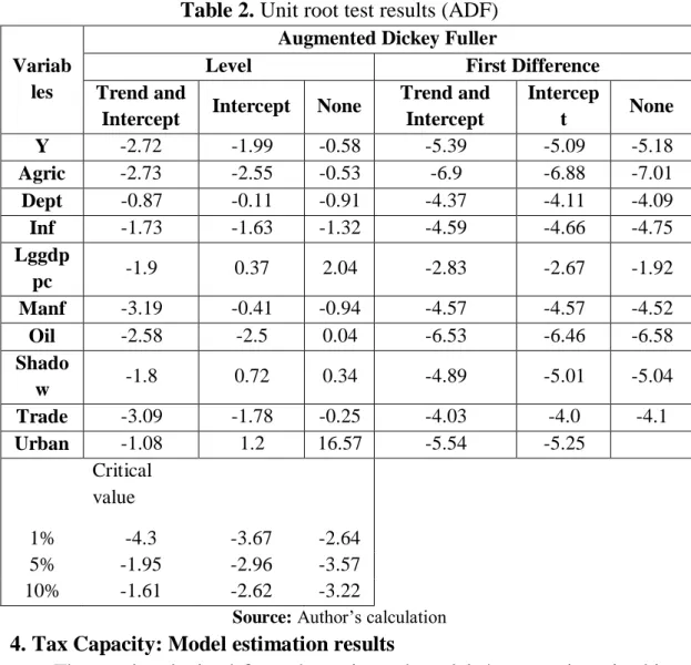
As an initial step stationarity tests must be performed for each of the variables. Although, there have been a variety of proposed methods for implementing stationarity tests, in this study, the Augmented Dickey-Fuller (ADF) test (Dickey and Fuller, 1979) was employed.
Table 2reports the results of the ADF test both in levels and first differences. The appropriate lag lengths are selected according to the Schwartz info criterion. The ADF statistic suggests that all variables are stationary in their first differences.
117
Table 2. Unit root test results (ADF) Variab
les
Augmented Dickey Fuller
Level First Difference
Trend and
Intercept Intercept None
Trend and Intercept Intercep t None Y -2.72 -1.99 -0.58 -5.39 -5.09 -5.18 Agric -2.73 -2.55 -0.53 -6.9 -6.88 -7.01 Dept -0.87 -0.11 -0.91 -4.37 -4.11 -4.09 Inf -1.73 -1.63 -1.32 -4.59 -4.66 -4.75 Lggdp pc -1.9 0.37 2.04 -2.83 -2.67 -1.92 Manf -3.19 -0.41 -0.94 -4.57 -4.57 -4.52 Oil -2.58 -2.5 0.04 -6.53 -6.46 -6.58 Shado w -1.8 0.72 0.34 -4.89 -5.01 -5.04 Trade -3.09 -1.78 -0.25 -4.03 -4.0 -4.1 Urban -1.08 1.2 16.57 -5.54 -5.25 Critical value 1% -4.3 -3.67 -2.64 5% -1.95 -2.96 -3.57 10% -1.61 -2.62 -3.22
Source: Author’s calculation 4. Tax Capacity: Model estimation results
The results obtained from the estimated model that are given in this equation:
Y = 38.75 – 2.3 8 AGRIC – 0.0 8 DEPT + 0.02INF + 4.11LGGDPPC – 0.5Manf (0.16) (-4.06) (-0.9) (0.2) (0.14) (0.71) - 0.3 OIL + 1.58SHADOW – 0.0 5 TRADE – 0.4 4 URBAN
(-0.37) (0.95) (-0.029) (-0.48)
(.) t. Student
𝑅2 = 0.83 𝑅̅2 0.75 𝑃𝑟𝑜𝑏(𝐹. 𝑆𝑡𝑎𝑡𝑖𝑠𝑡𝑖𝑐) = 0.000 𝐷𝑊 = 2.29
We Notes from the estimated relationship that all explanatory variables parameters are not significantly different from zero, except the
118
share of agriculture parameter, and this is what might be considered an indicator of the existence of a multicollinearity between the independent variables and is against with the assumptions which is upon the method of ordinary least squares, because this presence of such correlation between the explanatory variables entail that the estimated relationship parameters may show signs contrary to what is expected as well as, therefore, we find that the critical Probabilities exceed 0.05. (Bourbonnais, 2011)
4.1. Test for the Existence of Multicollinearity Problem
For the detection of the existence and severity of multicollinearity in this function, we rely on Farrar-Glauber test represented in the following test steps:
- Calculate the determinant matrix correlation coefficients between the independent variables, if the value of this determinant close to zero, it prooves the existence of multicollinearity problem.
- Test of the following hypothesis:
H0: D=1: No multicollinearity exists (explanatory variables are orthogonal)
H1: D<1: Multicollinearity exists (explanatory variables are not orthogonal)
To test the hypotheses are statistically Farrar-Glauber calculated using the following formula: (Bourbonnais, 2011)
𝜒𝑐𝑎𝑙2 = − [𝑛 − 1 −1
6(2𝑘 + 5)] − 𝑙𝑛𝐷
n: Sample size
K: Number of explanatory variables in the model.
D: Determinant matrix of correlation coefficients between the independent variables.
If the statistical Farrar-Glauber greater than the chi-squared statistic degree of freedom ½ * k (k + 1) This indicates the presence of Multicolinarity. And relying on Excel program we have calculed the determinant matrix of correlation coefficients between the independent variables D = 0.0000009737. We note that the determinant value close to zero and is an indication of the presence of Multicolinearityand to verify, we calculate the statistical Farrar-Glauber and comparing the chi-squared statistic..
119
Conclusion: Since𝜒𝑐𝑎𝑙2 = 362.19 is greater than𝜒2 = 1.51, we reject H 0.
Therefore, it is reasonable to conclude that there is a presence of multicollinearity problem.
4.2. All Possible Regression Method of Selection of the Best Regression Model:
Reaching the conclusion that the existence of a multicollinearity means that there is some independent variables that have the same effect on the dependent variable, therefore, they must not appear in the model that requires choosing the perfect model that includes independent variables which have the following conditions: (Bourbonnais, 2011)
- Variables that have a strong correlation with the dependent variable. - Variables that have a least correlated with each other.
To choose the ideal model we follow All possible regressions procedure because it is the best one (Bourbonnais, 2011) , This method gave us a permission to estimate all possible regression and select the best one , Although this procedure requires many calculations, therefore, the number of different regression equations estimated to 29-1=511, we
can clearly from estimating regression equations that in all cases cannot estimate asignificant regression equation that include more than two variables, and the reason for that , is due to the strong multicollinearity between the different explanatory variables. After the exclusion of all models that include at least a variable that is not significant (except intercept) or which include parameters of variables that have a wrong signals ,we selected the best models from the remaining models, which achieved the lowest value for the standard Akaike and Schwarz and summarized in the following table:
120
Table 3. Tax Capacity: Determinants of Taxable Capacity Independent
Variables
Dependent Variable: Tax revenue/GDP
Model (1) Model (2) Model (3)
Intercept 63.35 (20.51) -189.88 (-3.17) 19.93 (3.9) Agriculture/GDP -3.00 (-9.88) Oil 2.13 (3.35) Trade (% of GDP) 0.32 (4.35) 0.31 (4.06) Deptt -0.1 (-2.86) R2=0.77 F.Stat=97.62 DW=1.86 R2=0.66 F.Stat=26.65 DW=1.76 R2=0.63 F.Stat=23.52 DW=1.33 Source: Author’s calculation(.) t.student
The results of the first model indicate, and as we expected, the presence of a strong negative relationship and which have significant statistically between the share of agriculture and income tax,it is reached by both Junet. G. Stosky and A. Woldmariam 1997 and Chelliah, Kelly, Bass 1974. This negative relationship is due to the strengthening of the agricultural sector either by tax exemptions or subsidies granted by the government, or both, in addition to the presence of a large rural sector resulted a low demand from government services because most public sector activities centered in the cities V. Tanzi 1992.
The results of the second model indicate a strong positive relationship and significant statistically between the share of oil exports and tax revenue, this result is consistent largely associated with the Algerian economy structure and strongly linked to the composition of the oil revenue. The same model also suggests a positive relationship between the degree of economic openness and tax revenue. That was reached by M. Piaccastelli. The higher the country's commercial dealings with the outside world is the higher rise in tax revenues, because these transactions and as
121
agreed in the various tax studies constitute a tax basis and which characterized by an easy collection of taxes compared with the transactions inside especially for developing countries, Moreover, the third model results shows, and as it was expected, the presence of a negative and significant relationship between external debt quota and tax revenue, the external debt ratio as a GDP is considered as an indicator of the level of subordination of the country to foreign aid, as a result, the rise of this ratio is often translated to a weak tendencies towards the mobilization of domestic resources.
5. Tax effort: Estimation Results
Based on the results of the estimated regression equations, that express the potential tax ratio to GDP, andwhich measures the potential taxes of Algeria, we calculated tax effort indicator as shown in the following table:
Table 5. Tax Effort Index Tax Effort Model (1) Model (2) Model (3) Tax Effort Model (1) Model (2) Model (3) 1981 0.978 0.876 0.966 1998 1.036 0.888 0.97 1982 1.167 1.176 1.288 1999 1.043 0.876 0.936 1983 0.998 1.089 1.204 2000 1.032 1.019 1.093 1984 0.897 1.048 1.093 2001 1.023 0.955 0.975 1985 0.932 0.998 1.046 2002 0.983 0.96 0.947 1986 1.089 1.222 1.298 2003 1.117 0.958 0.998 1987 0.999 0.881 0.936 2004 1.071 0.901 0.932 1988 0.923 1.019 0.906 2005 1.032 0.952 0.984 1989 0.978 0.823 0.799 2006 1.05 1.01 1.005 1990 0.848 0.818 0.817 2007 0.965 0.929 0.92 1991 0.814 0.8 0.889 2008 1.075 1.143 1.116 1992 1.119 1.004 1.023 2009 1.063 1.001 0.98 1993 0.986 0.975 0.933 2010 0.96 1.021 0.977 1994 0.849 0.899 1.01 2011 0.966 0.924 0.929 1995 0.934 0.985 1.021 2012 1.05 1.04 0.95
122
1996 1.124 1.2 1.072 2013 0.98 1.09 0.93
1997 0.934 1.019 1.097 2014 0.98 0.98 0.98
Source: Author’s calculation
These Results indicate that tax effort index is relatively stable about number one (1), this is a situation where the actual tax revenue equal to the estimated tax revenues (potential), with the exception of some years. Rise from 0.9 in 1981 to reach the limits of 1.2 in 1982, and this increase is due to higher actual tax share to the GDP which moved from 34.85% in 1981 to 44.56% in the year 1982.
The tax effort index rising to 1.2 meaning that the state has collects approximately 20% of taxes more than the economy endures. And has stabilized thereafter per one, on the one hand, in the year 1986 to more than 1.2, and this is due to the rise in the actual tax share of 33.87% in 1985 to 35.74 in 1986, on the other hand, the low potential share of taxes. Followed thereafter imperceptible decline from the year 1987 to the year 1991 that did not exceed number one , this decrease back to either the rise in potential taxes or in decrease of actual taxes, it explains this decline that the State did not enough collect taxes because of the prevailing circumstances.
After tax reforms in 1992 tax effort index stay at number one , that is the case in which the tax actual revenue equal potential tax revenue (Potentiel) which indicates that Algeria can not collect more tax revenue in the current economic situation, rise in tax effort index may push contributors in charge of illegal transfer of their money towards countries which have a low taxes .
Then, most of foreign enterprises will quit their investment in countries who have a high tax rates , this is which prove the idea of American economist "Lafer," which say "tax kill the tax, "adding that the high tax effort have a negative impact on tax revenue ,because of evasion tax phenomenon .
123
To sum up, From these results it is clear that the more collection of tax revenues ,in light of the current economic conditions could destroyed the Algerian economic development, so the public authorities must take a political and economic measures (tax policy, monetary, fiscal, exchange rate) that would positively impact on Public resource mobilization, such as working on the preparation of effective programs and mechanisms to change the Algerian structure economy by encouraging small and medium enterprisesthat are able to provide export goods competitive, therefore, working on rising the tax basic through eliminate of the shadow economy inorder to get out from this tunnel which is petroleum dependency and reach to a diversified economy which allow the Algerian government to collect additional tax revenues without neglecting other factors that could affect the tax capacity such as political ,security stability , competence of tax administration; inadditionto the power of the government in dealing with tax evaders, play an important role in the ability of participating in tax revenues . (Bird, Martinez- Vazquez, Torgler 2004).
7. References:
Bird, M. R., Martinez-Vazquez, J., & Torgler, B. (2004). Social institutions and tax effort in developing countries. Center for research in economics, management and the arts, Working paper , 17-18.
Bourbonnais, R. (2011). Econometrie : Manuel et Exercices corrigés. paris: DUNOD.
Hamid, R., Davoodi, & David, A. (2007). Grigorian, Tax Potential vs. Tax Effort: A Cross-Country Analysis of Armenia’s ofArmenia’s, Stubbornly Low Tax Collection. IMF working paper , 1-19.
HDR. (2016). Human Development Report. 2.
Imran, S. C., & Farzana, M. (2010). Determinants of Low Tax Revenue in Pakistan. Pakistan Journal of Social Sciences (PJSS) , 10 (2), 422. l’OCDE. (2001). Etude de politique fiscale de l’OCDE № 6 : Fiscalité et
économie, analyse comparative des pays de l’OCDE. 11.
L'OCDE. (2000). Mesurer les charges fiscales : Quels indicateurs pour demain ? Etudes de politique fiscale de l’OCDE № 2 , 31.
124
Minh Le, T., Moreno-Dodson, B., & Bayraktar, N. (2012). Tax Capacity and Tax Effort:Extended Cross-Country Analysis from 1994 to 2009. Policy Research Working Paper , 1-52.
murunga, J., Muriithi, M., & kiira, J. (2016). Tax Effort and Determinants of Tax Ratios in Kenya. European Journal of Economics, Law and Politics (ELP) December 2016 edition , 3 (2), 24-36.
Pessino, C. (2010). Determining countries’ tax effort. Hacienda Pública Española, Revista de EconomíaPública , 65-87.
Rasheed, F. (2006). An analysis of the tax buoyancy rates in Pakistan. Market Fories , 2 (3), 3.
Shin, K. (1969). International difference in tax ratio. The review of economics and statistics .
Tanzi, V. (1981). A statical evaluation of taxation in Sub-Saharan Africa,. Washington, D.C. : International Monetary Fund .