HAL Id: hal-00865575
https://hal.inria.fr/hal-00865575v2
Submitted on 30 Sep 2013
HAL is a multi-disciplinary open access
archive for the deposit and dissemination of
sci-entific research documents, whether they are
pub-lished or not. The documents may come from
teaching and research institutions in France or
abroad, or from public or private research centers.
L’archive ouverte pluridisciplinaire HAL, est
destinée au dépôt et à la diffusion de documents
scientifiques de niveau recherche, publiés ou non,
émanant des établissements d’enseignement et de
recherche français ou étrangers, des laboratoires
publics ou privés.
Functions
Pascal Berthomé, Tom Bouvier, Frédéric Mazoit, Nicolas Nisse, Ronan Pardo
Soares
To cite this version:
Pascal Berthomé, Tom Bouvier, Frédéric Mazoit, Nicolas Nisse, Ronan Pardo Soares. An Unified
FPT Algorithm for Width of Partition Functions. [Research Report] RR-8372, INRIA. 2013.
�hal-00865575v2�
0249-6399 ISRN INRIA/RR--8372--FR+ENG
RESEARCH
REPORT
N° 8372
September 2013Algorithm for Width of
Partition Functions
Pascal Berthomé, Tom Bouvier, Frédéric Mazoit, Nicolas Nisse,
Ronan Soares
RESEARCH CENTRE
SOPHIA ANTIPOLIS – MÉDITERRANÉE
2004 route des Lucioles - BP 93
Pascal Berthomé
∗, Tom Bouvier
†, Frédéric Mazoit
†, Nicolas
Nisse
‡§, Ronan Soares§
‡¶Project-Teams COATI
Research Report n° 8372 — September 2013 — 65 pages
Abstract: During the last decades, several polynomial-time algorithms have been designed that decide whether a graph has tree-width (resp., path-width, branch-width, etc.) at most k, where k is a fixed parameter. Amini et al. (Discrete Mathematics’09) use the notions of partitioning-trees and partition functions as a generalized view of classical decompositions of graphs, namely tree decomposition, path decomposition, branch decomposition, etc. In this paper, we propose a set of simple sufficient conditions on a partition function Φ, that ensures the existence of a linear-time explicit algorithm deciding if a set A has Φ-width at most k (k fixed). In particular, the algorithm we propose unifies the existing algorithms for tree-width, path-width, linear-width, branch-width, carving-width and cut-width. It also provides the first Fixed Parameter Tractable linear-time algorithm to decide if the q-branched tree-width, defined by Fomin et al. (Algorithmica’09), of a graph is at most k (k and q are fixed). Moreover, the algorithm is able to decide if the special tree-width, defined by Courcelle (FSTTCS’10), is at most k, in linear-time where k is a Fixed Parameter. Our decision algorithm can be turned into a constructive one by following the ideas of Bodlaender and Kloks (J. of Alg. 1996).
Key-words: Tree decomposition, FPT-algorithm, width-parameters, partitioning-tree, charac-teristics
∗ LIFO, ENSI-Bourges, Université d’Orléans, Bourges, France †LaBRI, Université de Bordeaux, France
‡Univ. Nice Sophia Antipolis, CNRS, I3S, UMR 7271, 06900 Sophia Antipolis, France §Inria, France
Partition Functions
Résumé : Au cours de ces dernières années, plusieurs algorithmes polyno-miaux ont été conçus pour décider si un graphe a largeur arborescente (resp., largeur en chemin, branch-width, etc) au plus k, où k est un paramètre fixe. Amini et al. (Discrete Mathematics’09) ont utilisé les notions d’arbres de par-tition et de fonctions de parpar-tition comme une vision généralisée des décomposi-tions des graphes classiques, à savoir la décomposition arborescente, la décom-position en chemin, la décomdécom-position en branche, etc. Dans cet article, nous proposons un ensemble de conditions sur une fonction de partition Φ, qui assure l’existence d’un algorithme explicite en temps linéaire pour décider si un ensem-ble A a Φ-largeur au plus k (oú k est fixé). En particulier, l’algorithme que nous proposons unifie les algorithmes existants pour la largeur arborescente, largeur en chemin, la largeur linéaire, la largeur de branche, cut-width et carving-width. Il est également le premier algorithme FPT pour décider si la largeur arbores-cente q-ramifié, définie par Fomin et al. (Algorithmica’09), d’un graphe est au plus k (k et q sont fixées). De plus, l’algorithme est capable de décider si la largeur arborescente spéciale, définie par Courcelle (FSTTCS’10), est plus k, où k est un paramètre fixé. Notre algorithme de décision peut être transformé en un algorithme constructif en suivant les idées de Bodlaender et Kloks (J. of Alg., 1996).
Mots-clés : Decomposition arborescente, algorithme FPT, largeur des graphes,
1
Introduction
Computing tree width. The notion of tree width is central in the theory of
the Graph Minors developed by Robertson and Seymour [RS83,RS04]. Roughly, the tree-width of a graph measures how close a graph is to a tree. More formally, a tree decomposition (T, X ) of a graph G = (V, E) is a tree T together with a
family X = (Xt)t∈V (T )of subsets of V , such that:
1. S
t∈V (T )Xt= V ,
2. for any edge e = {u, v} ∈ E, there is t ∈ V (T ) such that u, v ∈ Xt, and
3. for any v ∈ V , the set of t such that v ∈ Xt induces a subtree of T .
The width of (T, X ) is the maximum size of Xt minus 1, t ∈ V (T ), and the
tree width tw(G) of a graph G is the minimum width among its tree decomposi-tions. If T is restricted to be a path, we get a path decomposition of G, and the
path width pw(G) of G is the minimum width among its path decompositions.
The notion of tree width plays an important role in the domain of algorithmic computational complexity. Indeed, many graph theoretical problems that are NP-complete in general are tractable when input graphs have bounded tree
width. In this context, many Fixed Parameter Tractable (FPT) algorithms
have been designed to solve problems like Hamiltonian Circuit, Independent Set, Graph Coloring, etc. More generally, the celebrated theorem of Courcelle states that any monadic second-order graph properties can be decided in linear time in the class of graphs of bounded tree width [CM93]. Typically, these algorithms are based on dynamic programming on a given tree decomposition of a graph, and use linear time in the number of vertices, but at least exponential in the width of the given decomposition of the input graph.
Thus, an important challenge consists in computing tree decompositions
of graphs with small width. Heuristics and approximation algorithms have
been designed (see, e.g., [BK07, FHL08]). Much research has been done on the problem of finding an optimal tree decomposition. This problem is NP-complete [ACP87] and special interest has been directed toward special graph classes [Bod96, BM93, BKK95]. The case of the class of graphs with bounded tree width has been widely studied in the literature [ACP87, Ree92].
In their seminal work on Graph Minors [RS83, RS04], Robertson and
Sey-mour give a non-constructive proof of the existence of a O(n2) decision algorithm
for the problems of deciding whether a graph belongs to some minor-closed class of graphs. Given that, for any k, the class of graphs of tree width at most k is minor-closed, an immediate consequence is the existence of a polynomial-time algorithm deciding whether a graph has tree width at most k, where k is a fixed parameter. However, such an algorithm is not given explicitly [RS86].
In [BK96], Bodlaender and Kloks design a linear time algorithm for solving
this problem. More precisely, k and k0 being fixed, given a n-node graph G and
a tree decomposition of width at most k0 of G, the Bodlaender and Kloks’
algo-rithm decides if tw(G) ≤ k in time O(n). The big-oh hides a constant more than
exponential in k and k0. In the last decades, analogous algorithms have been
designed for other width parameters of graphs like path width [BK96], branch width [BT97], linear width [BT04], carving width and cut width [TSB00]. These algorithms are mainly based on the notion of characteristic (see Section 5).
Graph searching games. Both path width and tree width have also a nice
theoretical-game interpretation. path width can be described as a graph search-ing game where a team of searchers aims at captursearch-ing an invisible and arbitrary fast fugitive hidden on the vertices of the graph, whereas tree width deals with the capture of a visible fugitive (see [Bie91, FT08] for surveys). In [FFN09], Fomin et al. introduce a variant of these games, called non-deterministic graph
searching, that establishes a link between path width and tree width. Loosely
speaking, in non-deterministic graph searching, the fugitive is invisible, but the searchers are allowed to query an oracle that possesses complete information about the position of the fugitive. However, the number of times the searchers can query the oracle is limited. The q-limited search number of a graph G,
denoted by sq(G), is the smallest number of searchers required to capture an
invisible fugitive in G, performing at most q ≥ 0 queries to the oracle. Fomin
et al. give the following interpretation of non-deterministic graph searching in
terms of graph decomposition. A tree decomposition (T, X ) is q-branched if T can be rooted in such a way that any path from the root to a leaf contains at most q ≥ 0 vertices with at least two children (possibly, q may be unbounded in which case we set q = ∞).
Definition 1. Let G be a graph and q ≥ 0 being fixed, the q-branched tree width twq(G) of a graph G is the minimum width among its q-branched tree
decompositions.
By extension, the usual notion of tree width corresponds to the case q = ∞,
i.e., tw∞(G) = tw(G), while the path width corresponds to the case q = 0,
i.e., tw0(G) = pw(G). For any q ≥ 0 and any graph G, sq(G) = twq(G) +
1 [FFN09, MN08]. Fomin et al. prove that deciding sq(G) is NP-complete for
any q ≥ 0, and design an algorithm that decides whether sq(G) ≤ k in time
O(nk+1) for any n-node graph G [FFN09]. Prior to this work, no explicit FPT
algorithm for this problem was known.
Partitioning trees. This paper aims at unifying and generalizing the FPT
algorithms for computing various decompositions of graphs. As a particular application, our algorithm decides in linear time if the q-limited search number of a graph G is at most k, q ≥ 0 and k ≥ 1 fixed.
In order to generalize the algorithm of [BK96], we use the notions of partition function and partitioning tree defined in [AMNT09]. Given a finite set A, a partition function Φ for A is a function from the set of partitions of A into the integers. A partitioning tree of A is a tree T together with a one-to-one mapping between A and the leaves of T . The Φ-width of T is the maximum Φ(P), for any partition P of A defined by the internal vertices of T , and the Φ-width of A is the minimum Φ-width of its partitioning trees. Partition functions are a unified view for a large class of width parameters like tree width, path width, branch width, etc. In [AMNT09] is given a simple sufficient property that a partition function for A must satisfy to ensure that either A admits a partitioning tree of width at most k ≥ 1, or there exists a k-bramble (a dual structure), unifying and generalizing the duality theorems in [RS83, RS91, ST93, FT03].
In this paper, we extend the definition of Φ-width to the one of q-branched Φ-width of a set A. Then, we use the framework of [BK96] applied to the notions of partition functions and partitioning tree in order to design a unified linear-time algorithm that decides if a finite set has q-branched Φ-width at most
1.1
Our results
We propose a simple set of sufficient properties and an algorithm such that, for any k and q fixed parameters, and any partition function Φ satisfying these properties, our algorithm decides in time O(|A|) if a finite set A has q-branched Φ-width at most k (Theorem 4). Since tree width, path width, branch width, cut width, linear width, and carving width can be defined in terms of Φ-width for some particular partition functions Φ that satisfy our properties (Theorem 5), our algorithm unifies the works in [BK96, BT97, TSB00, BT04]. Our algorithm generalizes the previous algorithms since it is not restricted to width parameters of graphs but works as well for any partition function (not restricted to graphs)
satisfying some simple properties. Moreover, we show how the special tree
width [Cou10] of a graph can be defined by a partition function. This implies that our algorithm can also be used to decide, in linear time, if the special tree width of a graph is not bigger than a constant k. Finally, it provides the first explicit linear-time algorithm that decides if a graph G can be searched in a non-deterministic way by k searchers performing at most q queries, for any
k ≥ 1, q ≥ 0 fixed. Our decision algorithm can be turned into a constructive
one by following the ideas of Bodlaender and Kloks [BK96].
1.2
Organization of the paper
In Section 2, we formally define the notions of partition functions and parti-tioning trees. Then, we present several width parameters of graphs in terms of partition functions (most of these results have been proved in [AMNT09]). Section 3 is devoted to the formal statement of our results. In Section 4, we show a method to describe all partitioning trees of Φ-width not bigger than k of a set A. Section 5 is dedicated to show how partitioning trees can be rep-resented in an efficient manner. Then, in Section 6, we describe an algorithm that follows the method in Section 4, but using the efficient representation of partitioning trees of Section 5, to decide if a set A has Φ-width at most k, Φ being a partition function and k a fixed integer. Then, in Section 7, we briefly discuss the results in this paper with some perspectives into future work.
2
Partition Functions and Partitioning Trees
In this section, we present the notions of partition function and partitioning tree of a set, as defined in [AMNT09].
Let A be a finite set. A partition of A is a set of non-empty pairwise disjoint subsets of A whose union equals A. Let Part(A) be the set of all partitions of
A. Let P = (Ai)i≤r and Q = (Bi)i≤p be two partitions of A. For any subset
A0 ⊆ A, the restriction P ∩ A0 of P to A0 is the partition (A
i∩ A0)i≤r of A0,
with its empty parts removed. Q is a subdivision of P if, for any j ≤ p, there
exists i ≤ r with Bj⊆ Ai.
Definition 2. A partition function ΦA for A is a function from Part(A) into
the integers. A partitioning function ΦA is monotone if, for any subdivision Q
of a partition P of A, ΦA(P) ≤ ΦA(Q).
For the purpose of generalization, we would like a partition function to be defined independently from the set on which it is applied. In particular, we
would like that a partition function, for some set A, to induce some partition functions for any subset of A.
From now on, A denotes a set of finite sets closed under taking subsets. In other words, ∀X ∈ A and ∀Y ⊆ X we have Y ∈ A.
Definition 3. A (monotone) partition function Φ over A is a function that
associates a (monotone) partition function ΦA for A to any A ∈ A.
Most of the results of the chapter do not depend on the set A. When this is the case, we simplify the notation of a partition function Φ by omitting the subscript.
Definition 4. A partition function Φ over A is closed under taking subsets if Φ
associates a partitioning function ΦA0 for any A0⊆ A ∈ A and, for any partition
P of A, ΦA0(P ∩ A0) ≤ ΦA(P), where Φ(A) = ΦA.
In what follows, we define partitioning trees.
Definition 5. A partitioning tree (T, σ) of a set A is a tree T together with a
one-to-one mapping σ between the elements of A and the leaves of T .
If T is rooted in r ∈ V (T ), the partitioning tree is denoted by (T, r, σ). Any
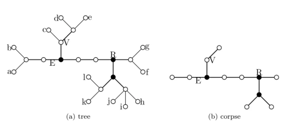
internal (i.e. non leaf) vertex v ∈ V (T ) corresponds to a partition Tv of A,
defined by the sets of leaves of the connected components of T \ v. Figure 1 shows an example of a partitioning tree. Similarly, any edge e ∈ E(T ) defines a
bi-partition Te of A. The ΦA width of (T, σ) is the maximum ΦA(T ) where T
is the partition defined by an internal vertex of T or an edge of T .
Definition 6. Let Φ be a partition function over A. The Φ-width of a set A ∈ A is the minimum ΦA width of its partitioning trees.
A branching node of tree T rooted in r ∈ V (T ) is either r or a vertex of T with at least two children. A tree T is q-branched if there exists a root r ∈ V (T ) such that any path from r to a leaf contains at most q ≥ 0 branching nodes. For instance, T is 0-branched if and only if T is a path.
Definition 7. The corpse cp(T ) of a tree T rooted in r ∈ V (T ) denotes the
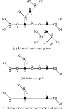
tree rooted in r obtained from T by removing all its leaves, but r if it is a leaf. In Figure 1, a 2-branched partitioning tree (T, R, σ) of the elements a, b,
. . . , k, l is represented. The vertex V ∈ V (T ) defines the partition TV with parts
{abf ghijkl, c, de}, R ∈ V (T ) defines the partition TR= {abcde, f g, hijkl}, and
the edge E ∈ E(T ) defines the bi-partition TE = {ab, cdef ghijkl}. The black
vertices are the branching nodes of cp(T ).
Definition 8. A partitioning tree (T, σ) is q-branched if the corpse cp(T ) of T
is q-branched.
For instance, a partitioning tree (T, σ) is 0-branched if and only if T is a
caterpillar1. The q-branched Φ-width of A is the minimum Φ
A width of its
q-branched partitioning trees.
R V a b c d e f g h i j k l E (a) tree R V E (b) corpse
Figure 1: A partitioning tree of {a, b, . . . , k, l} (a) and its corpse (b).
2.1
Graph Decompositions and Partitioning Trees
The notions from Section 2 have been given for general sets. In the following, we recall that partition functions and partitioning trees are generalization of several decompositions of graphs and their related parameters [AMNT09]. We assume that the reader is familiar the width measures of graphs such as tree width, branch width, cut width etc.
Throughout this section, E contains all possible edge-sets of every graph, i.e. for any graph G = (V, E) we have E ∈ E and V contains all possible vertex-set of every graph, i.e. for any graph G = (V, E) we have V ∈ V.
It is sometimes necessary, depending on the width measure, to restrict the shape of the partitioning tree, to add some constraint to the mapping of the leaves of the partitioning tree or to use a special partitioning function in order to express graph width measures in terms of partitioning functions and partitioning trees. In what follows, we show which restrictions are necessary to represent the special tree width, branch width, linear width, cut width and carving width in terms of partitioning functions and partitioning trees. We start by reproducing how the q-branched tree width of a graph can be represented by partitioning functions as shown in [AMNT09].
2.1.1 Partition function and q-branched tree width
For any graph G = (V, E), let ∆ be the function that assigns, to any partition
X = {E1, . . . , Er} of E, the set of the vertices that are incident to edges in Ei
and to edges in Ej, with i 6= j.
Definition 9. Let E ∈ E. The function δE is the partition function for E that
assigns |∆(X )| to any partition X of Part(E). Let δ be the partition function
over E that assigns δE to every E ∈ E .
Lemma 1. [AMNT09] For any graph G = (V, E), the tree width tw(G) of G is at most k ≥ 1 if, and only if, the δ width of E is at most k + 1.
Proof. In other words, we aim at proving that for any graph G = (V, E), the
tree width tw(G) of G is at most k if, and only if, there is a partitioning tree of E with δ width at most k + 1. Let (T, σ) be a partitioning tree of E with δ
width at most k + 1, then it is easy to check that (cp(T ), (Xt)t∈V (cp(T ))), with
(T, X ) be a tree decomposition of G with width at most k. Then, for any edge
{x, y} ∈ E, let us choose an arbitrary bag Xt that contains both x and y, add
a leaf f adjacent to t in T , and let σ(f ) = {x, y}. Finally, let S be the minimal subtree spanning all such leaves. The resulting tree (S, σ) is a partitioning tree of E with δ width at most k + 1.
A similar proof leads to:
Lemma 2. [AMNT09] For any graph G = (V, E), the path width pw(G) of G is at most k ≥ 1 if, and only if, there is a 0-branched partitioning tree (T, σ) of E with δ width at most k.
More generally:
Lemma 3. For any graph G = (V, E) and any q ≥ 0, the q-branched tree width
twq(G) of G is at most k ≥ 1 if, and only if, there is a q-branched partitioning
tree (T, σ) of E with δ width at most k.
The special tree width can be represented with the following restriction over the partitioning trees.
Special tree width: The special tree width of a graph can be expressed in
terms of the partition function δ, but with a restriction in the shape of the partitioning tree. For any graph G = (V, E), instead of searching
for the minimum δE width over all partitioning trees of E, we restrict the
partitioning trees to respect the following rule. Let (T, σ) be a partitioning
tree of E, for each vertex v in V , let T0 be the minimum subtree of (T, σ)
spanning all the leaves of (T, σ) such that their corresponding edge in E
has v as one extremity. We have that T0 is a caterpillar.
2.1.2 Other Widths and Partition Functions
The branch width and the linear width of a graph may be expressed in terms of the following partition function:
Definition 10. Let maxδE be the partition function for E ∈ E which assigns
maxi≤nδ(Ei, E \ Ei) to any partition (E1, . . . , En) of E. Let maxδ be the
partition function over E that assigns maxδE to any E ∈ E .
Branch width [BT97]: By definition, the branch width of G, denoted by
bw(G), is at most k ≥ 1, if and only if there is a partitioning tree (T, σ) of E with maxδ width at most k and such that the internal vertices of T have maximum degree at most three.
Linear width [BT04]: The linear width of G, denoted by lw(G) is defined as
the smallest integer k such that E can be arranged in a linear ordering (e1, . . . , em) such that for every i = 1, . . . , m−1 there are at most k vertices
both incident to an edge that belongs to {e1, . . . , ei} and to an edge in
{ei+1, . . . , em}. The linear width of G is at most k ≥ 2 if and only if there
is a partitioning tree (T, σ) of E with maxδ width at most k, such that the internal vertices of T have maximum degree at most three, and (T, σ) is 0-branched. This result easily follows from the trivial correspondence between such a partitioning tree of E and an ordering of E. Note that this does not hold for k = 1 (a 3 edges path is a counterexample).
The carving width of a graph may be expressed in terms of the following
partition function. For any partition X = {V1, . . . , Vr} of V ∈ V, let Edgeδ be
the function that assigns the cardinality of the set of the edges of the graph
G = (V, E) that are incident to vertices in Vi and Vj, with i 6= j.
Definition 11. Let maxEdgeδV be the partition function for V ∈ V that assigns maxi≤nEdgeδ(Vi, V \ Vi) to any partition (V1, . . . , Vn) of V . Let maxEdgeδ be
the partition function over V that assigns maxEdgeδV to any V ∈ V.
Carving width [ST94, TSB00]: The carving width of G, carw(G), by
defi-nition, is at most k ≥ 1 if and only if there is a partitioning tree of V with
maxEdgeδ width at most k, and such that the internal vertices of T have
maximum degree at most three.
The cut width of G, denoted by cw(G), is defined as the smallest integer k
such that V can be arranged in a linear ordering (v1, . . . , vn) such that for every
i = 1, . . . , n − 1 there are at most k edges both incident to a vertex that belongs
to {v1, . . . , vi} and to a vertex in {vi+1, . . . , vn}.
The partition function maxEdgeδ also may express the cut width of a graph
G = (V, E) when it is at least the maximum degree ∆ of G. Note that any
0-branched partitioning tree with maximum degree at most 3 is such that its
maxEdgeδ-width is at least ∆. On the other hand, any 0-branched partitioning
with maximum degree at most 3 of V can be seen as a linear ordering over the vertices of G, which implies that the maxEdgeδ-width of G is at least as big as cw(G). More precisely, the minimum maxEdgeδ width of the 0-branched partitioning trees of V with maximum degree at most 3 equals max{cw(G), ∆}. In general, to express the cut width of a graph, we need a more restrictive partition function.
Definition 12. Let 3-maxEdgeδV be the partition function for V ∈ V that
assigns the function max{Edgeδ(V1, V \ V1), Edgeδ(V2, V \ V2)} to any partition
(V1, V2, V3) of V , with |V3| = 1. Let 3-maxEdgeδ be the partition function over
V that assigns 3-maxEdgeδV to any V ∈ V.
Cut width [TSB00]: The cut width of G is at most k ≥ 1, if and only if
there is a partitioning tree (T, σ) of V with 3-maxEdgeδ width at most
k, and (T, σ) is 0-branched. This result easily follows from the trivial
correspondence between such a partitioning tree of V and an ordering of
V .
3
Main Results
In this section, we define properties of a partition function Φ that are sufficient for Φ to admit a linear-time (in the size of the input set) algorithm that decides whether the Φ-width of any set is at most k, k being a fixed integer.
More precisely, we start by giving a set of sufficient conditions for our theorem. Then, we show that all aforementioned widths respect these con-ditions. This implies that the algorithm in Section 6 can be used to compute all the aforementioned widths, thus this algorithm generalizes the FPT-algorithms of [BK96, BT97, TSB00, BT04].
3.1
Sufficient Conditions For a Linear Time Algorithm
First, some definitions are made in this section in order to state the main theo-rem.
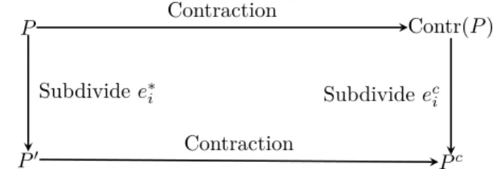
Since partitioning trees generalize the tree decomposition to any set (not only graphs), it is natural to extend the notion of nice tree decomposition [Bod96] to any set.
A nice decomposition (D, X ) of a finite set A is a O(|A|)-node rooted tree D,
together with a family X = (Xt)t∈V (D)of subsets of A such that, ∪t∈V (D)Xt=
A, for all a ∈ A the set {t | a ∈ Xt} induces a subtree of D, and for any
v ∈ V (D):
start node: v is a leaf, or
introduce node: v has a unique child u, Xu⊂ Xv and |Xv| = |Xu| + 1, or
forget node: v has a unique child u, Xv⊂ Xu and |Xu| = |Xv| + 1, or
join node: v has exactly two children u and w, and Xv= Xu= Xw.
The width of a decomposition (T, X ) is the maxt∈V (T )|Xt|. For any v ∈
V (D), let Dv denote the subtree of D rooted in v, and Av = ∪t∈V (Dv)Xt.
Let Φ be a partition function. A nice decomposition (D, X ) of a set A is
compatible with Φ if:
1. there exists a function FΦ that associates an integer FΦ(x, P, e) to any
integer x, partition P of some subset of A and element e of A, such that,
FΦis strictly increasing in its first coordinate, and, for any introduce node
v ∈ V (D) with child u, any partition P of Av,
ΦAv(P) = FΦ(ΦAu(P ∩ Au), P ∩ Xv, Av\ Au).
2. there exists a function HΦ that associates an integer HΦ(x, y, P) to any
pair of integers x, y, and partition P of some subset of A, such that, HΦ
is strictly increasing in its first and second coordinates, and, for any join
node v ∈ V (D) with children u and w, any partition P of Av,
ΦAv(P) = HΦ(ΦAu(P ∩ Au), ΦAw(P ∩ Aw), P ∩ Xv).
3. FΦand HΦhave time complexity that does not depend on the size of Av.
That is, they have constant time complexity with respect to the size of
Av.
4. If v ∈ V (D) is an introduction node with u as children, then for every
partition P of Av such that P ∩ Xv is a partition of Xv with only one
part, then ΦAv(P) = ΦAu(P ∩ Au).
If v ∈ V (D) is a join node with u and w as children, then for every
partition P of Av such that P ∩ Aw is a partition of Aw with only one
part we have that ΦAv(P) = ΦAu(P ∩ Au). Respectively, if P ∩ Au is a
Intuitively, the existence of FΦand HΦmeans that it is possible to quickly
compute the Φ-width of some partitions P without knowing explicitly P. By only knowing a restriction of P and the Φ-width of some restriction of P, these
restrictions being defined by the decomposition (D, X ). Moreover, the last
restriction over the function Φ means that changes on the width of a partitioning tree resulted from adding elements to the partitioning tree do not propagate
long. They are contained to vertices of the partitioning tree that partition Xv
into at least two parts.
3.2
Main Theorem
This is the main theorem of this paper:
Theorem 4. Let Φ be a monotone partition function that is closed under taking subsets. Let k, k0 ≥ 1 and q ≥ 0 be three fixed integers (q may be ∞). There
exists an algorithm that solves the following problem in time linear in the size of the input set:
input: a finite set A and a nice decomposition (D, X ), of width at most k0 for A, that is compatible with Φ,
output: decide if the q-branched Φ-width of A is at most k.
Corollary 1. Let Φ be a monotone partition function that is closed under taking subsets. Let k ≥ 1 and q ≥ 0 be 2 fixed integers (q may be ∞). Let A be a class of sets such that there exists a linear-time algorithm for computing a nice decomposition of width O(k) for any set A ∈ A, compatible with Φ, if it exists. There exists an algorithm that solves the following problem in time linear in the size of the input set:
input: a finite set A,
output: decide if the q-branched Φ-width of A is at most k.
The proof of Theorem 4 is quite technical and most of the remaining part of this paper is devoted to it. In order to explain such proof in a more didactic manner, we start with a simple algorithm to solve this problem, albeit not in linear time, and improve such algorithm in the following sections until we have a linear time algorithm.
3.3
Tractability of Width Parameters of Graphs
This section is devoted to present an application of Theorem 4 in terms of the width measures of graphs showed in Section 2.
Theorem 5. Let k and q be two fixed parameters. There exists an algorithm that solves the following problem in time linear in the size of the input graph.
input: A graph G with maximum degree bounded by a function of q and k, output: Decide if G has q-branched tree width, resp., branch width, linear
Proof. In Section 2, we explained that several width parameters of graphs
(q-branched tree width, resp., branch width, linear width, carving width, cut width or special tree width) can be defined in terms of partition functions. Therefore, the proof of Theorem 5 roughly consists in proving that the partition functions corresponding to these width parameters satisfy conditions of Theorem 4.
Bodlaender designs a linear-time algorithm that decides if the tree width of a
graph G is at most k0 (k0is a fixed parameter), and, if tw(G) ≤ k0returns a tree
decomposition of width at most k0[Bod96]. Moreover, a nice tree decomposition
of G can be computed in linear time from any tree decomposition of G, and without increasing its width [BK96]. Moreover, from Lemma 7, any nice tree decomposition of G can be turned into a nice decomposition of E(G) with width
at most dk0, where d is the maximum degree of G.
Note that from Lemmas 8, 9 and 10 we have that a nice decomposition is compatible with partitioning functions for q-branched tree width, branch width, linear width, carving width, cut width and special tree width. Therefore, in order to obtain a nice decomposition of E(G), we can use the algorithm in
[Bod96] and Lemma 7. Since, by hypothesis, the maximum degree of G is
bounded by a function of q and k, the width of the nice decomposition obtained is bounded by a fucntion of q and k. Therefore, the hypothesis of Theorem 4 is satisfied for all the aforementioned widths, which proves Theorem 5.
First, the following lemma is straightforward and its proof is thus omitted.
Lemma 6. The partition functions δ, maxδ, Edgeδ and maxEdgeδ are mono-tone and closed under taking subsets.
Next three lemmas show the compatibility of some nice decomposition with the partition functions δ, maxδ and maxEdgeδ.
Definition 13. [BK96] A nice tree decomposition of a graph G = (V, E) is a
tree decomposition of G that is a nice decomposition of V .
Lemma 7. Any nice tree decomposition (T, Y) of a graph G = (V, E) with width k can be turned into a nice decomposition (D, X ) of E. Moreover, if G has bounded maximum degree d, the width of (D, X ) is at most d · k.
Proof. For any v ∈ V (T ), let Tv denote the subtree of T rooted in v, and
Av = ∪t∈V (Tv)Yt, and let Ev be the set of edges belonging to the subgraph
induced by the vertices contained in Av that are incident to a vertex in Yv. Any
start node, resp., join node, Ytof (T, Y) corresponds to a start node, resp., join
node, Etof (D, X ). For any introduce node Ytof (T, Y), let x ∈ V be the vertex
such that Yt= Yt0∪{x}, where t0is the single child of t in T . Let e1, . . . , erbe the
edges that are incident to x and to some vertex in Yt0. Then, Ytis modified into
a path of introduce nodes E(G[Yt0]) ∪ {e1}, E(G[Yt0]) ∪ {e1, e2}, . . . , E(G[Yt0]) ∪
{e1, e2, . . . , er} in (D, X ). Finally, any forget node Yt of (T, Y) is modified
into a path of forget nodes E(G[Yt0]) \ {e1}, E(G[Yt0]) \ {e1, e2}, . . . , E(G[Yt0]) \
{e1, e2, . . . , er} in (D, X ), where t0 is the unique child of t in T , and e1, . . . , er
are the edges that are incident to x = Yt0 \ Yt and to no other vertex in Yt.
The obtained decomposition of E is a nice decomposition and its width (i.e. the maximum number of edges in each bag) is at most the width of the tree decomposition (T, Y) times the maximum degree of G.
Lemma 8. Let G be a graph with maximum degree deg. Given a nice tree decomposition (T, Y) of G with width at most k0 ≥ 1, a nice decomposition (D, X ) of E, compatible with the partition functions corresponding to tree width
(resp., path width and special tree width) and with maxt∈V (D)|Xt| ≤ k0· deg can
be computed in linear time.
Proof. Recall that the tree width, the path width and the special tree width of
a graph may be defined in terms of the partition function δ. First, let (D, X ) be
the nice decomposition of E, with width at most k0· deg, obtained from (T, Y)
as indicated in Lemma 7. We aim at proving that (D, X ) is compatible with δ.
Let Fδ be defined as follows.
Definition 14. Let x be an integer, P be a partition of a subset E0 of E and
an edge e ∈ E0. Let Fδ(x, P, e) = x + |{v ∈ e | v ∈ ∆(P) \ ∆(P ∩ (E0\ {e}))}|.
That is, Fδ adds to x the number of vertices incident to e that contribute
to the border of the partition P because they are incident to e. Fδ is obviously
strictly increasing in its first coordinate. Moreover, F can be computed in
constant time when |E0| is bounded by a constant.
For any v ∈ V (D), let Dv denote the subtree of D rooted in v, and Av =
∪t∈V (Dv)Xt.
Let v ∈ V (D) be an introduce node with child u, and let {e} = Xv\ Xu. Let
P be a partition of Av. We need to prove that δAv(P) = Fδ(δAu(P ∩ Au), P ∩
Xv, e). In other words, let us prove that δAv(P) = δAu(P ∩ Au) + |{v ∈ e | v ∈
∆(P ∩ Xv) \ ∆((P ∩ Xv) ∩ (Xv\ {e}))}|.
δAv(P) is the number of vertices in the subgraph induced by the set of edges
Av that are incident to edges in different parts of P. This set of vertices can
be divided into two disjoint sets: (1) the set S1 of vertices that are incident to
two edges f and h that are different from e and that belong to different parts
of P, and (2) the set S2of vertices x incident to e and such that all other edges
(different from e) incident to x belong to the same part of P that is not the
part of e. S1 is exactly the set of vertices belonging to ∆Au(P ∩ Au), therefore
|S1| = δAu(P ∩ Au).
By definition of (D, X ), because it has been built from a tree decomposition,
any edge of Au = Av\ {e} that has a common end with e belongs to Xv.
Therefore, any vertex in S2 belongs to ∆(P ∩ Xv). It is easy to conclude that
|S2| = |{v ∈ e | v ∈ ∆(P ∩ Xv) \ ∆(P ∩ Xv∩ (Xv\ {e}))}|.
Therefore, the function Fδ satisfies the desired properties.
Definition 15. Let x and y be two integers, and let P be a partition of a subset
E0 of E. Let Hδ(x, y, P) = x + y − δ(P).
Hδ is obviously strictly increasing in its first and second coordinates.
More-over, it can be computed in constant time when |E0| is bounded by a constant.
Let v ∈ V (D) be a join node with children u and w, and let P be a partition
of Av, we must prove that δAv(P) = Hδ(δAu(P ∩ Au), δAw(P ∩ Aw), P ∩ Xv).
That is, we prove that δAv(P) = δAu(P ∩ Au) + δAw(P ∩ Aw) − δXv(P ∩ Xv).
First, note that ∆Au(P ∩ Au) ∪ ∆Aw(P ∩ Aw) ⊆ ∆Av(P). Moreover, by
definition of the nice decomposition (D, X ), an edge of Au\ Xv and an edge
of Aw\ Xv cannot be incident. Indeed, Xv has been built by taking all edges
incident to a vertex in a bag Y of the tree decomposition (T, Y). By the connec-tivity property of a tree decomposition, if a vertex x would have been incident to
an edge in Au\ Awand to an edge in Aw\ Au, then x ∈ Y which would have
im-plied that both these edges belong to Xv = Au∩Aw, a contradiction. Therefore,
∆Av(P) ⊆ ∆Au(P ∩Au)∪∆Aw(P ∩Aw). To conclude showing that Hδis correct,
it is sufficient to observe that ∆Au(P ∩ Au) ∩ ∆Aw(P ∩ Aw) = ∆Xv(P ∩ Xv).
Now, we need to show that if v is an introduction node with u as children
then for all partitions P of Av such that P ∩ Xv is a partition of Xv with only
one part then ∆Av(P) = ∆Au(P ∩ Au).
Assume that v is an introduction node and that Av\ Au= {a}. Let P be a
partitioning of Av such that P ∩ Xv is a partition of Xv with only one part.
Since (D, X ) is a nice decomposition of E, we have that a is not adjacent to
any edge in Au\ Xv. Assume that ∆Au(P ∩ Au) < ∆Av(P). This means that
there is an extremity of a that is incident to an edge of Au\ Xv, a contradiction.
Therefore, ∆Au(P ∩ Au) = ∆Av(P).
Finally, we need to show that if v is a join node of (D, X ) with children u
and w, then for all partitions P of Avsuch that P ∩ Auis a partition of Au with
only one part then ∆Av(P) = ∆Aw(P ∩ Aw) or ∆Av(P) = ∆Au(P ∩ Au) in the
case that P ∩ Awis a partition of Aw with only one part.
W.l.o.g. assume that P ∩ Awis a partition of Awwith only one part. Since,
(D, X ) is a nice decomposition of E, we have that no edges in Au\ Aw share
extremities with edges in Aw\ Au. Moreover, (Au\ Aw) ∩ (Aw\ Au) = ∅ and
Au∩ Aw= Xv.
∆Av(P) is the number of vertices of G such that they are extremities for
edges in different parts of P. Since, P ∩ Aw is a partition with only one part
and the edges of Aw\ Au do not share any extremities with edges in Au\ Aw.
We have that ∆Av(P) is the number of vertices that are extremities of edges in
different parts of P ∩ Au. That is, ∆Av(P) = ∆Au(P ∩ Au).
The case where P ∩ Auis a partition of Auwith only one part is similar and
thus omitted.
It is easy to see that the partition function Edgeδ behaves as the δ function but the role of vertices and edges being reversed.
First note that any nice tree decomposition (T, Y) of G is a nice decomposi-tion of V . To prove that (T, Y) is compatible with the partidecomposi-tion funcdecomposi-tion Edgeδ, we follow the above proof of Lemma 8.
Definition 16. FEdgeδ and HEdgeδare defined as follows:
• Let x be an integer, P be a partition of a subset V0 of V and a vertex
v ∈ V0. Then,
FEdgeδ(x, P, v) = x+|{e ∈ E | v ∈ e and e ∈ Edgeδ(P)\Edgeδ(P∩(V0\{v}))}|.
• Let x and y be two integers, and let P be a partition of a subset V0 of V .
Then, HEdgeδ(x, y, P) = x + y − Edgeδ(P).
Therefore, the partition function Edgeδ is compatible with any nice tree decomposition. To prove the compatibility of the partition function maxEdgeδ with any nice tree decomposition, we use the following claim.
Let f be any partition function and let maxf be the partition function that
Claim 1. For any partition function f compatible with a nice decomposition of some set A, the partition function maxf is also compatible.
Remark 1. Claim 1 also serves to show that the partition functions for branch
width and linear width are also compatible to a nice decomposition of the edges of a graph.
Because f is compatible with any nice decomposition of A, there exist two
function Ff and Hf that satisfy the properties defining the notion of
compati-bility. We must have:
fAv(P) = Ff(fAu(P ∩ Au), P ∩ Xv, Av\ Au), and
fAv(P) = Hf(fAu(P ∩ Au), fAw(P ∩ Aw), P ∩ Xv).
The key point is that if P is a bipartition of some set A, then fA(P) =
maxfA(P). Therefore, when considering a bipartition, the functions Fmaxf and
Hmaxf can be defined similarly to Ff and Hf. The case that P is not a
biparti-tion is more technical, hence we postpone the proof of this claim until Secbiparti-tion 6 after showing how the algorithm works.
Hence with Claim 1 the partition functions corresponding to the branch width and linear width (carving width and cut width) are all compatible to nice decompositions of E (V ) of a graph G = (V, E). This gives us the following lemmas:
Lemma 9. Any nice decomposition (D, X ) of G is a nice decomposition of E compatible with the partition functions corresponding to branch width (resp., linear width).
Lemma 10. Any nice tree decomposition (T, Y) of G is a nice decomposition of V compatible with the partition functions corresponding to carving width (resp., cut width).
4
Describing Partitioning Trees in a Dynamic
Manner
In this section, we show the basic idea used to compute all the aforementioned widths.
4.1
Preliminary Definitions
Definition 17. Let (T, r, σ) be a rooted partitioning tree of a set A and A0⊆ A,
then the partitioning tree (T0, r0, σ0) of (T, r, σ) restricted to A0is the minimum
subtree of T0 spanning all the leaves corresponding to elements of A0. r0 is the
vertex of T0 that is closest to r in T and the function σ0 is the restriction of σ
to A0.
Let (D, X ) be a nice decomposition of a set A and Φ a partitioning function
of A that is compatible with (D, X ). Recall that for any v ∈ V (D), Dvdenotes
the subtree of D rooted in v, and Av= ∪t∈V (Dv)Xt. In what follows, a full set
all labeled q-branched partitioning trees of Φ-width at most k of Av. If r is the
root of (D, X ) then Ar= A, hence FSPTk,q(r) is not empty if and only if the
q-branched Φ-width of A is not bigger than k.
Definition 18. A labeled partitioning tree, ((T, r, σ), `) is a partitioning tree
(T, r, σ) along with a label `, a function from the edges or internal vertices of
T to integers, the label of a vertex (or edge) t of T is such that `(t) = Φ(At),
where Atis the partition of A defined by t.
The role of the label is to store the values of the partitioning function Φ for fast access and update during the execution of the algorithm.
4.2
Main Idea
Let k and q be fixed integers. The main idea behind the algorithm in section Section 6 is to use dynamic programming to compute a full set of partitioning trees for A by using a nice decomposition (D, X ) of A. In other words, to decide if the q-branched Φ-width of A is not bigger than k. We start by computing
a FSPTk,q(v) for all bags Xv where v is a leaf of D. Then, for each vertex
v ∈ V (D) such that for each child u of v we have already computed the set
FSPTk,q(u), we compute FSPTk,q(v). Once FSPTk,q(r), where r ∈ V (D) is
the root of D, is computed, then we can simply test if FSPTk,q(r) is empty to
decide whether the q-branched Φ-width of A is not bigger than k.
In this section we show how to compute FSPTk,q(v) for vertices of V (D),
for the moment, we do not focus on the complexity of this computation, rather we show the main idea behind each procedure introduced on Section 6. The
computation of FSPTk,q(v) depends on the type of the node v. In the following
subsections we show procedures for each kind of node in the nice decomposition (D, X ) (starting node, introduce node, forget node and join node).
We also state that it is possible that a full set of characteristics has infinite size, hence it is necessary to design a method to “compress” this set reducing its cardinality to something more manageable, i.e., a size given by a function bounded on k, the width of the nice decomposition and q. In Section 5 we show how this can be achieved.
Then, in Section 6, we show how to use this compression to design a linear time algorithm to decide if the Φ-width of a set A is not bigger than k, k being a fixed parameter.
4.3
Procedure Starting Node
If v is a starting node, i.e. a leaf of D. Then, procedure Starting Node consists
of enumerating all q-branched partitioning trees for Av with Φ-width at most
k.
That is, FSPTk,q(v) is the set of all possible labeled q-branched partitioning
trees for Av with Φ-width at most k.
Lemma 11. Let (D, X ) be a nice decomposition of a set A. The procedure Starting Node computes a full set of q-branched partitioning trees of Φ-width not bigger than k for a starting node v of D.
4.4
Procedure Introduce Node
Assume that v is an introduce node of D and that we aim at computing
FSPTk,q(v).
Let u be the only child of v in D and {a} = Xv\ Xu. Let FSPTk,q(u) be
the full set of labeled q-branched partitioning trees of Au with width at most
k. The set FSPTk,q(v) is obtained from FSPTk,q(u) by applying the following
procedure to every labeled partitioning tree (Tu, ru, σu) in FSPTk,q(u) and to
every possible execution of the step “update Tu into Tv”.
Procedure Introduce Node. Starting with FSPTk,q(v) =, for all possible
choices of step “update Tuinto Tv” and for all elements(Tu, ru, σu) ∈ FSPTk,q(u)
do the following:
update Tu into Tv: To insert a corresponding vertex to a in ((Tu, ru, σu), `u),
choose some internal vertex vatt of V (Tu), add a leaf vleaf adjacent to
vatt. Moreover, let enew = {vatt, vleaf}, we then proceed to subdivide
enew a finite number of times. Then, set σv(vleaf) = a. Let Pnew be the
path joining vleaf to vatt. If ru = vatt then rv is one of the vertices in
V (Pnew) \ {vleaf}, otherwise rv = ru. Note that, at this point, Tv is a
partitioning tree of Av.
update of labels of new vertex(s) and edge(s): First, let Pnewbe the path
joining vleaf to vatt. Then every internal vertex (or edge) p of Pnewreceives
label `v(p) = ΦAv({Au, {a}}).
update of labels of other vertex(s) and edge(s): For all e ∈ E(Tv)\E(Pnew),
let Tebe the partition of Xv defined by e. `v(e) ← FΦ(`u(e), Te, a). For
all t ∈ (V (Tv) \ V (Pnew)) ∪ {vatt}, let Ttbe the partition of Xv defined by
t, then `v(t) ← FΦ(`u(t), Tt, a).
update of FSPTk,q(v): If ((Tv, rv, σv), ellv) is q-branched, for every internal
vertex t ∈ V (Tv) we have `v(t) ≤ k and for every edge e ∈ E(Tv) we have
`v(e) ≤ k then FSPTk,q(v) ← FSPTk,q(v) ∪ {((Tv, rv, σv), `v)}, otherwise
FSPTk,q(v) remains unchanged.
Lemma 12. Let (D, X ) be a nice decomposition of a set A compatible with the monotone partition function Φ and let v be an introduce node of D with a child u. The procedure Introduce Node computes a full set of q-branched partitioning trees of Φ-width not bigger than k from the set FSPTk,q(u) for the node v.
Proof. Let FSPTk,q(v) be the set computed by the procedure Introduce Node,
we first show that any element ((Tv, rv, σv), `v) ∈ FSPTk,q(v) is a q-branched
partitioning tree with Φ-width not bigger than k for Av.
Let FSPTk,q(u) be a full set of q-branched partitioning trees of Φ-width not
bigger than k for the node u and let (Tu, ru, σu) be any element of FSPTk,q(u).
Assume that ((Tv, rv, σv), `v) is obtained through an execution of procedure
Introduce Node on (Tu, ru, σu).
From the step “update Tuinto Tv”, since (Tu, ru, σu) is a partitioning tree for
Auand Av\Au= {a}, taking (Tu, ru, σu) adding a leaf vleaf to an internal vertex
vattof Tuand mapping vleaf to a results in a partitioning tree for Av. Moreover,
the subdivision of {vatt, vleaf} does not change the fact that (Tv, rv, σv) is a
For any internal vertex (or edge) t of Tv let At be the partition of Av that
it defines. It remains to show that (Tv, rv, σv) is q-branched, has Φ-width not
bigger than k and that after the execution of the procedure Introduce Node all
labels are correct. In other words, for all internal vertices (or edges) t of Tv, we
prove that `v(t) = ΦAv(At).
In the step “update of FSPTk,q(v)”, ((Tv, rv, σv), `v) is only added to FSPTk,q(v)
if it is q-branched. Then, from the fact that there are only labeled
partition-ing trees in FSPTk,q(u), we have that `u(t) = ΦAu(At∩ Au) for any internal
vertex (or edge) t of Tu. Moreover, we have that Φ is compatible with the
nice decomposition (D, X ). Therefore, from the description of the Introduce
Node procedure for every internal node t (or any edge) of Tv that is not in
Pnew∪ {vatt}:
`v(t) = FΦ(`u(t), Tt, a) = FΦ(ΦAu(At∩ Au), At∩ Xv, a) = ΦAv(At).
Furthermore, all edges and internal vertices of Pnewreceive the label ΦAv({Au, {a}})
from step “update of new vertex(s) and edge(s)”, hence lv(t) = ΦAv({Au, {a}}),
where t is either an internal vertex of Pnew or an edge of Pnew. Lastly, again
from the fact that Φ is compatible with (D, X ) and from step “update of labels of other vertex(s) and edge(s):
`v(vatt) = FΦ(`u(vatt), Tvatt, a) = FΦ(ΦAu(Avatt∩Au), Avatt∩Xv, a) = ΦAv(Avatt).
Hence, at step “update of FSPTk,q(v)”, ((Tv, rv, σv), `v) is a labeled
par-titioning tree of Av. Therefore, the step “update of FSPTk,q(v)” guarantees
that ((Tv, rv, σv), `v) is only added to FSPTk,q(v) if it is a labeled q-branched
partitioning tree with Φ-width not bigger than k for Av. Thus, any element of
FSPTk,q(v) is a labeled q-branched partitioning tree with Φ-width not bigger
than k for Av.
We now show that any labeled q-branched partitioning tree with width not
bigger than k for Av is in FSPTk,q(v). Let ((Tv0, r0v, σ0v), `v) be any q-branched
partitioning tree with width not bigger than k for Av. Let (Tu, ru, σu) be
(Tv0, rv0, σv0) restricted to Au. The partitioning tree (Tu, ru, σu) is q-branched and
its Φ-width is not bigger than k, since we only remove branches when restricting
a partitioning tree and Φ is monotone. Thus, ((Tu, ru, σu), `u) ∈ FSPTk,q(u).
Let vleaf be the vertex of Tv0 that corresponds to a. Since Tu is a subtree
of Tv0, let vatt ∈ V (Tu) be the vertex that is closest to vleaf in Tv0 and Pnew be
the path in Tv0 joining vleaf to vatt. Since Au = Av\ {a}, all internal vertices
of Pnew have degree two in Tv0. Hence, Tv0 can be obtained from Tu in the step
“update Tu into Tv” by attaching the vertex vleaf to vatt and subdividing the
edge enew an amount of times equal to |V (Pnew\ {vleaf, vatt})|.
Therefore, let ((Tv, rv, σv), `v) be the labeled q-branched partitioning tree
obtained from ((Tu, ru, σu), `u) with the Introduce Node procedure by adding a
vertex vleaf mapping a to vatt and subdividing {vatt, vleaf} an amount of times
equal to |V (Pnew \ {vleaf, vatt})|. In other words, Tv and Tv0 are isomorphic.
Since the root of the tree does not change with the Introduce Node procedure,
r0v= rv = ru. Moreover, σv0 and σv are the same, i.e. σ0v= σv = σu∪ (vatt, a).
Therefore ((Tv0, r0v, σv0), `0v) = ((Tv, rv, σv), `v). Thus, for every q-branched
parti-tioning tree ((Tv0, rv0, σ0v), `v) with width not bigger than k for Av there is an
4.5
Procedure Forget Node
Let v be a forget node of D, u be its child and FSPTk,q(u) be a full set of labeled
q-branched partitioning trees of Au with width at most k. Then procedure
Forget Node consists of copying FSPTk,q(u). In other words, FSPTk,q(v) =
FSPTk,q(u).
Lemma 13. Let (D, X ) be a nice decomposition of a set A compatible with the monotone partition function Φ and let v be a forget node of D with a child u. The procedure Forget Node computes a full set of q-branched partitioning trees of Φ-width not bigger than k for a forget node v of D.
Since Av = Au we have that FSPTk,q(v) = FSPTk,q(u), therefore if v is a
forget node this procedure produces a full set of labeled q-branched partitioning
trees of Au with width at most k for the node v.
4.6
Procedure Join Node
Let v be a join node of D, u and w its children and FSPTk,q(u) a full set of
la-beled q-branched partitioning trees of Auwith width at most k and FSPTk,q(w)
a full set of labeled q-branched partitioning trees of Awwith width at most k.
Let ((Tu, ru, σu), `u) ∈ FSPTk,q(u) and ((Tw, rw, σw), `w) ∈ FSPTk,q(w).
The goal is to merge “compatible” partitioning trees. We recall that, by
def-inition of a join node of a nice decomposition, Xu = Xw = Xv. Hence, let
(Tr
u, rur, σur) be (Tu, ru, σu) restricted to Xv, i.e. the minimum subtree of Tu
span-ning all the leaves corresponding to elements of Xv(rruis the vertex of T
r u closest to ruin Tu), and (Twr, r r w, σ r
w) be (Tw, rw, σw) restricted to Xv. Then, we do the
following procedure for every pair of elements of ((Tu, ru, σu), `u) ∈ FSPTk,q(u)
and ((Tw, rw, σw), `w) ∈ FSPTk,q(w) such that Tur and Twr are isomorphic,
σur= σrwand for every possible execution of step “Identifying Tu and Tw”.
Identifying Tu and Tw: Tv is obtained by identifying all correspondent
ver-tices of Tur and Tvr. Then we remove from Tv the double edges resulting
from the identification process. The root of Tv is obtained arbitrarily
choosing an internal vertex of Tv. The mapping σv is obtained taking
both mappings σu and σw, i.e. the leaves that are in Tur and Twr keep
their correpondence to the elements of A. Since Xu = Xw = Xv, leaves
that correspond to elements of Xv have the same mapping in σu and σw.
Leaves that belong to Au\ Aw or Aw\ Au are only mapped by σu or σw
respectively. Note that, at this point, (Tv, rv, σv) is a partitioning tree of
Av.
Updating the labels: Let (Tr
v, rvr, σrv) be (Tv, rv, σv) restricted to Xv. Let tv
be a vertex of Tr
v and Ttv be the partition of Xv defined by tv. Let tuand
tw be the vertices of Tur and Twr, respectively, used to create tv. Then,
`v(tv) ← HΦ(`u(tu), `w(tw), Ttv). Let ev be an edge of T
r
v and Tev the
partition of Xv defined by ev. Let eu and ew be its correspondent edges
in Tr
u and Twr respectively. Then, `v(ev) ← HΦ(`u(eu), `w(ew), Tev). For
all other vertex (or edge) t of Tv: `v(t) ← `u(t) if t is a vertex (or edge)
Updating FSPTk,q(v): If ((Tv, rv, σv), `v) is q-branched, for every internal
ver-tex t ∈ V (Tv) we have `v(t) ≤ k and for every edge e ∈ E(Tv) we have
`v(e) ≤ k then FSPTk,q(v) ← FSPTk,q(v) ∪ {((Tv, rv, σv), `v)}, otherwise
FSPTk,q(v) remains unchanged.
Lemma 14. Let (D, X ) be a nice decomposition of a set A compatible with the monotone partition function Φ and let v be a join node of D with a child u and a child w. The procedure Join Node computes a full set of q-branched partitioning trees of Φ-width not bigger than k from the sets FSPTk,q(u) and FSPTk,q(w)
for the node v.
Proof. Using the same scheme for the correctness of procedure Introduce Node,
we first prove that all elements of FSPTk,q(v) described by the procedure Join
Node are in fact labeled q-branched partitioning trees with width not bigger
than k for Av.
Let ((Tu, ru, σu), `u) ∈ FSPTk,q(u) and ((Tw, rw, σw), `w) ∈ FSPTk,q(w), be
such that (Tu, ru, σu) restricted to Xu and (Tw, rw, σw) restricted to Xwsatisfy
the Join Node restrictions. In other words, let (Tr
u, rru, σur) and (Twr, rrw, σrw) be
(Tu, ru, σu) and (Tw, rw, σw) restricted to Xvrespectively. Then, Turand Twr are
isomorphic and σr
u= σrw.
The step “Identifying Tu and Tw” can be applied on ((Tu, ru, σu), `u) and
((Tw, rw, σw), `w). Since Av= Au∪ Aw, Xv= Xu= Xwand (Au\ Xu) ∩ (Aw\
Xw) = ∅, we have that (Tv, rv, σv) obtained through step “Identifying Tu and
Tw” is a partitioning tree of Av.
For any internal vertex (or edge) of Tv let Av be the partition of Av that
it defines. It remains to show that (Tv, rv, σv) is q-branched, has Φ-width not
bigger than k and that after the execution of the procedure Join Node all labels
are correct. In other words, for all internal vertices (or edges) t of Tv, we prove
that `v(t) = ΦAv(At).
In the step “update of FSPTk,q(v)”, ((Tv, rv, σv), `v) is only added to FSPTk,q(v)
if it is q-branched. Lastly, we have that Φ is compatible with the nice
decom-position (D, X ). Moreover, let At, for any internal vertex (or edge) t of Tv be
the partition of Av defined by t. Then, from the fact that ((Tu, ru, σu), `u) and
((Tw, rw, σw), `w) are labeled partitioning trees, `u(tu) = ΦAu(Atu∩ Au) for any
internal vertex (or edge) tuof Tuand `w(tw) = ΦAw(Atw∩ Aw) for any internal
vertex (or edge) tw of Tw. Therefore, from the description of the Join Node
procedure for every internal node (or any edge) of Tv:
`v(t) = HΦ(`u(t), `w(t), Tt) = HΦ(ΦAu(At∩Au), ΦAw(At∩Aw), At∩Xv) = ΦAv(At)
Hence, at step “update of FSPTk,q(v)”, ((Tv, rv, σv), `v) is a labeled
par-titioning tree of Av. Therefore, the step “update of FSPTk,q(v)” guarantees
that ((Tv, rv, σv), `v) is only added to FSPTk,q(v) if it is a labeled q-branched
partitioning tree with Φ-width not bigger than k for Av.
We now show that any labeled q-branched partitioning tree with width not
bigger than k for Av is in FSPTk,q(v). Let ((Tv0, r0v, σ0v), `v) be any q-branched
partitioning tree with width not bigger than k for Av.
Let (Tu, ru, σu) be (Tv0, r0v, σv0) restricted to Auand (Tw, rw, σw) be (Tv0, r0v, σv0)
restricted to Aw. The partitioning trees (Tu, ru, σu) and (Tw, rw, σw) are, by
def-inition of restriction, q-branched and their Φ-width is not bigger than k, thus
Let (Tr
u, rur, σur) and (Twr, rrw, σrw) be (Tu, ru, σu) and (Tw, rw, σw) restricted
to Xv respectively. Since Xu = Xw = Xv we have that (Tur, rru, σru) and
(Tr
w, rwr, σwr) are such that Tur and Twr are isomorphic and σur = σwr.
There-fore, the Join Node procedure is applied to (Tu, ru, σu) and (Tw, rw, σw).
Therefore, let ((Tv, rv, σv), `v) be the labeled q-branched partitioning tree
obtained from ((Tu, ru, σu), `u) and ((Tw, rw, σw), `w) with the Join Node
pro-cedure. Clearly, from the “Identifying Tu and Tv” step, Tv = Tv0 and σv = σv0.
Since the procedure Join Node chooses an arbitrary internal vertex as the root
of the partitioning tree, there is an execution of this step where rv is chosen as
the root of Tv. Therefore, ((Tv0, r0v, σv0), `0v) = ((Tv, rv, σv), `v).
4.7
Remarks on Width Measures
Given a graph G = (V, E) and a nice decomposition (D, X ) of E or V . Then,
with FSPTk,q(r) where r is the root of (D, X ), it is possible to answer if the (tree,
path, branch, linear, cut, carving) width of G is less or equal than k. For that,
we iterate among all ((T, r, σ), `) ∈ FSPTk,q(r) and search for one that obeys the
“structural” restrictions given by the desired width, for example, partitioning trees for the branch width are such that every internal vertex has degree three,
hence it is necessary to search FSPTk,q(r) for a labeled partitioning tree that
respects such restriction. In the case that there are no labeled partitioning trees with the “structural” restrictions given, then the desired width of G is bigger than k, otherwise we found a partitioning tree that proves that the desired width of G is not bigger than k.
The following sections of the paper address the fact that the number of
el-ements of FSPTk,q(v) is possibly infinite. In Section 5 we show how to store
FSPTk,q(v) in an efficient manner, by only storing “compressed” representatives
for each “class” of partitioning tree. Lastly, in Section 6, we show how to manip-ulate these compressed representatives in order to design an algorithm for this problem. This manipulation is a direct extension of the procedures Start Node, Introduce Node, Join Node and Forget Node when applied to “compressed”
representatives of FSPTk,q(v).
5
Good Representatives of Partitioning Trees
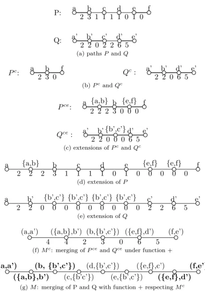
In this section we outline the ideas used in order to improve the space necessary to store the q-branched partitioning trees of a node in the nice decomposition of A. In other words, in this section, we reuse a method for “compressing” path decompositions and tree decomposition in [BK96] this time applied to q-branched partitioning trees and partitioning functions. A “compression” of the
set FSPTk,q(v) for a node v of the nice decomposition of A is such that the
size of this compression is bounded by q, the Φ-width and the width of the nice decomposition of A. Hence, it does not depend on the size of A. Intuitively, this is achieved by keeping only “good” representatives, a.k.a. characteristics, for each q-branched partitioning tree with Φ-width at most k of A.