Comparison of Charge-Exchange Recombination Spectroscopy Measurements of the Pedestal Region of Alcator C-Mod with Neoclassical Flow Predictions

January 2010

Plasma Science and Fusion Center Massachusetts Institute of Technology

Cambridge MA 02139 USA

This work was supported by the U.S. Department of Energy, Grant No. DE-FC02-

99ER54512. Reproduction, translation, publication, use and disposal, in whole or in part, by or for the United States government is permitted.

PSFC/RR-10-01 DOE/ET-54512-370

Comparison of Charge-Exchange

Recombination Spectroscopy Measurements

of the Pedestal Region of Alcator C-Mod

with Neoclassical Flow Predictions.

Comparison of Charge-Exchange Recombination

Spectroscopy Measurements of the Pedestal

Region of Alcator C-Mod with Neoclassical Flow

Predictions

by

Kenneth David Marr

Submitted to the Department of Physics

in partial fulfillment of the requirements for the degree of

Doctorate of Philosophy in Plasma Physics

at the

MASSACHUSETTS INSTITUTE OF TECHNOLOGY

January 2010

c

Massachusetts Institute of Technology 2010. All rights reserved.

Author . . . .

Department of Physics

January 7, 2010

Certified by . . . .

Dr. Bruce Lipschultz

Senior Scientist, Plasma Science and Fusion Center

Thesis Supervisor

Certified by . . . .

Dr. Earl Marmar

Senior Scientist, Department of Physics

Thesis Supervisor

Accepted by . . . .

Comparison of Charge-Exchange Recombination

Spectroscopy Measurements of the Pedestal Region of

Alcator C-Mod with Neoclassical Flow Predictions

by

Kenneth David Marr

Submitted to the Department of Physics on January 7, 2010, in partial fulfillment of the

requirements for the degree of Doctorate of Philosophy in Plasma Physics

Abstract

The study and prediction of velocities in the pedestal region of Alcator C-Mod are important aspects of understanding plasma confinement and transport. In this study, we examine the simplified neoclassical predictions for impurity flows using equations developed for plasmas with background ions in the Pfirsch-Schl¨uter (PS, high col-lisionality) and banana (low colcol-lisionality) regimes. Measured B5+ _{flow profiles are}

derived from the charge-exchange spectroscopy diagnostic on Alcator C-Mod and are compared with calculated profiles for the region just inside the last closed flux surface. For the steep gradient region, reasonable agreement is found between the predictions from the PS regime formalism and the measured poloidal velocities regardless of the collisionality of the plasma. The agreement between the neoclassical predictions us-ing the banana regime formalism and measured velocities is poorer. Additionally, comparisons of measured velocities from the low- and high-field sides of the plasma lead us to infer the strong possiblity of a poloidal asymmetry in the impurity density. This asymmetry can be a factor of 2–3 for the region of the steepest gradients, with the density at the high-field side being larger.

Thesis Supervisor: Dr. Bruce Lipschultz

Title: Senior Scientist, Plasma Science and Fusion Center Thesis Supervisor: Dr. Earl Marmar

Acknowledgments

First and foremost, I would like to thank Dr. Bruce Lipschultz for many years of advice, concern, support, and friendship. I doubt I would have made it through this process without his constant encouragement and prodding. It was not always easy for either of us, but together we have made it to a successful end. I cannot express how much I appreciate how flexible he has been with all the weekend meetings, eleventh hour turn-ins, and other situations too numerous to mention. Lastly, I’d like to thank him for all the advice on scientific writing that has gone into this thesis. He has been a good friend and a great advisor.

I would like to give my appreciation to my thesis readers and committee who have guided me through this process. Prof. Miklos Porkolab has provided years of advice as my academic advisor as well as acting as my thesis reader. Dr. Earl Marmar has acted as my co-supervisor and his comments on my thesis were invaluable. Prof. John Belcher worked closely with me when I was a teaching assistant for 8.02TEAL, which I enjoyed thoroughly. I thank him for being part of my committee as well.

I am eternally grateful to Prof. Peter Catto and Dr. Andrei Simakov, who not only provided much of the work simplifying the theoretical models used in this thesis, but also took the time to explain the various concepts to me when I was struggling with them. Without their support I would not have been able to properly address all the concepts presented here. Additionally, Dr. Grigory Kagan provided all the hard work behind the drift kinetic effect discussed in Chapter 5.

I would like to thank Dr. Jim Terry who worked with me during my first years here and has constantly and cheerfully answered my questions over the remaining years. Similarly, I would like to thank Dr. Brian LaBombard for always being available whenever I had a question about anything. I would also like to thank the other scientists, both from C-Mod and collaborators, who have also supported my progress throughout the years. These include: Dr. P. Bonoli, Dr. C. Fiore, Dr. R. Granetz, Dr. M. Greenwald, Dr. A. Hubbard, Dr. J. Hughes, Prof. I. Hutchinson, Dr. J. Irby,

Dr. Y. Lin, Dr. D. Mikkelsen, Prof. R. Parker, Dr. J. Rice, Dr. W. Rowan, Dr. S. Scott, Prof. D. Whyte, Dr. S. Wolfe, Dr. S. Wukitch, and Dr. S. Zweben.

I would like to thank all the graduate students who have worked alongside me and helped me in numerous ways. Rachael McDermott deserves very special mention and an amazing amount of gratitude for all her work with CXRS diagnostic. Similarly, R. Michael Churchill has stepped up and taken over operations of the CXRS diagnostic so that I could focus more on the analysis of this data. I also have to say that Aaron Bader rocks! He has been a constant source of advice, support, superb friendship, and correct grammar. He uncomplainingly read anything I asked him to correct and did not spare the red pen as he did. Similarly, my officemates Kirill Zhurovich and Greg Wallace were always supportive, cheerful, and helpful. I’d also like to thank Brock B¨ose, Alex Graf, Jinseok Ko, Orso Meneghini, Yuri Podpaly, Andr´ea Schmidt (and husband Sal), Shunichi Shiraiwa, Noah Smick, Kelly Smith, Vincent Tang, and Balint Veto for years of friendship both inside and outside the lab. Over the years several other graduate students and postdoctoral researchers have come and gone from my life and I would like to mention them now, although I cannot express all they have done for me: Sarah Angelini, Harold Barnard, Igor Bespamyatnov, Chris Boswell, Alex Boxer, Dan Brunner, Antoine Cerfon, Istvan Cziegler, Arturo Dominguez, James Dor-ris, Eric Edlund, Jennifer Ellsworth, Marco Ferrara, Will Fox, Sanjay Gangadhara, Tim Graves, Soren Harrison, Zachary Hartwig, Nathan Howard, Alex Ince-Cushman, Thomas Jennings, Noam Katz, Shinya Kurebayashi, Matt Landreman, Liang Lin, John Liptac, Larry Lyons, Scott Mahar, Dan Miller, Bob Mumgaard, John Nazemi, Roman Ochoukov, Felix Parra-Diaz, Matt Reinke, Jason Sears, and Howard Yuh.

The administrative staff at the PSFC has been more than supportive during my education and research. In fact, some have also become my friends and I would like to share my appreciation of them. Jessica Coco, Valerie Censabella, and Megan Tabak have all been exceptional in their service and friendship. Special thanks to Valerie for setting up the Alcator softball team every year and to Jessica for helping

out with my posters as well as preparing the food for my defense. Several others also deserve thanks and mention: Carol Arlington, Tim Davis, Matt Fulton, Tom Hrycaj, Lee Keating, Nancy Masley, Paul Rivenberg, Jason Thomas, and Dragana Zubcevic. I’d also like to thank the custodial staff for all their hard work, which is never appreciated enough. Finally, I’d like to thank the Physics Department staff, especially Brian Canavan, for all their help.

My research would not have been possible without the tireless work and support of the engineers and technicians that work at the PSFC. Special thanks go to Ed Fitzgerald, Jim Irby, and Henry Bergler for all their help and support. Bob Childs, Ron Rosati, Tom Toland, and Patrick Scully in the vacuum shop were always willing to lend me a helping hand or a tool, as long as it came back. Dave Bellofatto, William Burke, Wade Cook, Maria Silveira and Bruce Wood in the electronic shop were prompt and skilled in their work and always would share a smile in the hallway. I owe special thanks to Josh Stillerman who has repeatedly helped me troubleshoot several different problems throughout the years. Other staff that have earned my gratitude are: Sue Agabian, Dexter Beals, Bill Byford, Charlie Cauley, Gary Dekow, Thomas Fredian, Mark Iverson, Dave Johnson, Atma Kanojia (also for his friendship), Felix Kreisel, Mark London, Rick Murray, Don Nelson, Bill Parkin, Andy Pfeiffer, Edgar Rollins, Brandon Savage, Frank Shefton, Bob Sylvia, and Rui Viera.

I have to also thank all my friends from Torrance High, Principia College, and those I have made in the Boston area, who have supported me and cheered me on during the hardest times. Specifically, Toby Dusette, David Korka, Matt Pressler, and Rommel Tawatao were always there when I needed them and I couldn’t ask for better friends. All my roommates deserve special mention for putting up with me and the strange hours I’ve kept: Liz Heining, Annabel Hossell, Morgan James, William Lopes, Jon Noltie, Rich Redemske, and Mat Willmott. Also, I’d like to give a shout out to all the Puffywumps and the folks in <Casualty>. Additionally, I’d like to thank all my friends in the MIT Concert Band and specifically the band conductors,

Stephen Babineau and Thomas Reynolds. Lastly, I’d like to thank Monica Oyama, my cat Smokey, and my especially family, David, Marilyn, Robert, and Rebecca, all of whom have kept me sane and always knew how to make me smile.

Thanks again to everybody. This thesis would not have been possible without you.

Contents

1 Introduction 21

1.1 Alcator C-Mod . . . 22

1.1.1 Plasma operations . . . 25

1.1.2 Pedestal Region . . . 27

1.1.3 Relevant diagnostics and systems . . . 29

1.2 Thesis goals and outline . . . 33

2 The Edge CXRS Diagnostic on Alcator C-Mod 35 2.1 In-vessel components . . . 37

2.1.1 Low-field side imaging systems . . . 38

2.1.2 High-field side imaging system . . . 41

2.2 External components . . . 44

2.2.1 Spectrometers . . . 45

2.2.2 Cameras . . . 45

2.2.3 Choppers and chopper control . . . 48

2.2.4 CPLD system and the A/D Digitizer . . . 48

2.3 Spectral Analysis . . . 49

2.3.1 Calibrations . . . 50

2.3.2 Background subtraction . . . 53

2.3.3 Zeeman splitting . . . 56

3 Background 63

3.1 Transport and collisionality regimes . . . 63

3.1.1 Classical transport . . . 63

3.1.2 Neoclassical transport . . . 65

3.1.3 Collisionality Regimes . . . 67

3.2 Flow on a flux surface . . . 70

3.3 Profile Alignment . . . 71

3.3.1 Thermal equilibration . . . 71

3.3.2 Alignment of HFS data . . . 73

3.3.3 Te and Tz profiles . . . 75

4 Measurements and trends from the high-field side CXRS diagnostic 79 4.1 Low confinement . . . 80

4.1.1 L-mode operation . . . 80

4.1.2 Trends in the CXRS data during L-mode operation . . . 83

4.1.3 Density dependence of the parallel velocity . . . 86

4.2 High confinement . . . 87

4.2.1 EDA H-mode operation . . . 87

4.2.2 ELM-free H-mode operation . . . 90

4.2.3 Increased velocity shear in reversed field operation . . . 91

5 Comparison of measured and neoclassical LFS poloidal velocities 95 5.1 Predicting the low-field side poloidal velocity . . . 97

5.2 Comparison of measured and predicted velocities at the LFS . . . 98

5.2.1 Poloidal rotation in the steep gradient region . . . 98

5.2.2 Sensitivity to the position of the TS profiles . . . 103

5.2.3 Comparison to NEO . . . 105

5.2.4 Rotation at the top of the pedestal . . . 107

5.3 Discussion . . . 111

6 Measured high-field side parallel velocity and the poloidal asymme-try in the impurity density 113 6.1 Comparison of the measured and predicted velocities at the HFS . . . 114

6.2 Poloidal asymmetry in nz . . . 117

6.2.1 Modification of the neoclassical equations . . . 120

6.2.2 Inferred asymmetry . . . 123

6.2.3 Uncertainty . . . 126

6.2.4 Correlation with the poloidal velocity . . . 126

6.2.5 Sensitivity to the poloidal velocity . . . 128

6.3 Neoclassical prediction of asymmetry . . . 129

6.4 Summary and discussion . . . 130

7 Summary 133 A Appendix: Diagnostic Specifications 139 A.1 Overview . . . 139

A.2 The MPB and A/D digitizer . . . 141

List of Figures

1-1 Cut-away view of Alcator C-Mod . . . 23

1-2 Cross section of C-Mod . . . 24

1-3 Sketch of LSN, DN, and USN magnetic topologies . . . 26

1-4 Time traces of plasma parameters for an EDA H-mode . . . 27

1-5 Time traces of plasma parameters for ELM-free H-mode . . . 28

1-6 Representative Te and ne profiles in the pedestal region . . . 29

1-7 Top view of C-Mod . . . 30

2-1 In-vessel photo of F-port showing LFS periscopes . . . 38

2-2 Lines-of-sight for both poloidal and toroidal viewing LFS periscopes . 41 2-3 Location of the foci of the LFS periscopes in the DNB path . . . 42

2-4 Lines-of-sight for the HFS parallel viewing periscope and GPI puff locations . . . 44

2-5 Schematic of the spectrometer and camera system . . . 46

2-6 Photo of the spectrometer and camera, including the mounting and focusing platforms . . . 47

2-7 Example CXRS spectra from both the HFS and LFS . . . 50

2-8 Example fit to the neon spectrum for wavelength calibration . . . 51

2-9 Comparison of the total and background spectra . . . 54

2-10 The ratio of the integrated brightness of the B V lines from the signal and background views during a LSN shot . . . 56

2-11 The ratio of the integrated brightness of the B V lines from the signal

and background views during an USN shot . . . 57

2-12 The Zeeman split fine structure for the n = 7 → 6 transition . . . 58

2-13 The Blom and Jup´en parametrization of the Zeeman effect . . . 59

2-14 Fit to the active signal after the background has been subtracted . . 61

3-1 The classical and neoclassical diffusion coefficients by collisionality . . 66

3-2 The Tz,HFS, Tz,LFS and Te profiles before and after shifting . . . 72

3-3 The equilibration times between the majority ion, impurities, and elec-trons in the pedestal region . . . 74

3-4 A graphical representation of the variables used to fit a hyperbolic tangent to the pedestal data . . . 75

3-5 Comparison of scale lengths in the pedestal region . . . 77

3-6 Comparison of Tz to Te . . . 77

4-1 Four magnetic field configurations . . . 81

4-2 Relevant plasma parameters from an L-mode LSN discharge . . . 82

4-3 HFS parallel velocity profiles from an L-Mode LSN discharge . . . 83

4-4 HFS impurity temperature profiles from an L-mode LSN discharge . . 84

4-5 The HFS parallel velocity profiles determined through passive analysis 85 4-6 The HFS parallel velocity profiles determined through active analysis 86 4-7 Relevant plasma parameters from an EDA H-mode LSN discharge . . 88

4-8 HFS parallel velocity profiles from an EDA H-mode LSN discharge . 89 4-9 HFS impurity temperature profiles from an EDA H-mode LSN discharge 89 4-10 Relevant plasma parameters from an ELM-free H-mode, LSN, reversed-field discharge . . . 90

4-11 HFS parallel velocity profiles from several times during a ELM-free H-mode, LSN, reversed field discharge . . . 92

4-12 HFS impurity temperature profiles from several times during a ELM-free H-mode, LSN, reversed field discharge . . . 92 4-13 Time traces of the HFS impurity temperature and the stored energy . 93 4-14 Representative velocity profiles showing the increased shear in reversed

field operation . . . 94

5-1 Representative radial profiles of the measured and predicted poloidal velocities . . . 99 5-2 Comparison of the widths of the peaks in the Vz,θ and Vz,θPS profiles . . 101

5-3 Comparison of the positions of the peaks in the Vz,θ and Vz,θPS profiles. 102

5-4 Comparison of the peak heights from the Vz,θ, Vz,θPS, and Vz,θb profiles . 103

5-5 Representation of the sensitivity of the predicted profiles to the relative positions of the ne and Tz profiles . . . 104

5-6 A single case comparison of the results from NEO with the measured poloidal velocity . . . 106 5-7 Comparison of predicted and measured velocities for radii well inside

the steep gradient region . . . 107 5-8 The shaping function, J, for the banana regime formalism . . . 109 5-9 Effect of the drift kinetic effect on the calculated Vb

z,θ profile . . . 110

6-1 Radial profiles of all the velocities measured by the CXRS diagnostic 115 6-2 Radial profiles of uz(ψ) and ωz(ψ) . . . 116

6-3 Profiles of the predicted and measured HFS parallel velocity . . . 116 6-4 Scatter plot of the measured and predicted parallel HFS velocities . . 118 6-5 The inferred HFS impurity density mapped to the LFS and the

mea-sured LFS impurity density . . . 122 6-6 The inferred asymmetry for the entire dataset . . . 124 6-7 The dependence of the asymmetry on the poloidal velocity . . . 127 6-8 The effect on the inferred asymmetry of a small increase to Vz,θ . . . 128

6-9 The predicted asymmetry for the current dataset . . . 131 A-1 Schematic of the CXRS system before the addition of the CPLD board 141 A-2 Time traces of the driving clock, chopper, and digitization signals . . 143 A-3 Effect on the chopper phases of the adjustment by the CPLD board . 145 A-4 Photo of the CPLD system . . . 145

List of Tables

A.1 CPLD 2-Pin LEMO external connections . . . 146 A.2 CPLD ribbon cable signals to the A/D digitizer . . . 147 A.3 Necessary CPLD jumpers . . . 147

Commonly used acronyms and

symbols

CXRS Charge exchange recombination spectroscopy

DNB Diagnostic neutral beam

ICRF Ion cyclotron range of frequency NINJA Neutral injection apparatus

TS Thomson Scattering diagnostic

LCFS Last closed flux surface

SOL Scrape-off layer

LFS, L Low-field side

HFS, H High-field side

LSN Lower single null

USN Upper single null

FWHM Full width at half maximum

A Asymmetry

V Velocity

θ Poloidal or poloidal coordinate

φ Toroidal or toroidal coordinate

k Parallel

⊥ Perpendicular

b banana T Temperature n Density p Pressure i Majority ions z Impurity ions

e Electrons or charge of an electron

Z Charge state

n Energy level of an electron in an atom

R Major radius

ft Fraction of particles that are trapped

fc Fraction of particles that are circulating

ψ Flux coordinate

u(ψ), k(ψ), ω(ψ) Values that are constant on a flux surface

ρ Larmor radius

L Scale length

h i Flux surface average

r/a Normalized distance from the center of the plasma as measured at the LFS midplane

ρpeak Distance from the peak in the measured

poloidal velocity profile

Er Radial electric field

J(u/vth) Shaping term from the drift kinetic effect

u Measure of the radial electric field

vth Thermal velocity

M Mach number

U Uncertainty

Chapter 1

Introduction

The Alcator project was started at the Plasma Science and Fusion Center of the Massachusetts Institute of Technology in 1972 with the initial operation of Alcator A, a compact, wall-limited, high-field, high-density, fusion device [1]. The name is derived from Italian, ALto CAmpo TORus, meaning “high field torus.” The current incarnation of the project is Alcator C-Mod, a significantly larger and diverted fusion device, which has been in operation since 1993 with the goal of studying plasma physics and fusion technology [2]. Alcator has been funded by the United States Department of Energy since the project’s inception and C-Mod is one of three large-scale tokamaks currently in operation in the USA [2, 3, 4].

Alcator C-Mod is part of the larger fusion community which spans several con-tinents and is working towards a sustainable source of energy to supply humanity’s growing energy needs. The Alcator project is dedicated to understanding plasma physics in order to provide future fusion devices with the knowledge of how to create hotter, more dense, and better confined plasmas. The recent focus of the magnetically-confined fusion community is the ITER project currently being con-structed in Cadarache, France and expected to start operation in 2018 [5]. ITER is a long-pulse fusion device, larger than any built yet, and is designed to produce a net gain in energy, a state where the self-heating due to fusion produced alpha particles

is the dominant heat source for the plasma [6]. Therefore, it is of utmost importance to understand all aspects of plasma dynamics, and how they scale with size, as we prepare for ITER and future fusion devices.

One particular aspect of plasma physics that has received significant attention in the last few decades is particle velocity and its role in setting the energy transport. Near the plasma edge, turbulent transport causes particle loss, reducing confinement of energy and particles [7]. Increased velocity shear in this region is thought to break up turbulent structures and increase energy confinement times [8, 9, 10]. However, the mechanisms that drive particle flows are still poorly understood and models that seek to explain them are not fully tested. The high densities of Alcator C-Mod provide a unique opportunity to study both measured and predicted velocities in a strongly collisional plasma.

1.1

Alcator C-Mod

Alcator C-Mod is a toroidal fusion device with a major radius of 66.5 cm and a minor radius of ∼22 cm [11]. Figure 1-1 shows a cut-away view of the tokamak and surrounding components. The surfaces facing and interacting with the plasma are primarily molybdenum tiles which are designed to handle the high heat loads typical during normal operation. To improve performance, those “first-wall” surfaces are often coated with a thin layer of boron, which can quickly wear away during operation [12]. Boron is preferable to molybdenum as a first surface because boron has fewer bound electrons at the temperatures found in the plasma and thus radiates less energy. As seen in Figure 1-2, a stainless steel cylinder and two 66 cm thick stainless steel disks hold the machine together during the extreme forces generated by the magnetic fields [11]. These structural components are held together by ninety-six INCONEL bolts, which compress the plates together at all times. Liquid nitrogenR is pumped into the cryostat to cool the copper magnets which create the magnetic

Figure 1-1: Cut-away view of Alcator C-Mod.

fields to about −170◦_{C. 1.5 m thick concrete blocks, which absorb neutrons produced}

during fusion, surround the cryostat and protect nearby equipment.

C-Mod discharges typically last for ∼2 s and 30–35 plasma discharges are created per day. Most experiments use deuterium (D), an isotope of hydrogen (H), as the primary ion species, though plasmas may be made from other gases such as hydrogen or isotopes of helium (He3 and He4). Ramping current through a solenoid located in the central column of the tokamak inductively drives an ohmic (OH) current toroidally through the gas, inducing ionization [11]. Typical operation can generate currents between 0.4–2.0 MA. The plasma is confined via a strong toroidal magnetic field (TF) generated from a single 120-turn, toroidal solenoid, copper electromagnet. This magnet is capable of producing fields up to 8 T in the center of the plasma. The toroidal magnetic field has a 1/R dependence, being strongest next to the central

Figure 1-2: A cross section of C-Mod showing the last closed flux surface in lower single null configuration. Also shown is the path of the diagnostic neutral beam (DNB).

column and becoming weaker with increasing major radius. The toroidal current flowing in the plasma creates a weak, poloidal magnetic field, giving the total field a helical shape. Additionally, toroidally wound magnets are used to control the elongation and the triangularity of the plasma. Electron densities in the core of the plasma can range from 1019_–1021 _m−3_{. Core electron temperatures}1 _{are typically}

between 1.5–6.0 keV.

1

Large temperatures, such as those found in C-Mod, are typically expressed in electron-Volts. 1 eV = 11,604 K.

1.1.1

Plasma operations

In the plasma, magnetic field lines trace out nested flux surfaces as they loop toroidally and poloidally around the tokamak. “Closed” flux surfaces are those that do not in-tersect a material surface. The last closed flux surface (LCFS) separates the closed surfaces from the scrape-off layer (SOL) where field lines terminate on machine sur-faces. In a diverted plasma, such as those usually created by C-Mod, particles and energy in the SOL will flow along field lines toward the divertors at the top and bot-tom of the vessel [13]. Due to topological considerations in a diverted configuration, there are two nulls, or x-points, where the poloidal magnetic field must disappear. The flux surface containing the null point closest to the plasma axis is called the primary “separatrix,” which is also the LCFS for diverted plasmas. If both x-points are located inside the vessel structure, the plasma is considered to be “wall limited,” similar to early tokamak operations. Standard C-Mod operation has a single null near the bottom of the machine. Figure 1-2 shows the LCFS in this lower single null (LSN) configuration. Often, experiments will call for discharges with upper single null (USN) or even double null (DN, both upper and lower) topologies. Representations of these magnetic topologies are shown in Figure 1-3.

Several operating regimes are available to C-Mod [14]. The simplest plasmas are Ohmically driven with low confinement, or L-mode plasmas. High confinement op-eration, or H-mode, is characterized by an edge transport barrier to particles and energy [15]. It is possible to cause a low-to-high (L-H) transition [15] in an Ohmic plasma, for example by lowering the magnetic field during the discharge, but these Ohmic H-modes are often difficult to achieve and maintain. A more reliable method of obtaining H-mode operation is to heat the plasma through the injection of auxillary power, such as ion-cyclotron range of frequency (ICRF, see section 1.1.3) wave ab-sorption [16]. Ohmic and RF-heated H-mode plasmas routinely develop edge modes, which generally degrade particle or energy confinement through loss of plasma [17]. The most common of these modes for C-Mod is the quasi-coherent (QC) mode, which

Lower

Single

Null

Upper

Single

Null

Double

Null

Figure 1-3: Sketches of the LCFS and a single SOL field line in LSN, DN, and USN magnetic topologies.

continually expels small amounts of the plasma into the SOL, and is the defining char-acteristic of the enhanced Dα (EDA) H-mode [18].2 Although the QC mode reduces

particle confinement, it also allows the H-mode regime to persist in a stationary state by removing impurities from the core. Figure 1-4 shows time traces of the various plasma parameters, such as the density and magnetic oscillations, during an EDA H-mode discharge. Another edge mode that may occur during H-mode operation is the discrete (in time) Edge Localized Mode (ELM), wherein plasma is ejected into the SOL causing a brief spike in the Dα emission [20]. These events are uncommon

in standard C-Mod operation, but it is possible to recreate ELMy plasmas for com-parison to other tokamaks [21]. It is also possible for C-Mod plasmas to enter an ELM-free H-mode, where impurities, with no loss mechanism from either ELMs or the QC mode, accumulate in the core [14]. The build up of pressure and radiation eventually collapses the edge transport barrier and the plasma returns to L-mode confinement. Figure 1-5 shows relevant plasma parameters for an ELM-free H-mode discharge.

2

The steady ejection of plasma causes an elevated emission of Dα light as this plasma cools on

2 Time (s) 0.6 0.8 1.0 1.2 1.4 1.6 0.4 4 150 50 0.6 1.0 2 4 1 0.5 1.5 2 4 0 0.2 0 3 (a) (b) (c) (e) (f) (d) 0 (g) Temperature (keV) Density (1020m-3) P-Rad (MW) D-alpha H98 Magnetic Fluctuations (kHz) RF Power (MW)

Figure 1-4: Time traces for the a) Dα brightness b) radiated power c) core electron

density d) core electron temperature e) H89 f) magnetic fluctuations and g) injected

ICRF power during an EDA H-mode discharge. [19]

1.1.2

Pedestal Region

The pedestal region is roughly defined as the plasma of several centimeters radial width inside the LCFS where the density and temperature of the plasma increase sharply (moving into the plasma) during H-mode operation [22]. Figure 1-6 displays an example of the electron temperature profiles for both L-mode and RF-heated H-mode operation. We see that the H-H-mode Te and ne profiles climb rapidly over the

∼1 cm inside the LCFS before assuming a much softer gradient. In the same region, as will be shown in Chapter 4, the poloidal velocity profile develops a strong peak during H-mode discharges [23]. Measured electron and B5+ _{temperatures range from}

Time (s) 0.6 0.8 1.0 1.2 1.4 1.6 D-alpha P-Rad (MW) Density (1020m-3) H89 Magnetic Fluctuations (kHz) RF Power (MW) 2.0 1 3 3 3 1 0.0 1.0 1 1 Temperature (keV) 150 50 5 3 (a) (b) (c) (d) (e) (g) (f) 2 0

Figure 1-5: Time traces of the a) Dα brightness b) radiated power c) core electron

density d) core electron temperature e) H89 f) magnetic fluctuations and g) injected

ICRF power during an ELM-free H-mode discharge. [19]

0.4–1.5 keV at the top of the H-mode pedestal. The temperature at the bottom of the pedestal, which is roughly at the LCFS, is usually of order 70–100 eV, due to rapid thermal transport on open field lines in the scrape-off layer. The total boron density is generally 0.1–1% of the electron density, with the lowest fractions occurring during L-mode and unboronized H-mode plasmas [12]. It has been found that these profiles are “stiff” in that an increase in the pedestal height will cause a corresponding increase in core values [24]. The steep gradients found in the pedestal region play a key role in the neoclassical calculations presented in this thesis.

0.87 0.88 0.89 0.90 0.91 0 1 2 3 ne (10 20 m -3) H-mode L-mode 1070621003:[0.58,1.21] 0.87 0.88 0.89 0.90 0.91 Major radius (m) 0 200 400 Te (eV) H-mode L-mode 1070621003:[0.58,1.21]

Figure 1-6: The electron density and temperature profiles in the pedestal region. Examples from L-mode and H-mode operation are shown.

1.1.3

Relevant diagnostics and systems

Charge-exchange recombination spectroscopy

Charge-exchange occurs when an electron is resonantly transferred between an atom and an ion [25]. If the recipient ion is larger than the atom, the electron usually becomes bound in an excited energy state and then radiates light as it relaxes down to a lower state. The charge-exchange recombination spectroscopy (CXRS) diagnostic on C-Mod collects the light emitted when fully-stripped boron, B5+, undergoes charge-exchange with neutral deuterium. This diagnostic includes views of the midplane with impact radii at both the low- and high-field sides (LFS and HFS) of the plasma. The transition of interest is the n = 7 → 6 transition, which has a rest wavelength of 494.467 nm. Through the Doppler effect, the velocity and temperature of the emitting particles are derived. Further discussion of the charge-exchange process and a more detailed description of the diagnostic itself are given in Chapter 2.

Figure 1-7: A view of C-Mod from above. Ten horizontal ports are indicated (A– K, skipping I). These vacuum sealed ports along with twenty sealed vertical ports provide access through the machine walls. The D, E, and J-port antennas are also shown.

Thomson Scattering

The core and edge Thomson Scattering (TS) diagnostics measure the electron temper-ature and density profiles through the injection, collection, and analysis of electromag-netic radiation. Incident photons are injected into the plasma by two Nb:yttrium-aluminum-garnet (YAG) lasers with 1.3 J pulse energy, 8 ns pulse duration, and repetition rates of 30 Hz [26]. The spread in frequency (around the laser frequency) of the collected radiation gives the temperature of the scattering particles. The to-tal amount of light scattered is proportional to the electron density. Light from the edge scattering volume near the LCFS is imaged onto twenty fibers which relay that signal to an imaging filter polychromator. The views have a focused spot size of 1 mm, a nominal resolution of 1.3 mm, and cover a range of 0.85 < r/a < 1.05. The

core diagnostic utilizes a similar setup but with a coarser spatial resolution (∼1 cm). These diagnostics are critical to this study because there is no direct measure of the majority ion density or temperature in the pedestal region. Thus, we must assume quasi-neutrality and use the electron density in place of the majority ion density, with the assumption that impurities make a negligible contribution to the ion charge density.

ICRF

The ion cyclotron range of frequency (ICRF) heating system used on C-Mod is com-prised of three antennas located at D, E, and J-ports (see Figure 1-7) and is capable of delivering up to 6 MW of heating power to the plasma at 80 MHz [11, 16]. Typically, the waves generated by these antennas transfer their energy to the plasma minor-ity species, hydrogen, which in turn transfers this energy to the electrons and ions through collisions. However, certain heating schemes heat electrons directly rather than a minority species. ICRF heating is a controlled way of providing the energy necessary to trigger the L-H transition, which is a key process as we wish to study the pedestal region during H-mode operation. Also, during H-mode operation the CXRS diagnostic has a higher signal to noise ratio due to the higher B5+ _densities.

HiReX SR and Mach Probes

Though not directly related to this particular study, the high-resolution x-ray spec-trometer with spatial resolution (HiReX SR) and the SOL probe diagnostics are relevant to the overall picture of flow and transport. HiReX SR collects x-ray line emission from partially-stripped argon (Ar16+_{, Ar}17+_{) that had been seeded into the}

plasma early in the discharge [27]. This spectrometer provides impurity velocity and temperature measurements similar to the edge CXRS diagnostic, but these x-ray measurements are from further into the core where the impurities are expected to be well equilibrated with the majority species. The Mach probes at the low-field side

and the wall-actuated scanning probe (WASP) located on the central column (HFS) of C-Mod measure particle flow in the SOL through the comparison of upstream and downstream ion saturation currents. This information is collected from electrodes in a parallel Mach probe configuration atop each probe head [28, 29]. These diagnostics, together with the edge CXRS diagnostic, provide the data needed to build a cohesive picture of transport throughout the entire plasma.

DNB and NINJA

The diagnostic neutral beam (DNB), located at F-port, injects neutrals radially into the plasma at the low-field side midplane [30]. Neutral hydrogen gas is stripped of electrons and accelerated by a 50 kV potential difference. These ions are focused to a beam of up to 7 A, with a 1/e-width of ∼12 cm and then neutralized before entering the plasma. Although the neutral beam attenuates as it traverses the plasma, it is still quite strong in the LFS pedestal region. Furthermore, the limited width of the beam causes the line integrated spectrum collected by the LFS periscopes to be dominated by charge-exchange emission from the plasma midplane. The Neutral INJection Apparatus (NINJA) is a series of capillaries capable of injecting small amounts of gas into the plasma at various locations around the vessel [31]. For the purposes of CXRS, room-temperature deuterium may be injected at both the low-and high-field sides of the plasma. Further information on the DNB low-and NINJA may be found in Chapter 2.

EFIT

The relative radial location of the all the measured profiles is an important aspect of the calculations and comparisons in this thesis. Because the edge TS diagnostic images the top of the plasma and because the CXRS diagnostic has components that focus at the midplane on both the low- and high-field sides of the plasma, we cannot successfully compare these profiles without first mapping them along flux surfaces to

the same poloidal location. For simplicity, we choose to map profiles to the plasma midplane at the low-field side, where several CXRS periscopes are already located. This mapping process is made possible by the magnetic reconstruction code, EFIT [32]. This code calculates the shape of all the flux surfaces and provides (to within a few millimeters) the corresponding location at the LFS midplane for any point in the machine. The limitations of this mapping process will be examined in detail in Chapters 5 and 6.

1.2

Thesis goals and outline

The goal of this research is to capitalize on the high densities in Alcator C-Mod discharges by comparing measurements made with the charge-exchange recombina-tion spectroscopy diagnostic with predicrecombina-tions from neoclassical theory. Specifically, we compare CXRS velocity measurements in the pedestal region to predictions from simplified neoclassical equations valid for the Pfirsch-Schl¨uter and banana collision-ality regimes [33, 34]. We also utilize the high-field side velocity measurements, in conjunction with those from the low-field side, to infer poloidal impurity density asymmetries on a flux surface.

Due to insufficient signal strength during L-mode operation, all the comparisons are made with data obtained during H-mode operation. Furthermore, for most of this thesis, we only use data from times that display a full radial profile of the poloidal velocity. By “full radial profile” we mean that the peak, which is typically found in the poloidal velocity profile during H-mode, is fully contained within the profile.

Chapter 2 presents the charge-exchange diagnostic in use on Alcator C-Mod during the 2008 run campaign. The in-vessel and ex-vessel components are described, as is the analysis procedure used to derive the temperature, velocity, and density of the fully-stripped boron population, B5+_.

predicts poloidal velocities through the pressure and temperature profiles of the im-purity and majority species. We also present in this chapter the thermal equilibrium considerations relevant to assumptions made in this study. Specifically, we support the assumption that, in the pedestal region, the majority ion temperature, Ti, is

es-sentially the same as the impurity ion temperature, Tz . Thus we may use the Tz

profile in place of Ti in the calculation of the neoclassical velocities.

A review of boron temperatures and velocities derived from the HFS CXRS diag-nostic is presented in Chapter 4. We show representative profiles from L-mode and H-mode discharges. We also highlight some trends observed during the last several campaigns.

The comparison of neoclassical predictions of poloidal velocity with measurements is presented in Chapter 5. We find relatively good agreement between neoclassical predictions using the Pfirsch-Schl¨uter regime formulation and measured poloidal ve-locities. Special consideration is given to the relative alignment of the temperature and density profiles and how this alignment affects the shape of the neoclassical pro-file. We then compare the measured parallel velocity at the high-field side to the corresponding neoclassical prediction that utilizes the low-field side velocities to de-termine flux surface constants. We find significant discrepancies between the two parallel velocity profiles.

In Chapter 6, we revisit the derivation of the first-order neoclassical velocity and allow a variation in the impurity density. Assuming the measured velocities are neoclassical in their variation across a flux surface, we predict the impurity density asymmetry between the high- and low-field sides of the plasma. We present this asymmetry for a range of plasma parameters and examine its relation to the poloidal velocity. We also utilize current neoclassical models to predict an expected asymmetry for the same dataset.

In Chapter 7 we discuss the results of this thesis and propose ideas for follow-on studies.

Chapter 2

The Edge CXRS Diagnostic on

Alcator C-Mod

Charge-exchange recombination spectroscopy, often abbreviated as CXRS, CXS, or CHERS, is a mature diagnostic in use on several tokamaks and fusion devices around the world [23, 35, 36, 37]. Charge-exchange has a chance to occur when a fully or partially ionized particle interacts with a particle with an attached electron. A resonance will develop that will shift the wavefunction of the electron from the neutral to the ion and the electron will become bound to the new nucleus, typically in an excited state. Then, as the electron relaxes to a lower energy state, it radiates at a wavelength specific to that transition. In general, when an impurity A of net charge Z collides with an electron-bearing atom, in this example neutral hydrogen, the exchange and relaxation process may be written as

H0+ AZ+ _{→ H}++ A(Z−1)+∗ _{→ H}++ A(Z−1)++ γ, (2.1) where the star denotes an excited state and γ is the emitted photon specific to the relaxation. Charge-exchange is favored in situations where the particles have low energies and are moving slowly and therefore have a longer time to interact.

When a smaller atom donates an electron to a larger ion, the electron will prefer-entially become bound to the larger ion in a excited state in order to preserve energy. The interaction cross-sections for populating a given energy level (nl) have been found to depend on the charge state of the receiving ion and the relative energy of the par-ticles. [38, 39]. This work shows that the energy level with the largest cross-section approximately depends on the charge of the impurity as

nmax ≈ Z3/4. (2.2)

There is also a preferred l level that best preserves the angular momentum of the electron. For n > nmax, this level is roughly l ∼ n. However several plasma processes,

such as the Stark effect, will transfer the electron between nearby l levels before it radiates down to a lower n. This mixing will couple all the l levels in the excited state and the emission rates will reflect the relative statistical populations, (2l + 1)/n2_.

The primary impurity used for CXRS on Alcator C-Mod is fully-stripped boron. Boron is found naturally in the plasma due to boronization1 _{and typically accounts}

for ∼1% of the ions in the plasma. CXRS with boron is preferable to that with an injected impurity, such as helium or carbon, because boron will have had time to equilibrate with the bulk ions before charge-exchanging with a neutral. For fully-stripped boron Z3/4 _{= 3.3 indicating that the preferred excited states are n = 3 and}

4. However, the primary relaxation emission from these levels (26.23, 74.97 nm) are in the ultraviolet spectrum and are difficult to relay to appropriate detectors using standard optics. Thus, for simplicity we focus on the n = 7 → 6 (494.467 nm) transition. Although the n = 7 energy level is less populated than n = 3 or n = 4, the transition from this level is in the visible spectrum and thus easier to observe and relay to the spectrometer. Furthermore, at low interaction energies, such as those occurring at the HFS, the cross-section for charge-exchange with H0 _{n = 2 is much}

1

To reduce impurity radiation the vessel walls are coated with a layer of boron, which radiates less than molybdenum when in the plasma.

larger than that for hydrogen in the ground state. Thus, the number of electrons being bound to boron in the n = 7 charge state will be correspondingly higher due to charge-exchange with the more energetic H0 _{n = 2 atoms.}

To avoid the need for spatial inversions of line-of-sight measurements, it is im-portant to localize the charge-exchange emission from boron to the region of interest. Although charge-exchange reactions occur naturally in the plasma, this light is not lo-calized. Thus to localize the measurement, we seed a limited region of the the plasma with neutrals with which the boron ions will interact. This is achieved through the use of either the diagnostic neutral beam (DNB) or the Neutral INJection Apparatus (NINJA). For the purposes of this thesis, we denote “passive” CXRS measurements to be those made without injected neutrals, while “active” analysis refers to the anal-ysis of spectra enhanced by emission from localized charge-exchange interactions with injected neutrals.

The DNB is located toroidally at F-port and poloidally at the midplane. This system is capable of injecting hydrogen with a beam current of up to 7 A at 50 keV [30]. Neutrals with various fractions of this total energy enter the plasma due to H+₂, H+₃, and H2O+ being accelerated with the desired H+ ions. The beam attenuates as

it traverses the plasma and the enhancement to the charge-exchange signal degrades. Recently, the DNB was tilted by 6.6◦ _{toroidally, which had repercussions on the}

alignment of the CXRS diagnostic (discussed below). The NINJA is described below in reference to the high-field side optics.

2.1

In-vessel components

The collection of the plasma light is performed via optical periscopes that are situated inside the vacuum vessel in the shadow2 _{of the plasma limiters. The optics, which}

are focused at the midplane, integrate light along a path that intersects the plasma

2

Components located at larger radii than that of the plasma limiters are considered to be in the “shadow” of the limiters and as such are protected from the plasma during normal operation.

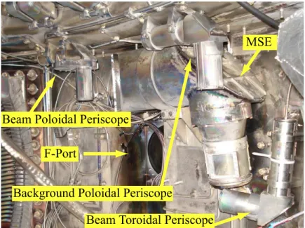
Figure 2-1: View of the outer wall of Alcator C-Mod showing both toroidal and poloidal beam viewing periscopes. Also shown is the MSE diagnostic and the back-ground poloidal periscope. [19]

midplane in the region of the pedestal (0.84 < R < 0.91 cm for C-Mod). At the low-field side (LFS) of the tokamak there are two periscopes, one poloidal and one mostly toroidal, each viewing perpendicular to the path of the diagnostic neutral beam. There is also a poloidally viewing periscope offset toroidally away from the beam to track the background plasma emission. Figure 2-1 shows the outer wall of the tokamak near F-port and all the diagnostics located there. At the high-field side (HFS) there is a single periscope housing several fiber arrays which view parallel to the magnetic field in normal operation. All the periscopes use a single mirror and two lenses (achromats) to focus light onto high-OH silica-clad silica (SCS) fibers with diameters of 400/440/480 µm for the core, cladding, and buffer, respectively.

2.1.1

Low-field side imaging systems

The toroidally viewing periscope at the low-field side is positioned slightly off the midplane to accommodate the MSE diagnostic. This forces the periscope to view

roughly perpendicular to the path of the DNB from an angle of 7.6◦ below the mid-plane. Due to the toroidal tilt of the DNB, the central ray of the views makes an angle of ∼9◦_{with the perpendicular of the path of the DNB when viewed from above.}

A top-down sketch of F-port including the path of the beam and the lines-of-sight of the toroidal periscope can be seen in Figure 2-2(a). For a plasma with a safety factor3

of q95 ∼ 4, the central ray of the periscope makes an angle with the magnetic field

of ∼17◦_{. The periscope optics are protected from all but the most direct particles}

by a black-passivated cylinder, about 9 cm in length. The row of twenty fibers at the image plane of the periscope optics corresponds to a 5 cm range at the midplane with a spot size of 2.2 mm and a radial resolution of 2.7 mm. During typical plasma operation, this provides an estimated radial coverage of 0.75 . r/a . 1.1 (impact radii at the midplane), which includes all of the pedestal region and a portion of both the core (r/a . 0.8) and scrape-off layer (SOL, r/a > 1). The periscope was designed to have its central chord tangent to the flux surface at a major radius of R = 88.6 cm and focus both vertically and toroidally4 in the middle of the DNB. It was determined that several toroidal viewing chords terminated on one of the ICRF antennas, which unfortunately allowed reflections to be collected and distorted the spectra on these channels. This effect makes passive analysis unreliable and completely removes the possibility that a background toroidal periscope could be used for comparison, at least for those channels.

The second periscope is positioned above the beam to view the plasma in a purely poloidal direction. The optics focus plasma light from the midplane onto 25 fibers which have a corresponding spot size at the plasma focus of 2 mm and a radial resolution of 2.4 mm. (Line-of-sight effects through the beam increase this to an

3

The safety factor is the ratio of the number of toroidal rotations for a full poloidal rotation of the magnetic field. q95 is this value at the flux surface which contains 95% of the normalized flux,

relative to that at the LCFS.

4

It was found that the actual focus falls toroidally short of the center of the DNB by ∼5 mm. However, this only affects brightness calculations through the assumed beam characteristics at the focus location.

effective resolution of 3.5 mm.) This periscope covers a 5.5 cm range of the plasma corresponding to 0.7 . r/a . 1.05, similar to the toroidal periscope. The poloidal periscope is aligned with the path of the DNB so that the central ray is vertical to within a tenth of a degree both toroidally and radially. Thus, the line-of-sight from either end of the array is displaced off the vertical by ∼4◦_{. Figure 2-2(b) shows how}

the sight for the poloidal periscope traverse the beam path. The lines-of-sight terminate on a “viewing dump” of black passivated shimstock to avoid stray reflections being collected and distorting the spectra. The toroidal tilt of the DNB in 2006 shifted the alignment of the beam away from the original periscope views, which were aligned along a major radius. Even after a redesign of the mounting plate, it was not possible to perfectly align the array of focal points with the new DNB path. The locations of the views at the midplane deviate from the beam path by 5◦ _on

either side of the central view and are thus no longer aligned with a major radius. Figure 2-3 shows the relative angles between the DNB and the locations of the foci from the toroidal and poloidal periscopes at the midplane. A glass shutter protects the periscope optics from becoming coated with a signal-degrading boron layer during boronization of the machine. This shutter can be manually opened or closed via an external set of pistons.

The final periscope at the low-field side is displaced toroidally from the DNB to provide a simultaneous measurement of the background plasma (i.e., not enhanced by charge-exchange with the DNB). Though originally intended as a background toroidal periscope it was found that reflections off a nearby antenna array invalidated the bulk of measurements made while in this configuration. Before the 2008 run campaign, this periscope was redesigned and repurposed as a background poloidal periscope. Similar to the toroidal periscope, the background poloidal periscope has twenty views, a viewing range of 5 cm, and a spot size of 2.2 mm at the midplane. During normal operation, this covers a range of 0.8 < r/a < 1.03 which overlaps most of the region seen by the poloidal beam-viewing periscope. A black-passivated

F-Port

DNB

Inner Wall Magnetic Axis

Toroidal Periscope Views Focal Points

Magnetic Flux Surfaces

-40 -20 0 20 40 X (cm) Y (cm) 40 60 80 100 120

(a) Top-down view

0.4 0.6 0.8 1.0 R (m) -0.6 -0.4 -0.2 0.0 0.2 0.4 0.6 Z (m) Poloidal Views Focal Points Beam 5.5 cm range (b) Cross-section

Figure 2-2: Schematics of a) the toroidal periscope views with the 6.6◦ _{tilt to the}

DNB shown and b) the poloidal periscope views with the 1/e vertical width of the beam shown. [19]

steel plate provides a viewing dump for this periscope. There is no shutter for this periscope, but a 9 cm long cylinder, similar to the one on the toroidal periscope, protects it from potentially incident particles. As discussed further in section 2.3 below, this background periscope is intended to make it possible to run the DNB continuously (not pulsed) during a discharge. However, it was still optimal to utilize a pulsed beam for the entire 2008 campaign.

2.1.2

High-field side imaging system

At the high-field side of the plasma, the CXRS diagnostic utilizes a capillary tube to inject a small amount of neutral gas into the region of interest. This alternate neutral injection scheme is necessary because even at low densities, the DNB is almost fully attenuated before it reaches the high-field side of the plasma. The magnitude of the injection can be controlled via the pressure of D2 gas in the NINJA and the duration

Figure 2-3: Closer view of the intersection of the DNB and the focal arrays of the toroidal and poloidal periscopes. X = 0 corresponds to the toroidal center of F-port. [19]

that the valve leading to the capillary is open. D2 gas is injected into a discharge

where it quickly disassociates into neutral deuterium atoms that charge-exchange with the local B5+ _{population. Thus, there is an increased probability that}

fully-stripped boron will charge-exchange in a region localized to the midplane near the inner wall. The radial extent of the neutrals from this puff is much smaller than that of the DNB at the LFS, making the range of intersection of fully stripped boron and injected neutrals rather limited. The standard practice is to inject ∼4 torr-L of gas, an amount which yields a density increment similar to the local pre-puff density at the edge of the plasma. For most plasmas, this is not enough to significantly affect the line average densities in the core. A precise measurement of the density of neutrals after injection is not available to us, but a rough estimate can be made from the change in pressure in the NINJA. The enhanced CXRS signal from the puff will persist over several hundred milliseconds and a second puff can be triggered later in the shot to

refresh the neutral population. Through visible imaging of the emission from injected D2 (Dα, 656 nm) the vertical extent of the neutral cloud has been estimated to be

only a few centimeters.

There is a single periscope dedicated to the study of the high-field region near the capillary that is located at the midplane in the inner wall across from B-port. The periscope views down toward the midplane at an angle (10◦_{) designed to make the}

lines-of-sight parallel with the magnetic field of a discharge with a safety factor of q95 ∼ 4. Figure 2-4(a) provides a top-down view of the tokamak near K-port where

the HFS periscope views toward the gas puff injected at the inner wall near B-port. Mounted on the outer wall of the tokamak, the periscope is designed to view tangent to flux surfaces at the toroidal location of the HFS gas puff and perpendicular to the gas puff direction. The lines-of-sight pass through the outer edge of the plasma, intersect the gas puff at the HFS, and then travel through the outer edge again on the other side. Thus, the passive (no puff) signal is composed of emissions from three separate regions along the line-of-sight, but the active (with puff) signal is dominated by the emission from the region near the inner wall.

Light collected by the HFS periscope is imaged onto three parallel arrays consisting of seven fibers each. Figure 2-4(b) shows the relative positions of the three fiber arrays included in the HFS periscope. The fibers have a corresponding spot size in the region of the gas puff of 3.8 mm with ∼4 mm resolution (equivalent to ∼3 mm spacing at the LFS when mapped along the flux surfaces). These arrays view 2.4 cm of the plasma covering only 0.92 . r/a . 1.04 which is often, but not always, sufficient to reach the top of the pedestal. Two fiber arrays collect light from the region at the midplane where the capillary injects neutral gas. Of these two arrays, one is used for CXRS measurements while the other is available to other diagnostics, such as the gas puff imaging (GPI) system for turbulence studies [7]. The third array is vertically displaced from the other two by nearly 4 cm in the plasma. It views above the injected neutral cloud and serves as a measure of the background plasma

Outboard-viewing periscope

Gas puffs

Inboard-viewing periscope: 7x3-fiber array

Last closed flux surface Last closed flux surface K B C A J H

(a) Top down view

CXRS Background Views Capillary Inner Wall Broken fiber GPI views CXRS Signal views (b) Cross-section

Figure 2-4: a) Schematic of the HFS periscope viewing path as it traverses the plasma to intersect the puff. Also shown are the locations of nearby midplane capillaries and a LFS periscope (primarily utilized in GPI turbulence studies). b) Cross-section near the inner wall showing the poloidal separation of the viewing arrays.

light. These background views are also slightly shifted radially in to the plasma to compensate for the curvature of the flux surfaces.

2.2

External components

The CXRS signal is collected by the periscope optics inside the vessel and then relayed to the spectrometers via bundled 400 µm high-OH SCS fibers. The spectrometers disperse the light by wavelength and focus the resulting spectra onto digital cameras. After a complete integration time the collected signal is transferred for processing while light is prevented from falling on the camera. Once the transfer completes the light is again allowed to enter the camera and the new frame of data begins. At the end of a discharge all the frames of data are stored for later analysis.

2.2.1

Spectrometers

The spectrometers used in this research are compact high-throughput (f/1.8) devices made by Kaiser Optical Systems [40]. A volume phase holographic GRISM (grating-prism) disperses the incident light by wavelength, redirecting it by 90◦ _{in the process.}

The fixed-wavelength high-density grating is constructed specifically for light near 494.3 nm and has a transmission of ∼80% at this wavelength. A schematic for the spectrometer and camera system can be found in Figure 2-5. Before entering the spectrometer, light passes through a fixed slit, the width of which determines the spectral width of the instrumental response function. The smallest slit that still allowed sufficient signal to be collected was found to be 100 µm. An 85 mm (f/1.8) camera lens directs the signal into the dispersion grating and a 58 mm (f/1.2) lens focuses it again onto the camera, reducing the fiber image size by a factor of 0.68. A narrow bandpass filter constructed by Barr Associates, Inc. [41] limits the signal to a 3 nm band around the wavelength of interest (494.467 nm). The transmission of the filter is about 90% in the region of interest and quickly falls to less than 10−4

outside this region. This allows multiple spectra to be imaged on a single row of the camera without overlap or interference. Light from fifty-four individual fibers enters the spectrometer in an 18 row by 3 slit configuration. These columns are not vertical but rather follow an arc as seen in Figure 2-5. This compensates for the off-axis light-bending effect of the dispersion grating and allows the exiting spectra to align vertically. A second spectrometer of identical construction allows for a total of 108 channels to be imaged simultaneously.

2.2.2

Cameras

The light from the spectrometers is collected with 16-bit, frame-transfer, Photon-MAX:512B cameras from Princeton Instruments [42]. These cameras utilize a 512 × 1048 16 µm pixel charge coupled device (CCD) which is kept at an optimal temper-ature of -70◦_{C to reduce electronic noise. Figure 2-6 shows a photo of the camera,}

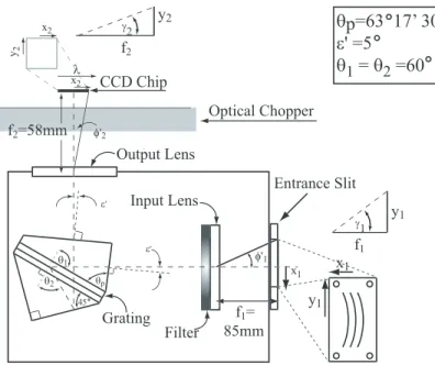
Entrance Slit Input Lens ff22 ffff =58mm=58mm Output Lens Filter CCD Chip Optical Chopper Grating θ1 θ2 θp 45 ε' ε' φ φ''₂ λ λ x2 x2 y2 f f f1 f f = 85mm φ'1 x₁ xx11 y1 y1 f1 ff γ₁ y2 f2 ff γ₂ θp=63 17’ 30” ε' =5 θ₁ = θ₂ =60

Figure 2-5: Schematic of the entrance slits, filter, spectrometer, and camera used to disperse and then digitize the CXRS signal.

chopper housing (discussed below) and the spectrometer. In frame-transfer operation, half of this CCD (512 × 512 pixels) is exposed to light for the prescribed integration time. This “frame” of data is then rapidly transferred down to the other half of the CCD, which is optically masked, at a rate of 600 ns/row. While the lower half of the CCD digitizes the previous frame, the upper half collects new signal, minimizing the time lost to the transfer and digitization process. However, this means that only 512 of the rows are available for imaging during normal operation.

A faster data-taking mode, “kinetics” mode, is also available, wherein all 1048 rows are utilized, but only a small portion of the CCD is illuminated. After a brief integration period (on the order of 100–500 µs) the signal from the exposed region is transferred down the CCD by only the number of rows needed to move that signal out of the illuminated section. This process is repeated until the CCD is full and the whole time history is digitized. Though able to provide much faster temporal resolution of the plasma, the signal-to-noise ratio was prohibitively low when using this alternate method.

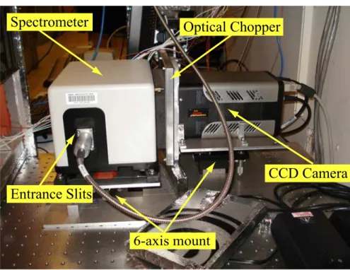
Figure 2-6: Photo of the camera and spectrometer housing. Also shown are the chopper housing and the translational and rotational mounts used for alignment and focus. [19]

The PhotonMAX camera is controlled by the WinSpec program (and related computer hardware) available from Princeton Instruments. All relevant triggering and data taking parameters can be set via the WinSpec interface and the resultant spectra displayed. Furthermore, one may interface with the WinSpec program via any programming language such as C++ or Visual Basic, allowing automation of data taking processes. The WinSpec program has the capability to combine (or “bin”) user defined sections (“regions of interest”) of the CCD before digitization. Each digitization adds an amount of electronic noise to the signal and by combining all the rows corresponding to a specific fiber before digitization we increase the signal-to-noise ratio. Each camera / spectrometer has a dedicated computer to run WinSpec and a custom Visual Basic program which recognizes the initiation of the discharge process, prepares the WinSpec program to take data, and stores the data after it is taken.

2.2.3

Choppers and chopper control

The standard operating scheme for the CXRS diagnostic consists of 5 ms of signal integration with another 1.4 ms “blocking window” in which the frame transfer, which takes ∼0.3 ms, must occur. Even with the rapid shift time (600 ns/row) of the Pho-tonMAX camera, it was decided that blocking the incident light during the transfer was necessary to eliminate the stray light being collected as the data transferred past continuously illuminated rows. To achieve this optical blocking, a chopper system, based on the design by R. Bell of PPPL, was installed between the camera and the spectrometer. This chopper system consists of a dual-tabbed wheel driven by Boston Scientific 300M motor which prevents light from reaching the CCD while the tab is in (or “chopping”) the beamline from the spectrometer. A Boston Scientific Model 300CD controller and synchronizer is used to provide small adjustments (using an optical sensor for feedback) to the chopper motor to keep it blocking the light at the exact time that the camera is transferring the frame. Because of jitter in the chopper speed and thus in the chopper timing, the blocking time was chosen to be substantially larger than the frame transfer time. Unfortunately, the addition of the chopper system requires the design and manufacture of chopper wheels for every tim-ing scheme desired. For example, three-tab chopper wheels that allowed for a 3 ms integration time were manufactured and tested, but these wheels had unexpected jitter problems at the required rotation speed. All the data presented in this thesis was obtained using the standard timing described above.

2.2.4

CPLD system and the A/D Digitizer

To synchronize the two cameras and the two chopper systems with the discharge tim-ing, a custom CPLD (complex programmable logic device) system was developed by W. Burke of the Alcator engineering group. Its limited logic adjusts the chopper spin frequency before the start of the plasma so that individual CXRS time frames may be aligned with planned events during the discharge, such as RF heating or DNB pulses.

This system also provides the cameras with the signals that trigger the frame-transfer process. Output signals from the cameras, choppers, and timing/trigger clocks are all digitized and recorded on a Data Translation (DT9816) A/D digitizer [43]. This allows precise measurement of integration times and verification of chopper control. The DT9816 is capable of digitizing six signals simultaneously and is externally-clocked with a signal generated by the CPLD to prevent phasing between multiple clock sources. Further information on the CPLD, A/D digitizer, and other chopper considerations may be found in Appendix A.

2.3

Spectral Analysis

Once the data are stored, each of the eighteen bins from each time frame are split into three individual spectra and analyzed. Included in these spectra are two emission lines of interest from boron, B V and B II. These lines may be seen in Figure 2-7 which displays spectra from both the high- and low-field sides. The B II line at 494.038 nm is from simple excitation of singly-ionized boron found near the walls of the tokamak. The B V emission (rest wavelength of 494.467 nm) is from the charge-exchange dominated n = 7 → 6 transition of B4+_{. However, because charge-exchange}

is a non-perturbative process and relaxation occurs faster than the ion can equilibrate, the emitting ion still has the characteristics of the B5+ _{(fully-stripped) population.}

The inherent charge-exchange and excitation of B4+ that occurs naturally in the plasma without the addition of neutrals is not localized and must be accounted for as “background” light when analyzing active CXRS spectra. Also found in the collected spectra are weaker lines from various elements which, except for the n = 11 → 8 line (also from B4+_{) near 495.0 nm [44], are ignored during analysis. Unless otherwise}

noted, the term “width” will refer to the full width at half maximum (FWHM) of a spectral line.

4930

4940

4950

4960

Wavelength (A)

0

1

2

3

4

5

6

Counts (

10

3

)

a) HFS

R = 45.77 cm

4940

4950

4960

Wavelength (A)

b) LFS

R = 88.05 cm

B V

B II

B V

B II

Figure 2-7: Example spectra from a) the high-field side pedestal region and b) the low-field side pedestal region. The Zeeman splitting can clearly be seen in the B II line at the HFS. Additional emission lines from other impurities contaminate the LFS spectrum.

2.3.1

Calibrations

Before analysis can begin, several calibrations must be made. These include the calibrations of the wavelength and dispersion for each imaged fiber on the CCD, the radial positions of the views in the plasma, and the transmissions of the collection and relay optics.

Wavelength

The most important calibration necessary for the proper analysis of CXRS data is the wavelength position and dispersion across the camera. Our calibration relies on neon (Ne) lamps (we use those from Avantes, Inc.) which are found to have sufficient line

Figure 2-8: Example fit to neon spectrum for wavelength calibration. The two spectral lines are fit with the sum of three gaussians to generate an instrumental function for this region of the camera. The wavelength dispersion is determined by the distance between the centers-of-mass of the two lines.

strength to do a proper calibration. The relevant Ne spectrum is composed of two lines of equal strength bounding the region of interest at 4939.04 and 494.499 nm. By fitting these two lines, we simultaneously determine the instrumental function and wavelength dispersion for that specific region of the CCD. An efficient method for making instrumental functions is to fit both lines with three gaussians each. The fit-ting routine forces the relative heights, positions, and widths of these three gaussians to be the same for each spectral line. Using three gaussians allows enough flexibility to fit a complex lineshape without becoming computationally intensive. The center of mass of the three gaussians is then taken as the rest wavelength of the Ne line. This process is illustrated in Figure 2-8. The dispersion for the spectrometer and camera system is typically between 0.024–0.026 nm per pixel.

The accuracy of the focus of the image on the camera will also affect the wavelength and brightness calibrations. In order to accurately position the center of the CCD in