Adaptive control of a generic hypersonic vehicle

Adaptive Control of a Generic Hypersonic Vehicle

by

Daniel Philip Wiese

B.S. University of California, Davis (2011)

Submitted to the Department of Mechanical Engineering

in partial fulfillment of the requirements for the degree of

Master of Science

at the

MASSACHUSETTS INSTITUTE OF TECHNOLOGY

ARCHN

Es

JUN 2 5 2013

LIBPARIES

June 2013

©

Massachusetts Institute of Technology 2013. All rights reserved.

A uthor ...

...

Department of Mechanical Engineering

May 10, 2013

Certified by ...

....

.... ..

....

...

. . . . .

Anuradha M. Annaswamy

Senior Research Scientist

Thesis Supervisor

Accepted by ...

David E. Hardt

Chairman, Department Committee on Graduate Students

Adaptive Control of a Generic Hypersonic Vehicle

by

Daniel Philip Wiese

Submitted to the Department of Mechanical Engineering on May 10, 2013, in partial fulfillment of the

requirements for the degree of Master of Science

Abstract

This thesis presents a an adaptive augmented, gain-scheduled baseline LQR-PI controller applied to the Road Runner six-degree-of-freedom generic hypersonic vehicle model. Un-certainty in control effectiveness, longitudinal center of gravity location, and aerodynamic coefficients are introduced in the model, as well as sensor bias and noise, and input time de-lays. The performance of the baseline controller is compared to the same design augmented with one of two different model-reference adaptive controllers: a classical open-loop reference model design, and modified closed-loop reference model design. Both adaptive controllers show improved command tracking and stability over the baseline controller when subject to these uncertainties. The closed-loop reference model controller offers the best performance, tolerating a reduced control effectiveness of 50%, rearward center of gravity shift of -0.9 to

-1.6 feet (6-11% of vehicle length), aerodynamic coefficient uncertainty scaled 4x the

nom-inal value, and sensor bias of +1.6 degrees on sideslip angle measurement. The closed-loop reference model adaptive controller maintains at least 73% of the delay margin provided by the robust baseline design, tolerating input time delays of between 18-46 ms during 3 degree angle of attack doublet, and 80 degree roll step commands.

Thesis Supervisor: Anuradha M. Annaswamy Title: Senior Research Scientist

Acknowledgments

I would like to thank my advisor Dr. Anuradha Annaswamy for her guidance during this research. I would also like to thank Dr. Jonathan Muse and Dr. Michael Bolender in the Aerospace Systems Directorate at the Air Force Research Laboratory for providing the vehicle model for this research, giving their support and advice along the way, and providing direction during my summer work at AFRL. Thanks to Dr. Eugene Lavretsky of Boeing Research & Technology for contributing his invaluable advice and suggestions throughout this project. Thanks also to all of my lab mates for our discussions and help through various research problems, and making lab enjoyable. Their assistance and friendship over the last two years has been great. I also want to thank Dr. Lutz, without whom I would not be where I am today. I want to thank her for all of the encouragement and inspiration over the past five years, and for being a truly outstanding mentor. Thanks as well to Bob for providing advice and wisdom. I would like to thank all of my friends for their patience and understanding. Finally, I would like to thank my Mom, Dad, and all of my family for their love and support all these years.

This research is funded by the Air Force Research Laboratory/Aerospace Systems Di-rectorate grant FA 8650-07-2-3744 for the Michigan/AFRL Collaborative Center in Control

Contents

1 Introduction 15

1.1 Background . . . . 15

1.2 H istory . . . . 17

1.3 Control Design . . . . 21

1.3.1 Need for Adaptive Control . . . . 22

1.4 Overview. . . . . 23

2 Hypersonic Vehicle Model 25 2.1 Modeling the GHV . . . . 26

2.1.1 Equations of Motion . . . . 28

2.2 State Space Representation . . . . 33

2.2.1 Actuator and Sensor Models . . . . 34

2.2.2 Implementation . . . . 36

2.3 Open-Loop Analysis . . . . 36

2.3.1 Modal Analysis . . . . 39

2.3.2 Summary of Flight Modes . . . . 43

2.4 Uncertainties . . . . 45

2.4.1 Representation of Uncertainties . . . . 47

3 Controller Design 49 3.1 Baseline Control Architecture . . . . 50

3.2.1 The Different Loop Transfer Functions . . . .

3.2.2 Closing Inner Flight Control Loops . . . .

3.2.3 Gain Scheduling . . . .

3.3 Adaptive Control Design . . . .

3.3.1 Classical Model-Reference Adaptive Controller . . .

3.3.2 Closed-Loop Model-Reference Adaptive Controller .

3.3.3 The Projection Operator . . . .

4 Simulation Results

4.1 Additional Uncertainties . . . . 4.2 R esults . . . . 4.2.1 Task 1: Angle of Attack Doublet . . . .

4.2.2 Task 2: Roll Step . . . .

4.2.3 Time Delay Margins . . . .

4.3 Summary . . . .

5 Conclusions and Future Work

5.1 Control Performance During Unstart 5.1.1 Unstart Model . . . . A Figures ... ... 54 . . . . 59 . . . . 65 . . . . 68 . . . . 70 . . . . 74 . . . . 76 79 . . . . 79 . . . . 81 . . . . 82 . . . . 84 . . . . 87 . . . . 88 89 89 90 93

List of Figures

1-1 North American X-15 ... ... 19

1-2 NASA X-43A . . . . 20

1-3 Boeing X-51 waverider . . . . 21

2-1 AFRL Road Runner generic hypersonic vehicle [45] . . . . 25

2-2 Reference frames . . . . 29

2-3 Equation of motion model blocks [22] . . . . 33

2-4 Second order actuator block diagram . . . . 35

2-5 GHV flight control simulation block diagram . . . . 36

2-6 Open-loop poles of A for M = 6, h = 80,000 ft steady, level cruise . . . . . 44

2-7 Uncertainty in control effectiveness due to control surface damage . . . . 46

3-1 Inner loop flight control block diagram . . . . 50

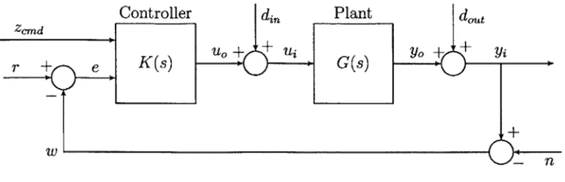
3-2 General MIMO feedback control block diagram . . . . 54

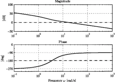
3-3 Velocity loop transfer function Bode plot . . . . 60

3-4 Velocity loop transfer function singular values . . . . 60

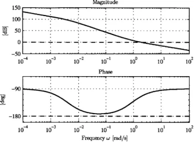
3-5 Longitudinal loop transfer function Bode plot . . . . 61

3-6 Longitudinal loop transfer function singular values . . . . 62

3-7 Lateral loop transfer matrix singular values . . . . 64

3-8 Plot of different trim points with dynamic pressure . . . . 66

3-9 Gain and phase margin of closed-loop subsystems with gain scheduling . . . 67 3-10 Gain and phase margin of closed-loop subsystems without gain scheduling . 67

3-11 Baseline plus adaptive control block diagram . . . . 69

3-12 Classical model-reference adaptive control architecture . . . . 71

3-13 Closed loop reference model adaptive control architecture . . . . 75

3-14 The projection operator . . . . 77

4-1 Simulation block diagram . . . . 79

4-2 State measurements before and after navigation filter . . . . 80

4-3 1A: 50% control surface effectiveness on all surfaces . . . . 82

4-4 IB: Longitudinal CG shift: -0.9 ft rearward . . . . 83

4-5 IC: Pitching moment coefficient Cm. scaled 4x . . . . 83

4-6 ID: Sensor bias of

+1.6

4-7 2A: 50% control surface effectiveness on all surfaces . . . . 84

4-8 2B: Longitudinal CG shift: -1.6 ft rearward . . . . 85

4-9 2C: Pitching moment coefficient Cm. scaled 4x . . . . 85

4-10 2D: Sensor bias of

+1.6

5-1 Ellipses defining region of started engine operation . . . . 90

5-2 Closed loop system block diagram with unstart model . . . . 91

A-1 1A: State response for reduced control surface effectiveness: 50% on all surfaces 94 A-2 1A: Input response for reduced control surface effectiveness: 50% on all surfaces 95 A-3 1B: State response for longitudinal CG shift: -0.9 ft rearward . . . . 96

A-4 1B: Input response for longitudinal CG shift: -0.9 ft rearward . . . . 97

A-5 IC: State response for pitching moment coefficient scaled 4x . . . . 98

A-6 IC: Input response for pitching moment coefficient scaled 4x . . . . 99

A-7 ID: State response for sensor bias of

+1.6

+1.6

A-10 2A: Input response with 50% control surface effectiveness on all surfaces . . . 103

A-12 2B: State response with longitudinal CG shift: -1.6 ft rearward . . . 105 A-13 2C: State response for pitching moment coefficient scaled 4x . . . . 106

A-14 2C: Input response for pitching moment coefficient scaled 4x . . . 107

A-15 2D: State response for sensor bias of

+1.6

+1.6

List of Tables

2.1 Vehicle properties . . .

Second order aerodynamic control surface actuator parameters Sensitivity matrix: nominal flight condition . . . . Sensitivity matrix: nominal flight condition . . . . Velocity controller LQR weights . . . .

Longitudinal controller LQR weights . . . .

Lateral controller LQR weights . . . .

Loop transfer function crossover frequencies Subsystem order . . . .

Subsystem robustness margins . . . . 4.1 Noise variance

Components of trim state vector at nominal flight condition of Mach 6 Delay margins for selected responses in milliseconds . . . .

. . . . 26 2.2 2.3 2.4 3.1 3.2 3.3 3.4 3.5 3.6 35 42 43 4.2 4.3 . . . . 6 1 . . . . 63 . . . . 63 . . . . 65 . . . . 65 . . . . 65 . . . . 80 82 87

Chapter 1

Introduction

1.1

Background

With a history spanning well over a half century, hypersonic flight continues to be a topic of significant research interest [42, 26, 30, 19, 11]. Air-breathing hypersonic vehicles are particularly attractive due to their potential to serve as high speed passenger transports and long range weapon delivery systems, and provide cost-effective access to space. Hy-personic vehicles are likely to be inherently unstable [36, 37, 81 and the integration of the airframe and engine in an air-breathing hypersonic vehicle contributes to additional model-ing and control challenges. With limited wind tunnel data, harsh and uncertain operatmodel-ing environments, poorly known physical models, and largely varying operating conditions, it is of great importance to ensure that any control scheme will be significantly robust to ensure safe operation during flight.

Unlike the transition from subsonic to supersonic flow, the physics of hypersonic flow do not differ from that of supersonic flow. Instead, the distinction of hypersonic flow is made to stress the importance of certain physical phenomena which exist in all supersonic flows that become dominant at hypersonic speeds, typically defined to be flow at a Mach number of 5 or greater [2]. It wasn't until 1946, well into the study of such flow regimes, that this term was finally coined [51]. The high flight Mach numbers experienced by a hypersonic vehicle result in significant aerodynamic heating. This aerodynamic heating can have a great impact

on the material properties of the vehicle. In addition to this coupling of aerodynamic and structural effects, the engines of air-breathing hypersonic vehicles are tightly integrated into the airframe of the vehicle, where long fore and aft sections of the vehicle make up large portions of the engine inlet and nozzle, respectively. This tightly couples the engine dynamics with the airframe and structural dynamics as well as the aerodynamics [15]. The physics of hypersonic flow and these resulting interactions between all the components of the vehicle make the control of hypersonic vehicles very challenging.

A major challenge associated with the control of hypersonic vehicles, in addition to the

interactions between airframe, engine, and structural dynamics, is the limited ability to accurately determine the aerodynamics characteristics [34, 47, 14, 16]. With the presence of such tight coupling between all aspects of a hypersonic vehicle, the ability to collect wind tunnel and flight data to study these interactions would be highly useful. However, these tests are very difficult to do, and so much of the knowledge about a hypersonic vehicle's aerodynamics must come from physics-based models. This makes accurate determination of the aerodynamic characteristics very difficult, making the design of a controller more difficult as well.

Another control challenge associated specifically with air breathing hypersonic vehicles is that of engine unstart. Unstart is a phenomenon caused by several factors including thermal choking and insufficient air recovery at the inlet. This ultimately leads to the upstream propagation of the shock train out of the inlet, effectively preventing air from entering the engine due to a standing normal shock in front of the isolator entrance [18]. This causes an abrupt change in the pitching moment, an increase in drag, decrease in lift, loss of thrust, and potentially changes in vehicle yawing and rolling moments as well [10]. If the flight path is such that it requires the GHV to unstart, the control law must be such that it can accommodate these large and sudden changes, thus ensuring stable flight can be maintained through unstart.

With all of the complex interactions between the different aircraft components, and high level of uncertainty in the models, the control of a hypersonic vehicle is very challenging.

These challenges have led to many advances in the design of flight control.

1.2

History

The science of aerodynamics was first invented in the early 1900s by Ludwig Prandtl in Germany. The field of aerodynamics matured considerably over the next half-century, and during World War II, the Germans were beginning to approach hypersonic speeds in labo-ratory wind tunnel tests at Mach 4.4, and with weapons such as the V-2 rocket approaching similar speeds [27]. The hypersonic technology of the United States was substantially be-hind that of the Germans at the time, until the war ended and Wernher von Braun and his team of rocket scientists came to the United States. Just over eleven years after the end of World War II, history was made when the X-2 became the fastest airplane ever, reaching a speed of almost Mach 3.2. Moments after the record was broken, the plane lost control and began tumbling downwards toward Earth, destroying the plane and killing the pilot due to a mechanism known as inertial coupling [41]. This disaster made the consequences of not maintaining stability during high speed flight very real.

The study of hypersonics in the 1950s was also being propelled by the United States' interest in intercontinental ballistic missiles, which began with the X-17 rocket. The accurate guidance of such missiles over long ranges was of particular importance, but it was the challenges associated with significant aerodynamic heating upon atmospheric re-entry that dominated research in this area during this time. The first test of the X-17 took place in 1956 to investigate the re-entry of a hemispherical nose-cone, and reached a speed of Mach 12.4. This research provided valuable information used in the Mercury program, which succeeded in putting the first American in space in 1961. The inherently stable design of the Mercury capsule allowed safe atmospheric re-entry even without an effective control system. While guidance, navigation and control (GNC) challenges of later hypersonic re-entry vehicles were more difficult, the effective control of atmospheric hypersonic vehicles such as the X-2 was a major problem that needed to be solved.

with much of the knowledge gained through research to be used in the development of high performance fighter aircraft of the time. One of the most notable hypersonic airplanes to ever

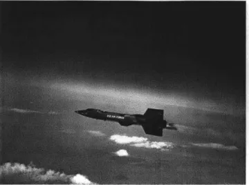
fly, the X-15 pictured in Figure 1-1, made its first flight in 1959. The designers of the X-15

overcame many of the challenges associated with hypersonic flight. The X-15 had to be very heat resistant to withstand the temperatures encountered during flight at nearly Mach 7, and the engine needed the power to propel the plane to these high speeds. The flight envelope of the X-15 was so broad that reaction controls were used in addition to the aerodynamic control surfaces, which lost effectiveness above 100,000 feet altitude. Transitioning between these two control systems was difficult as well. In addition to these challenges, and more, the only significant source of aerodynamic data used in the development of the X-15 came from a single small hypersonic wind tunnel, making modeling for control especially challenging. Despite these challenges, three variants of the X-15 made a combined total of nearly 200 flights over the next ten years following its first flight. The third variant of the X-15, was the only of the three craft to include an adaptive controller as part of its stability augmentation system. This adaptive controller attempted to adjust feedback gains to provide optimum angular rates as commanded by the pilot, and also provided a means to transition from aerodynamic to reaction controls, allowing the command of both control systems from a single control stick in the cockpit. While the X-15 allowed hours of valuable flight data to be obtained, engineers were once again reminded of the consequences of faulty designs when the MH-96 adaptive controller aboard the X-15 failed to reduce the feedback gains upon re-entry, setting up a violent pitch oscillation which destroyed the aircraft and killed the pilot.

Toward the end of the X-15's career, there was a building interest in a new, advanced air-breathing propulsion system for hypersonic flight, as opposed to the rocket propulsion used on the X-15 and its predecessors. This Hypersonic Research Engine (HRE) was to utilize concepts first disclosed by The Johns Hopkins Universities' Applied Physics Lab in 1959, as part of a project known as Supersonic Combustion Ramjet Missle (SCRAM). The scramjet engines were initialy designed as pods, much like conventional turbofans on commercial and

Figure 1-1: North American X-15

transport aircraft. Early plans called for a podded scramjet to be fitted on the X-15, but it

was quickly realized that this would not be possible. To make scramjets practical for use in

flight, the engine would have to be integrated intimately in the airframe, using the fore and

aft sections of the vehicle as part of the inlet and nozzle of the scramjet. Development of

scramjet technology was pushed forward in the early 1980s in part by the U.S. Air Force, in

order to develop a single-stage-to-orbit vehicle to deliver military weapons systems to space.

This ultimately led to the National Aero-Space Plane (NASP) program, and the design of

the 160 foot long Rockwell X-30. This program lasted over ten years and lead to many

advances in scramjet propulsion research and the study of flexible hypersonic vehicles, but

no X-30 were ever built.

Hypersonic research slowed for some years, until scramjet research emerged again in the

early 1990s as part of a collaboration between the United States and Russia. This

collabo-ration saw scramjets mounted aboard rockets being tested in flight. Control again became

a critical challenge in hypersonic flight, this time in the control of the engines. Fuel delivery

had to be controlled precisely to keep the engines operating in supersonic combustion mode,

and avoid a condition known as unstart. Control systems aboard these rocket-mounted

scramjets were designed to monitor pressures within the engines and adjust fuel flow to

Figure 1-2: NASA X-43A

prevent unstart, but the early control systems were not yet ready for this demanding chal-lenges. An all-American effort at practical scramjet powered hypersonic flight was born in

1996 under the name Hyper-X [23]. Hyper-X was an eight year NASA program with the goal

of demonstrating the viability of air-breathing hypersonic flight. The demonstrator vehicle for this program, the X-43, was 12 feet long, and 5 feet wide. The first flight took place in June 2001 and failed, but in March 2004 the X-43A became the first vehicle to ever be propelled during hypersonic flight by an air-breathing engine, reaching a speed of Mach 6.8 for 11 seconds. The third flight in November 2004 lasted 10 seconds and reached a speed of Mach 9.6. These ground breaking flights demonstrated the practicability of a scramjet powered hypersonic vehicle, and are alongside the X-15 in terms of importance in the history of hypersonic flight.

In the 1990s and 2000s, many hypersonics programs have been introduced, including

HyTECH, HyShot, HyCause, HIFiRE, and more. The most notable platform since the

X-43A was the X-51, built by Boeing and managed by the U.S. Air Force Research Lab (AFRL).

While the X-43A demonstrated the feasibility of scramjet powered flight, a new record was set by the X-51 in 2010 by maintaining scramjet powered flight at 5 for 140 seconds. The second X-51 flight took place in 2011 and ended early due to unstart, and during the third test flight the X-51 lost control and fell into the ocean. History was made once again in May

2013, when the X-51 made the longest air-breathing hypersonic flight, maintaining Mach 5.1

for 240 seconds under its own power.

Figure 1-3: Boeing X-51 waverider

The history of hypersonic flight is still in the making, with current research centered around the sustained flight of air-breathing vehicles. The previous trajectories flown by aircraft such as the X-15, X-43 and X-51 were fairly benign in that abrupt and sudden maneuvers were generally avoided, and the goal was to demonstrate primarily the ability of these experimental aircraft to maintain hypersonic flight under their own power. As technology grows the demands of these vehicles will grow too. Current research is being performed to develop new materials and engine designs for these vehicles, as well as advanced control systems which will allow complex maneuvers to be performed while maintaining stability even in situations where unstart conditions are encountered.

1.3

Control Design

Some of the challenges associated with the control of hypersonic vehicles throughout history has been discussed above. These challenges include the limited wind tunnel data available to determine accurate models for control design, large flight envelopes with sig-nificant uncertainty in the operating environment, and need to cope with engine unstart, in addition to problems such as actuator failure, flexibility effects, and time delays. This section discusses some of the existing methods developed to control hypersonic vehicles, and why the adaptive control structure used in this thesis was chosen.

The equations of motion which describe an aircraft are nonlinear, but in most cases it

is acceptable to linearize these equations to facilitate control design and analysis. This lead to the description of aircraft dynamics using the transfer function, and to simple stability

augmentation systems such as roll and yaw dampers [17]. These flight control systems were simple, low-order, linear dynamic feedback compensators such as lead-lag and PID, and

typically used small feedback gains [20, 35, 56]. Thorough frequency domain analysis was

critical to ensure a robust design. Optimal control techniques slowly began seeing use in

flight control in the early 1980s with limited success, but have now become more widely used [13, 1, 50, 49]. Many robust, nonlinear, and adaptive control solutions are proposed in recent literature [55, 24, 29, 28, 9, 44] which include sliding mode, H2/Ho., dynamic inversion, and

neural network control, as well as many other techniques.

1.3.1

Need for Adaptive Control

Adaptive control research was driven in the 1950s by the need for aircraft autopilots

for aircraft that operated in a wide flight envelope, across which the aircraft dynamics

change significantly [3]. While many of the techniques described above offer their own unique

advantages in certain applications, adaptive control is a particularly attractive candidate for dealing with the problems associated with the control of aircraft including hypersonic

vehicles. In order design any controller for a given dynamical system, a model is needed, and with any model there is uncertainty.

Aircraft dynamics can be reasonably approximated by a linearization about a trim flight condition. The parametric uncertainties which are prevalent in aerospace applications such

as control surface ineffectiveness, unknown aerodynamic coefficients, center of gravity shift, and more manifest themselves themselves in a way which is conducive to the design of an adaptive controller. That is, many of the uncertainties associated with hypersonic vehicles

can be represented as parametric ones, entering the system through the control channels.

An adaptive controller can contend easily with these and ensure the desired closed-loop

performance is attained, when degradation of a robust baseline controller is inevitable. The adaptive control structure taken in this thesis is then built around this linearized design

model with the parametric uncertainties. The controller is then applied to the evaluation model, and the efficacy of the controller is examined through simulation studies.

1.4

Overview

Chapter 2 introduces the dynamical equations describing the hypersonic vehicle model. The assumptions used in this model are stated. The equations of motion are linearized about a nominal flight condition, and the flight modes are analyzed. The uncertainties which will be considered, and their representation in the linear model are presented.

Chapter 3 presents the linear baseline control structure which takes advantage of the decoupling of the various flight modes to design three independent control subsystems using state feedback control. Each of the linear controllers is analyzed in the frequency domain to ensure good selection of the feedback gains for fast and robust performance. The process of gain-scheduling this baseline controller across the flight envelope using dynamic pressure is explained. The classical open-loop reference model (ORM), and modified closed-loop reference model (CRM) adaptive control architectures are presented.

Chapter 4 described uncertainties which the model will be subject to within the sim-ulation environment. Simsim-ulation results demonstrating the efficacy of the gain-scheduled baseline and adaptive-augmented baseline controller when the system is subject to various uncertainties are provided.

Chapter 5 provides the conclusions of this research, and describes a simple unstart model which may be used for future research regarding the adaptive control of air-breathing hy-personic vehicles.

Chapter 2

Hypersonic Vehicle Model

The Generic Hypersonic Vehicle which is used as a platform for analysis and control design is shown in Figure 2-1. The Road Runner GHV is a small, pilotless, blended wing-body vehicle, with 3-D inlet and nozzle, and axisymmetric through-flow scramjet engine. There are four aerodynamic control surfaces which can be moved independently, consisting of two elevons and two rudders. The relevant vehicle properties are listed in Table 2.1.

Figure 2-1: AFRL Road Runner generic hypersonic vehicle [45]

hypersonic vehicle model for studies of operability, controllability, and aero-propulsion in-tegration as described in Reference [45]. The objective was to design a common vehicle which would be relevant to the technical efforts of current hypersonic projects, including the

HIFiRE 6 vehicle, which the Road Runner closely resembles, as can be seen in Reference

[9]. _{This GHV was designed be launched on rocket to accelerate it to cruise at Mach 6,}

at a dynamic pressure of between 1000-2000 psf. The mission profile for the GHV then required maneuvers to be performed during the middle of the cruise phase before descending and decelerating, and making an unpowered maneuver to evaluate the potential to make a controlled landing. The GHV should have the capability to perform sustained maneuvers up to a load factor of up to approximately 2G.

Table 2.1: Vehicle properties Parameter Unit Value Gross weight [lbm] 1220.3 Empty weight [lbm] 993.3 Vehicle length [in] 175.9

Span [in] 58.6

Nose diameter [in] 11.0

Tail diameter [in] 18.8

The aerodynamic data for the Road Runner was calculated using Hypersonic Engineering Aerothermodynamic Trajectory Tool Kit (HEAT-TK), developed for the Air Force by Boeing [12], and the engine data is calculated using the Ramjet Performance Analysis (RJPA) code, developed at Johns Hopkins University's Applied Physics Lab.

2.1

Modeling the GHV

The equations of motion describing many aircraft can be derived assuming a flat, non-rotating Earth. Due to the high flight speed of a hypersonic vehicle in the atmosphere, the rotation and curvature of the Earth are typically significant, and should not be neglected.

Thus, the governing equations of motion for the GHV are derived assuming the vehicle is a rigid body flying through the atmosphere of a spherical, rotating Earth. The equations of motion describing the GHV are given in References [22, 6], and will be presented here for completeness.

Notation

In deriving and applying the equations of motion which govern the motion of an aircraft, care must be taken to carefully book-keep the various vector quantities which describe the position, velocity and orientation of the aircraft. For instance, when considering the velocity of an aircraft, it must be kept clear both with which frame the velocity is with respect to, and in which frame the velocity vector is described. Some of the standard notation describing the expression of vectors in various reference frames is outlined below.

*

fa

Q

Oa denotes the origin of reference frame a.

" Vb" describes the velocity of the origin of reference frame b relative to the axes of reference frame a, described using the coordinate system of reference frame b.

* a,b describes the angular velocity of reference frame a relative to reference frame b described using the axes of reference frame c. Omission of the second superscript implies the angular velocity of coordinate system a is with respect to inertial axes. When the subscript is omitted, it is implied this quantity is described in the coordinates of frame a. For example wB is the inertial angular velocity of frame fB, described using the axes of frame fB.

" The transformation Rab describes a vector transformation from being expressed in reference frame b to being expressed in reference frame a.

! d

lb

* All vectors are describing a relation of frame a to frame b are described along the axes of frame a.

In many cases, the equations of motion can be greatly simplified when studying the dynamics of an aircraft. Such simplifications often center around assuming the Earth is flat, but this may be an oversimplification for problems of hypersonic atmospheric flight. While this simplification still might be acceptable for calculations involving the attitude dynamics where the rotating earth terms are typically very small, in trajectory calculations the rotating earth terms for a hypersonic vehicle become non-negligible. This section presents the equations of motion that describe the GHV.

2.1.1

Equations of Motion

The equations of motion are developed using an Earth-centered, Earth-frame fEC with origin at the center of a spherical, rotating Earth. It is assumed that the atmosphere travels uniformly with Earth as it rotates with angular velocity Wearth in inertial space, and that the

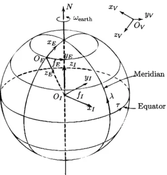
aircraft is sufficiently rigid that flexible structural effects can be neglected. The position of the GHV around Earth and relative to fEC is described by its latitude A, longitude r, and distance from the center of the Earth, g. These three coordinates give the location of the vehicle-carried frame fv, defined with z-axis always pointing toward the origin of

fEc.

The vehicle carrying frame fv is a frame with origin attached to vehicle at the CG, and the z-axis Ovzv is defined to point vertically downward along the local g vector. OVxV is defined to point north, and Ovyv east as shown in Figure 2-2. The vehicle-carried frame has angular velocity wy due to the curvature of the earth. The body-fixed reference frame fB is a right-handed coordinate system attached to the GHV with x-axis pointing towards the nose of the aircraft along the longitudinal axis, and the z-axis pointing down. This body-fixed axis system is used to derive the equations of motion for the GHV.

In deriving the equations of motion, the only additional assumption is that the centripetal acceleration due to Wearth is negligible. The equations of motion describe the dynamics of

the GHV around the Earth when subject to external forces and moments. These forces and moments, given in the body axes by FB, and MB respectively, are due to the thrust and

aerodynamic forces acting on the GHV, and are taken from pre-determined look-up tables within the simulation. The aerodynamic forces depend on on control surface deflection angle,

N xv

Figure 2-2: Reference frames

dynamic pressure, angle of attack, and sideslip angle. The thrust forces depend on on control surface deflection angle, dynamic pressure, and angle of attack.

Force Equations

The force equation describing the the motion of the GHV center of gravity in body axes is given as the following

dV^B

±w9 x Vf +wi x V±w ofx (w x 2)= g±+(FA±+Fr)/m (2.1)

dt A

where VB^ denotes the velocity of fB _{relative to the atmosphere-fixed reference frame, and wEB}

is the inertial angular velocity of the Earth-fixed frame fE, described using the coordinate system of the body reference frame. Note in this work that the atmosphere is assumed fixed with respect to the earth, so fA = fE. The components of the atmospheric velocity are

The force vector EB that represents all non-gravitational forces acting on the body in body axes is given by

FB=[X Y Z

]T

In the Equation (2.1) this force is separated into aerodynamic and propulsive contributions

as FB = FA + FT where the aerodynamic and propulsive forces have components given by

FA=[ XA YA ZA ₍

A Z A ] T(2.4)

FT=[XT

Moment equations

The vehicle moments are described by the following equation. Note the absence of any

rotor contributions to the vehicle moment, as the scramjet engine lacks moving parts, unlike jet-turbine powered craft.

dwB

J + WBXJWB=MA+MT _(2.5)

dt B

WB is the angular velocity of the body frame relative to the inertial frame, with the rate of change evaluated in the body frame, and components

wB

=[ p q

(2.6)

The total torque in body axes is given by

MB=[L

M N

This total moment is split into the contributions due to aerodynamic and propulsive moments

components given by

MA=[LA MA NA]T

(2.8)

MT =[LT MT NT ]T

The moment of inertia matrix J is given by

J

-Jxy

-Jxz

J= JXY JYY -JYZ (2.9)

-Jxz -Jyz Jzz

Without any simplification, expansion of the moment equations would become very cumber-some. In general, aircraft are symmetric about the x - z plane, mass is uniformly distributed, and the body coordinate system is oriented such that Jxy =Jyz = 0. This allows the moment

of inertia matrix for the GHV to be simplified to

JX, 0 - Jxz

J= 0 Jyy 0 (2.10)

-JXz 0

Jzz

Orientation Equations

The orientation, or kinematic equations describe the orientation of the aircraft body axes with respect to the vehicle carried frame. The relationship between Euler rates and body angular velocities in the vehicle- carried frame is given by

[

L

0 sin(4)/ cos(0) cos()/ cos(0) r

where

#,

with body-fixed reference frame fB and are relative to the vehicle-carrying frame fv. These components of angular velocity are about the x, y, and z body axes, respectively. The relative angular velocities of the GHV are related to the vehicle absolute angular velocities by

P[

P

f

q

q

-A

rV r -(Wearxth+

-?)

A

where RBV is the orthogonal rotation matrix given by

cos 0 cos ' cos 0 sin V) -sin 0

RBV = sin

#sin

0

*/

V/

+

#

sin# cos

1

#

+ sin

#

#

#

#

The reason for the distinction between relative and absolute angular rates in the above

equations is due to the spherical Earth. If a hypersonic vehicle was flying continuous circles

around the world, the Euler rate's would all be zero as the aircraft would be stationary

relative to the vehicle carried frame. However, the absolute angular rates would be non-zero,

as the vehicle carried frame would be rotating as it moved over the surface of the Earth.

Navigation Equations

The location, or navigation equations describe the location of the origin of the body fixed coordinate system with respect to the inertial axes. The quantities describing this location are latitude, longitude, and altitude. The navigation kinematic equation is given by

[eR

A

Construction of Equations

These equations were assembled in a SIMULINK model with main component blocks as indicated in Figure 2-3. The forces and moments are calculated from aerodynamic and engine data stored in look-up tables.

'MOnin Eq. p6 q. r -4uF -A Q. R * *~Kanmacs.. 0.0 1 (LI9

->--

(5210z)Fw

Pi

i~

Figure 2-3: Equation of motion model blocks [22]

2.2

State Space Representation

The equations of motion can be represented in state-space form as

X

= f(X, U)

with state vector

x=

V,

0

0

p

#

#,

input vector is given by

U

[

(2.17)

where Uth, Uelv, Uail, and Urud are the throttle, elevator, aileron, and throttle inputs, respec-tively. The entries of the state vector are arranged so as to facilitate separation of the lateral and longitudinal equations of motion during control design. The deflection of the elevons are

accomplished through static mixing, combining differential and collective deflections from

the aileron and elevator commands, respectively, while both rudders are actuated together

using the single rudder input. The control vector U5 contains the deflections of the right and

left elevons (ur,eiv, Ui,eiv), rudders (Ur,rud, U,rud), and throttle as

U5 =

[

]

U

where control allocation matrix is

1 0 0 0 0

M = 0 1/2 1/2 0 0 (2.20)

0 1/2 -1/2 0 0 0 0 0 1/2 1/2

2.2.1

Actuator and Sensor Models

Throttle The propulsion system is modeled as a first order system with a cutoff frequency

of 10 rad/s, with transfer function

Gth(s) = Wth

S + Wth

While the physics of the engine happen on time scales order of magnitude faster than the rest of the dynamics, this simple model was proposed to capture fuel system delivery limits.

Control Surfaces Second order actuators with rate and deflection limits were included in the simulation model on all four of the aerodynamic control surfaces. The transfer function for the control surface actuators is

w2

Gc.(s)

2 2

s2

+2(Wns

and the block diagram for the control surfaces as implemented is shown in Figure 2-4 where the signal Ucmd is generated by the controller, and due to the actuator dynamics the actual control surface deflection is given by usat.

Figure 2-4: Second order actuator block diagram

The relevant values used in the second order aerodynamic control surface actuator model

are listed in Table 2.2.

Table 2.2: Second order aerodynamic Parameter

control Unit

surface actuator parameters Value

Elevon deflection limit [deg] -30 to 30 Tail deflection limit [deg] -30 to 30 Elevon rate limit [deg/s] -100 to 100 Tail rate limit [deg/s] -100 to 100

Damping ratio ( 0.7

Sensor Filters First order low-pass filters were placed at the sensor outputs in order to

model the effects of a navigation filter in the loop, and reduce sensor noise being fed back to the controller. The velocity filter has a cutoff frequency of 20 rad/s, while the incidence,

angular rate, and Euler angle sensor filters all have a cutoff frequency of 150 rad/s.

2.2.2

Implementation

The GHV simulation block diagram is in Figure 2-5. The controller was implemented in discrete time and operated at 100 Hz with a zero-order hold on the control signal output. The output sensors are operated at 600 Hz also using zero-order hold samping, white noise was injected into the sensor signals, and a variable input time delay was used.

noise

Zcmd I

Controller Td% -+ Actuators + ZOH Filter

100 Hz- -- ~~~~

--600 Hz

Figure 2-5: GHV flight control simulation block diagram

The discretization of the controller and sensor models as well as the addition of time delay, actuator dynamics, and noise makes the evaluation model a more realistic representation of the actual hardware on which the proposed control laws would be implemented. This is to better evaluate through simulations the robustness capability of the control design as it contends with these realistic effects.

2.3

Open-Loop Analysis

The open-loop behavior of the GHV was analyzed about a nominal flight condition of

M = 6, h = 80,000 ft, corresponding to a dynamic pressure of 1474 psf. The geographical

coordinates and heading of the GHV are insignificant in the equations of motion for the purposes of inner-loop control law development, and these state variables are dropped from

the state vector (2.16) for trim, linearization, and control.

X=[ VT

a

0 h

3 p r

The state X from this point forward is used to mean the truncated state (2.22), as it contains the primary quantities describing the vehicle dynamics that are to be controlled. The navigation components of (2.16) will evolve as a consequence of controlling (2.22) and in practice would be commanded through an outer-loop guidance controller. The dynamics of the system with truncated state are described by

X =

f(X,

The equilibrium, or trim state Xeq and input Ueq satisfy

Zeq

f(Xeq,

The equilibrium state and input are found for the nominal steady, level cruise condition, and Equation (2.23) is linearized about this trim condition as follows. Defining x and u to be state and input perturbations about equilibrium, the state and input can be expressed as

X = Xeq ± X (2.25) U = _{Ueq + U} Differentiating (2.23) X

= z= f(X, U)

=f(Xeq + X, Ueq + u)

Performing a Taylor series expansion, neglecting second order terms and higher

.

(Xe

eOf(X,

U)

U)

where the subscript (-)eq indicates these quantities be evaluated at the equilibrium point. With f(Xeq, Ueq) = 0, the linearization results in the state-space system given by

=Ax + Bu (2.27)

where

A - Of (X, U)

_ax

B - Of (X, U)

(2.28)

eqau e

eq eq

Using this linear system, the open-loop dynamic modes of the GHV during the nominal steady level cruise condition are analyzed through a sensitivity analysis. It is also impor-tant to note that the perturbation state x of the linear system in Equation (2.27) will be represented as having the following components.

x

Aa

]T

The perturbation input for the linear system is equivalently defined as

u =

]

In following sections, this notation is abused by not explicitly including the A preceding each component to indicate that the components of the state vector x and input vector u are in fact perturbation states and inputs, respectively. This is done only when there is no possibility of confusion, and so when referring to the state and control input of the linear system given by Equation (2.27) the following notation will be used

X=[ VT a

q 0 h /3p

]T

2.3.1

Modal Analysis

Given a linear system such as Equation (2.27) it is often of interest to examine the system modes. Conventional aircraft usually have modes which are quite predictable in their characteristics from one vehicle to the next, but with an aircraft such as the GHV, the significant state variables in the different modes may differ from those of conventional aircraft. Because of this it is crucial to analyze the system modes to better understand the dynamics of the GHV, and to facilitate the control design process.

The sensitivity matrix for the linear system given in Equation (2.27) is calculated, which contains the desired modal information. The sensitivity analysis aims to determine which entries in a given eigenvector are small when the units of each state variable are not the same. This method examines slight changes in the initial condition of each state separately in order to determine whether this change will influence some modes more strongly than others. This analysis will provide knowledge of what modes the GHV exhibits, which states are dominant in each of these modes, as well as the stability of these modes.

Mode Sensitivity

Consider the linear system (2.27) describing the GHV dynamics, with perturbation state vector given by (2.31). This section outlines the method presented in [22] of applying a linear transformation to a state space system to obtain a system represented in characteristic coordinate system to facilitate the modal analysis and calculation of the sensitivity matrix. Considering only the initial condition response, the following autonomous system results

i=Ax (2.33)

The following nonsingular transformation is introduced

where V - [ vi ... v ] is the modal matrix made up of the eigenvectors or A as shown. Note that this transformation will not alter the eigenvalues or eigenvectors of the system in

(2.33). Using this transformation

q=Aq

A= V AV

(2.35)

(2.36)

The matrix V-1 AV can be expressed as

AV

giving

q=Aq

where A is the diagonal matrix of eigenvalues. The solution is given by

q(t) = eAq(o)

(2.37)

(2.38)

(2.39)

The unforced response of the system in response to initial conditions is of interest. particular, an initial condition is selected as a scalar multiple of an eigenvector vi

X(0) = aivi

In

(2.40)

Using the linear transformation

q(0) = V~1x(0) = aiV 1vi (2.41)

Since V-V = R where I is the identity matrix, V-1vi is just the ith column of I. In other words, the initial condition q(0) corresponding to the selected x(0) will be a column vector of zeros, with the exception of the entry a in the ith row. The response of the state x(t) where

from this initial condition is given by x(t) = VeAtaiV-lvi = aiVe^ [ 0 ... 1 ... 0

]

This shows that only the mode corresponding to Ai will be present in the response from an initial condition along the ith eigenvector. The general response in terms of x is given by summing the individual responses starting from each eigenvector initial condition

n

x(t) = aie'vi

Based on this unforced modal response, if any entries in vi are small relative to the others, the corresponding states are thus not influential in determining the initial condition response.

Calculating the Sensitivity Matrix

In this section the methods of [21] used to calculate the sensitivity matrix for A are outlined. The matrix V and its inverse V-' are first calculated. The rows of V are denoted using ri, and the columns of V-1 as ci

V- = C1 C2 --. Cn]

V=[ ri r2 ... rn ] X(t) = ai I ... v- V I

The diagonal matrices Ci are formed using the elements of c ci = c ,1 C ,2 cin

Ci

ci,1

The n x n sensitivity matrix S is defined as

r1

C

= r2C2

Sensitivity Matrix Analysis: Nominal Flight Condition

The sensitivity matrix S is shown in Table 2.3 for a nominal flight condition of flight Mach number M = 6 and altitude h = 80, 000 ft, giving a dynamic pressure of q = 1, 474 psf.

Table 2.3: Sensitivity matrix: nominal flight condition

Al A2 A3 -2.24 -4.87 1.89 A4 A5 1.37 i 0.76j l6 A7 0 ± 0.12j A₈ A9 -0.0039 -0.0272

VT 3.44E-05 1.22E-13 6.57E-05 1.34E-10 1.34E-10 0.0022 0.0022 0.9955 2.46E-09

a 0.3618 7.31E-10 0.3226 3.04E-08 3.04F,08 0.1578 0.1578 3.04E-05 4.96E-10 q 0.4823 1.05E-09 0.5103 4.97E-08 4.97E-08 0.0036 0.0036 2.48E-07 4.57E-12 0 0.0088 1.79E-11 0.0160 3.92E-09 3.92E-09 0.4876 0.4876 5.32E-05 1.59E-09 h 0.0012 9.70E-13 0.0020 5.77E-10 5.77E-10 0.4962 0.4962 0.0044 8.55E-10

# 1.79E-10 0.2311 1.16E-07 0.3844 0.3844 3.17E-11 3.17E-11 3.30E-15 7.59E-05 p 2.81E-09 0.4259 5.66E-08 0.2855 0.2855 7.34E-10 7.34E-10 4.73E-12 0.0031

r 3.87E-10 0.0119 9.56E-09 0.3412 0.3412 7.91E-09 7.91E-09 1.73E-10 0.3058

4 5.01E-11 0.0237 4.84E-08 0.3096 0.3096 1.08E-08 1.08E-08 2.88E-09 0.3570

Each row corresponds to a state, and the modes corresponding to the columns. In each column, the magnitude of the each entry indicates how influential this corresponding state is in the mode corresponding to that column. The values in any given column which are

at least one order of magnitude greater than the other values are shown in bold, showing the states which are most dominant in each mode. The smallest terms, which are several orders of magnitude less than the largest values in each mode do not significantly impact the response. These values are removed, as shown in the sensitivity matrix in Table 2.4.

Table 2.4: Sensitivity matrix: nominal flight condition

A A2 A3 A4 A5 A6 A7 A8 Ag -2.24 -4.87 1.89 1.37 i 0.76j 0 i 0.12j -0.0039 -0.0272 VT - - - - - 0.0022 0.0022 0.9955 -a 0.3618 - 0.3226 - - 0.1578 0.1578 - -q 0.4823 - 0.5103 - - 0.0036 0.0036 - -0 0.0088 - 0.0160 - - 0.4876 0.4876 - -h 0.0012 - 0.0020 - - 0.4962 0.4962 0.0044 -# - 0.2311 - 0.3844 0.3844 - - - -p - 0.4259 - 0.2855 0.2855 - - - 0.0031 r - 0.0119 - 0.3412 0.3412 - - - 0.3058 <p - 0.0237 - 0.3096 0.3096 - - - 0.3570

Table 2.4 shows the influence of the significant states on each mode. From this, it can

be seen that the assumption of decoupled lateral and longitudinal dynamics is a good one.

None of the lateral states are present in any of the longitudinal modes, and none of the

longitudinal states are present in the lateral modes. Comparing the magnitude of the entries

in the sensitivity matrix for the GHV, each of the modes was separated by at least one order of magnitude difference, indicating a strong decoupling of the flight modes.

2.3.2

Summary of Flight Modes

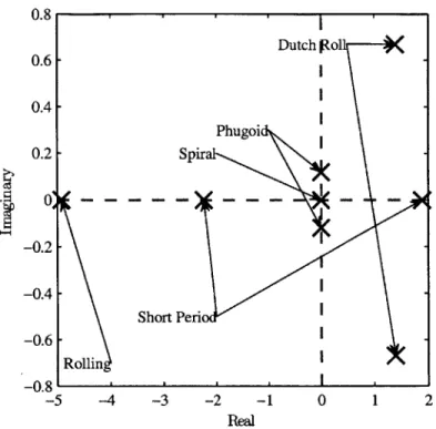
The sensitivity analysis indicated the presence of two longitudinal and three lateral flight

modes as shown in Figure 2-6. The GHV has a highly unstable irregular short period mode

and an unstable dutch roll mode. The phugoid mode is neutrally stable, and the rolling

mode is stable. The velocity mode is given by a pole at the origin, and is omitted from

0.8 0.6 -0.4 -0.2 - Spir Phugoi -0.2 -0.4-Short Peri -0.6-Rollin -0.8 -5 -4 -3 -2 -1 0 1 2 Real

Figure 2-6: Open-loop poles of A for M = 6, h = 80, 000 ft steady, level cruise

The sensitivity analysis performed above indicates the presence of six flight modes. These modes are explained below.

" Short Period (A1,3) -an unstable mode dominated by a and q. Relatively fast, purely

real poles, with A1,3 ~ ±2.

" Rolling (A2) - a stable mode, dominated by

#

" Dutch-Roll (A4,5) - an unstable mode, which is a combination of a rolling, pitching, and yawing motion in flight.

" Phugoid (A6,7) - a neutrally stable phugoid-type mode. " Velocity (A8) -neutrally stable.

" Spiral (A9) - a slow, but stable mode.

The eigenvalues corresponding to the different modes are shown in the pole plot in Figure

the other longitudinal dynamics. This stability analysis was repeated at several other flight conditions, and revealed the same basic modes, although the pole locations and stability of some of the modes differed from the flight condition shown here.

This analysis allowed the velocity, longitudinal, and lateral-directional subsystems to be decoupled, and each of these three plant subsystems to be represented as

ip = Apxp + Bpu (2.44)

where x, E R'P, Ap E Rnp""p, B, E RnPxm and u E R'. Note that these sizes will differ for each of the subsystems.

2.4

Uncertainties

A model is only a mathematical representation of a system or process, and so the

pres-ence of uncertainty in any plant model is inevitable. This is particularly true in the case of a hypersonic vehicles, due in part to engine/airframe coupling, complex shock interac-tions, flexible effects, and unsteady aerodynamics [36, 46, 52]. Many of these uncertainties can be represented as parametric uncertainties as shown in (2.46), and include unknown aerodynamic coefficients and control ineffectiveness, among others.

When building a more conventional vehicle such as a subsonic transport aircraft, much wind tunnel and flight test data is collected, and the aerodynamic coefficients describing the aircraft can in general be determined with a high level of accurately [33, 38]. This data is difficult to obtain for a hypersonic vehicle, where wind tunnel testing is more difficult to do. Additionally an extremely limited amount of hypersonic flight test data has ever been recorded, especially for air-breathing hypersonic vehicles. Existing analytical techniques often fail to accurately predict the stability derivatives for air-breathing vehicles due to hypersonic flow assumptions which are violated due to the presence of the engine [53]. The use of CFD has become increasingly used to model the aerodynamics of hypersonic vehicles, but there is still much work to be done.