A Regionalization of Downscaled GCM Data Considering Geographical Features in a Mountainous Area.

(1)

Research Article

A Regionalization of Downscaled GCM Data Considering

Geographical Features in a Mountainous Area

Soojun Kim,

1

Jaewon Kwak,

2

Hung Soo Kim,

3

Yonsoo Kim,

3

Narae Kang,

3

Seung Jin Hong,

3

and Jongso Lee

3

1_{Columbia Water Center, Columbia University, New York City, NY 10027, USA}

2_{Centre Eau Terre Environment, INRS490, rue de la Couronne, QC, Canada G1K 9A9}

3_{Department of Civil Engineering, Inha University, Nam-Gu, Incheon 402-751, Republic of Korea}

Correspondence should be addressed to Hung Soo Kim; sookim@inha.ac.kr

Received 19 April 2014; Revised 8 August 2014; Accepted 10 August 2014; Published 8 September 2014 Academic Editor: Richard Anyah

Copyright © 2014 Soojun Kim et al. This is an open access article distributed under the Creative Commons Attribution License, which permits unrestricted use, distribution, and reproduction in any medium, provided the original work is properly cited. This study establishes a methodology for the application of downscaled GCM data in a mountainous area having large spatial variations of rainfall and attempts to estimate the change of rainfall characteristics in the future under climate change. The Namhan river basin, which is in the mountainous area of the Korean peninsula, has been chosen as the study area. neural network-simple kriging with varying local means (ANN-SKlm) has been built by combining the artificial neural network, which is one of the general downscaling techniques, with the SKlm regionalization technique, which can reflect the geomorphologic characteristics. The ANN-SKlm technique was compared with the Thiessen technique and the ordinary kriging (OK) technique in the study area and the SKlm technique showed the best results. Future rainfall levels have been predicted by downscaling the data from CNRM-CM3 climate model, which was simulated under the A1B scenario. According to the results of future annual average rainfall by each regionalization technique, the Thiessen and OK techniques underestimated the future rainfall when compared to the ANN-SKlm technique. Therefore this methodology will be very useful for the prediction of future rainfall levels under climate change, most notably in a mountainous area.

1. Introduction

Climate change can affect the spatial and temporal distribu-tions of water resources as well as the intensities and frequen-cies of extreme hydrological events [1]. Climate change causes temperature increases over a long period of time, change in rainfall amounts and patterns, dry spells, and a rise in sea levels. There are many ongoing studies on the evaluation of climate change impacts on water resources such as river flow quantity, water-quality, ecology, groundwater, agriculture, snowmelt, and hydroelectric power generation. The results of these studies are integrated and published by the IPCC in assessment reports [2–6].

One of the important issues for the analysis of climate change impact is the part related to the downscaling of GCM (general circulation model) data. Many researchers

are focusing their efforts on suggesting and improving various downscaling techniques. The studies on downscaling techniques had arisen from the issue on the resolution of GCM. Therefore, the studies on utilizing GCM data from the perspective of hydrology can be largely classified into dynamical and statistical downscaling techniques.

The dynamical downscaling technique is a numerical model based on a computer program that provides vari-ables and fluxes on weather and climate by meteorological equations. Regional climate models (RCMs) and limited area models (LAMs) are the quintessential examples. It is a process of creating weather scenarios through a physical circulation process while having a GCM as the boundary condition

[7, 8]. Since RCMs can simulate the study area in high

resolution, many studies utilized RCMs [9–13]. Many projects that evaluated the impact of climate change and vulnerability Volume 2014, Article ID 473167, 14 pages

(2)

to climate change in limited regions, such as the UK Climate Impacts Programme [14], the Prudence [15–17], the North American Project NARCCAP, and CRES [18], used dynam-ical downscaling technique.

Statistical downscaling techniques use the statistical cor-relation between low resolution GCM and local observed data

[19, 20]. Hanssen-Bauer and Førland [21], Hellstr¨om et al.

[22], and Fowler et al. [10] applied a statistical downscaling technique that used the relationship between atmospheric hydrometeorological variables and rainfall/temperature of the ground surface. Cubasch et al. [23], Kidson and Thomp-son [24], Hanssen-Bauer et al. [25], and Chu et al. [26] also used statistical downscaling techniques by drawing the main components of pressure fields or geographical-potential heights. There are also studies that applied statistical down-scaling techniques, such as the studies using artificial neural networks (ANN), which is mainly used in nonlinear forecast-ing [27–30], and the studies that applied canonical correlation analysis (CCA) [31–37]. Kyoung et al. [38] applied K-nearest neighbors (KNN) as a statistical downscaling technique.

Recently, there are also the comparison studies of dynam-ical downscaling techniques and statistdynam-ical downscaling tech-niques [39–42]. It is possible to understand the strengths and weaknesses of each technique from these papers. Although both statistical and dynamical downscaling methods have their own merits, statistical downscaling is more widely adopted in hydrological studies because it is less computa-tionally demanding [43]. There are some specific reasons why hydrologists have used statistical downscaling for GCM data with the transfer function method. One reason is that it is difficult to directly utilize RCM data on hydrologic analysis without calibrating RCM data. Another reason is that there is a limitation that all information required for future water resources impact evaluation cannot be easily obtained from RCM data. However, when GCM data is used, there is an issue caused by the resolution of GCM. A GCM for which one grid is 300–500 km represents the Korean peninsula by 2–4 grids. Most of the Korean peninsula (about 70%) is mountainous area, which has fairly large spatial deviations in weather phenomena and is strongly affected by geomor-phologic characteristics; therefore, geomorgeomor-phologic charac-teristics should be considered when applying downscaling and regionalizing techniques in mountainous areas. It can be said that general downscaling techniques that downscale GCM data to the locations of weather stations in a basin cannot properly reproduce the weather characteristics of the basin.

Therefore, this study intends to improve the spatial limita-tion of the statistically downscaled GCM data using a region-alization method, which should precede the climate change impact evaluation on water resources in a mountainous area. For this purpose, a methodology accommodating geomor-phologic characteristics will be suggested for the downscaling and regionalization. It will then be analyzed and compared with existing methodologies. Lastly, the change in rainfall characteristics caused by climate change will be examined by forecasting future rainfall, which will be downscaled and regionalized from future weather data by the methodology suggested in this study.

2. Data Used and Methodology

2.1. Climatic Datasets

2.1.1. Observed Climate Data. The Namhan river basin in

Korea has been chosen as the study area because it represents the meteorological and geomorphologic characteristics of the Korean peninsula fairly well and good quality data with a sufficiently long historical period was available. The total area of the Namhan river basin is 12,577 km2 and the length of the river is 375 km. The upstream of the basin belongs to highland with altitudes in the 500 m to 1,700 m range, while the downstream belongs to a hilly area with altitudes ranging from 40 m to 500 m. The data from fifteen weather stations under the jurisdiction of the Korea Meteorological Adminis-tration (KMA) in the Namhan river basin will be used for this study (Figure 1). In addition, the information from 26 rainfall stations in the Namhan river basin under the jurisdiction of the Ministry of Land, Infrastructure, and Transport (MLIT) is collected to examine the applicability of downscaling techniques suggested by this study (Figure 1). In other words, we use rainfall data obtained from fifteen stations of KMA for the evaluation of the SKlm downscaling technique suggested in this study. For the comparison of the SKlm technique with Thiessen and OK techniques, the rainfall data from 26 rainfall stations of MLIT are used. Here the rainfall stations are more densely distributed than the other fifteen weather stations and so spatial accuracy of rainfall by the SKlm technique can be evaluated by the rainfall data from the 26 stations in the basin.

2.1.2. NCEP-NACAR Reanalysis Data. The National Oceanic

and Atmospheric Administration (NOAA), Earth System Research Laboratory (ESRL), Physical Sciences Division (PSD) provides the observed data of 29 global units, including NCEP reanalysis data from their homepage. The NCEP reanalysis data, which is mainly used in studies related to cli-mate change, includes temperature, relative humidity, specific humidity, sea level pressure, evaporation, U-wind, and V-wind observations from January 1, 1948, until now for the time scales of month, day, and every four hours. The monthly NCEP data from 1973 to 2008 for the Korean peninsula was downloaded and is utilized in this study.

2.1.3. Climate Model and Scenario. Kyoung [44] had chosen the BCM2, CNRM-CM3, FGOLS, and MIHR models, which simulate the Korean peninsula as land, not ocean, out of 24 GCM models given by the IPCC Data Distribution Centre (IPCC DDC) on higher priority and examined the appli-cability on the Korean peninsula. He finally suggested that the CNRM-CM3 model is the most appropriate model for the Korean peninsula. Therefore, this study adopted CNRM-CM3 model by referring to the results of Kyoung [44]. This study also selected the A1B scenario suggested by IPCC AR4 [5] because A1B is closest to reality, considering the whole world is trying to maximize energy resource efficiency and find alternative energy sources. There is a paper by Kwon et al. [45] in which the investigators performed their analysis using the A1B scenario.

(3)

Japan China Mongolia Pacific Ocean Korea Weather station Rainfall station Hongchun Yangpyeong Icheon Jecheon Wonju Chungju Daegoanrung Cheonan Chungju Boeun Mungyeong Andong Bonghoa Taebaek Donghae Gebang Russia Imge Dukam Sabook Hadong Danyang Duksan Chungchun Dalcheon Samjuk Yeoju Moonmak Anheung Sinlim Banglim Choondang Bongpyung Hoingsung Chubu Yonduk Stream Subbasin DEM (m) 40.0–191.2 191.2–342.3 342.3–493.5 493.5–644.7 644.7–795.8 795.8–947.0 947.0–1098.2 1098.2–1249.3 1249.3–1400.5 1400.5–1551.7 0 (km)50 100 N S W E

Figure 1: Study area and the location of weather and rainfall stations.

2.2. Methods. This study examines the artificial neural

net-work (ANN) and simple kriging with varying local means (SKlm) technique as a spatial downscaling technique. Recently, many studies suggested the ANN technique, which is a nonlinear model of the data series, and ANN is better than other techniques by way of systematic evaluation of various techniques [27, 28, 46]. Therefore, this study also applies ANN, which is judged to have superior applicability in the simulation of nonlinear characteristics of weather data series. For the spatial distribution of monthly rainfall series in the application of downscaling technique, the kriging technique, which is applied in various areas for a spatial interpolation, is considered. The SKlm technique has been applied as a downscaling technique because it is an improved version of the simple kriging technique, which is capable of spatial inter-polation using geomorphologic characteristics as secondary data.

2.2.1. Spatial Downscaling Technique Using ANN. ANN is a

model of neurotransmission by a neuron, which is a nerve cell in the human brain. ANN is an empirical pattern search technique that enables the consideration of a nonlinear rela-tionship between input variables and output variables. ANN is used in various areas because of its unique applicability

[47,48]. This includes the field of climate science, where its

applicability is proven [49,50].

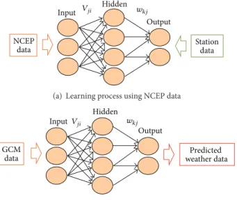
In this study, an ANN model is suggested to apply the downscaling technique through GCM data. The spatial downscaling procedure using the ANN model is summarized as shown inFigure 2.

(1) Select the common factors that can generate desired output values by collecting GCM data, NCEP data, and weather data at weather stations. Create input data for the ANN.

(2) Create hidden layer considering both the input data (NCEP) and output data. Build a network by connected weights and build multilayer perceptron model.

(3) Create objective function from output data and com-parable observed values at weather stations.

(4) Create output data from the connected weights of random seed. Compare it with observed values using the objective function.

(5) Complete the learning by making most optimum connected weights by way of repetitive adjustment of connected weights using error backpropagation algorithm.

(6) Simulate future weather phenomena series by using learned ANN and GCM data as input data.

(4)

NCEP data Station data Vji wkj Input Hidden Output

(a) Learning process using NCEP data

GCM data Predicted weather data Vji wkj Input Hidden Output

(b) Forecasting process using GCM data

Figure 2: Downscaling technique using ANN.

2.2.2. Considering the Influence of Geomorphologic Charac-teristics on Downscaled Rainfall. Kriging is a generic name

adopted by geostatisticians for a family of generalized least-squares regression algorithms. The simple kriging (SK) esti-mate of𝑧(𝑢) is 𝑧∗sk(𝑢) − 𝑚 = 𝑛(𝑢) ∑ 𝛼=1 𝜆sk 𝛼(𝑢) [𝑧 (𝑢𝛼) − 𝑚] , (1) where𝑚 is the stationary mean of 𝑧(𝑢) and 𝜆sk_𝛼 is the weight assigned to datum𝑧(𝑢_𝛼).

Simple kriging with varying local means (SKlm) amounts to replacing the known stationary mean in the SK estimate(1) by known varying means𝑚∗_sk(𝑢) derived from the secondary information [51]. It may be written as

𝑍∗sk(𝑢) − 𝑚∗sk(𝑢) = 𝑛(𝑢) ∑ 𝛼=1𝜆 sk 𝛼 (𝑢) [𝑍 (𝑢𝛼) − 𝑚∗sk(𝑢)] . (2) The characteristic of SKlm is that the local mean(𝑢) of primary data is replaced by the𝑚∗_sk(𝑢) of secondary data.

This methodology can be applied through the following procedures.

(1) Calculate the local means by a regression relationship between the primary data and the secondary data. (2) Calculate the residuals using the relationship between

observed value and local mean. (3) Make a variogram on the residuals.

(4) Estimate residuals for ungauged locations by per-forming kriging on the residuals.

(5) Obtain the estimated values for ungauged locations by adding residuals to the local mean.

3. Model Construction and Estimation of

Future Monthly Rainfall

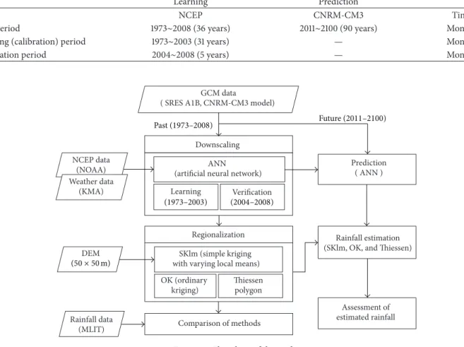
This study suggests a methodology that can account for geomorphologic characteristics when applying downscaling and regionalization techniques as a way to estimate rainfall in a basin by using GCM data. To this end, this study adopts CNRM-CM3 GCM model and SRES A1B for 1973– 2100. ANN is built for downscaling of the GCM data by applying learning and verification using monthly data, NCEP data of the NOAA, and weather data of the KMA (of a 36-year period). SKlm is applied for regionalization of the downscaled GCM using a Digital Elevation Model (DEM) and is compared with ordinary kriging (OK) and Thiessen methods in 26 rainfall stations of MLIT. The techniques will be used to predict and assess the monthly rainfall by future GCM data. The study procedure is shown inFigure 3.

3.1. ANN Model. In order to construct the ANN model by

spatial downscaling of GCM weather data, this study set the average temperature, specific humidity, wind speed, and average atmospheric pressure at sea level as the input layer and the monthly rainfall as the output layer. As seen in Figure 4, a multilayered ANN model consisting of one input layer, two hidden layers, and one output layer has been built. Monthly NCEP data from 1973 to 2008 (36 years) had been used for the learning period. For the forecast period, data from 2011 to 2100 (90 years) had been used based on CNRM-CM3 weather data (Table 1). Five years from the learning period (2004 to 2008) were set up as examination periods and the applicability of the constructed ANN model was reviewed by comparing it to observed data.

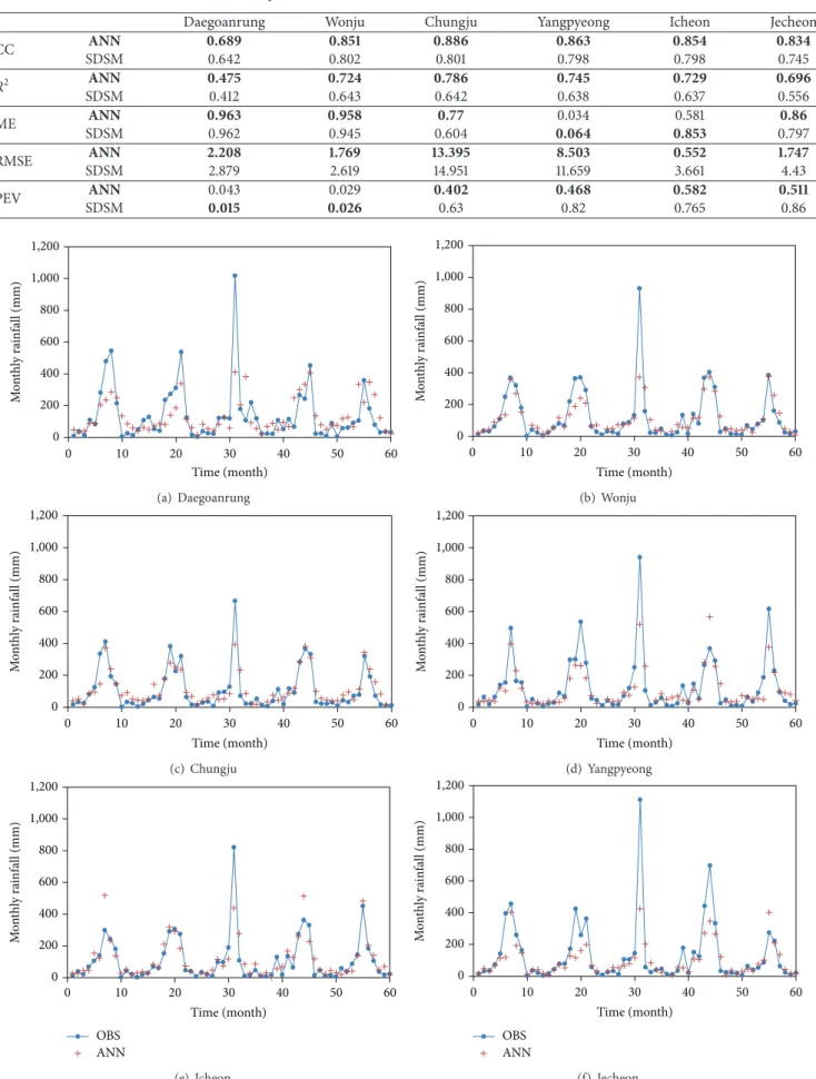
The output results of the 60-month (five-year) period for six weather stations were examined in the Namhan river basin. The result was that though they could not reproduce the extreme values of observed monthly rainfall, they simu-lated the observed values fairly well. The verification of the ANN model for rainfall series is shown inFigure 5.

In order to examine the applicability of the ANN model constructed in this study, a comparison with the results of the statistical downscaling model (SDSM) [52] was done. SDSM can be considered a general statistical downscaling technique based on multiple regression analysis. According to the model validation measures, such as the coefficient of correlation (CC), coefficient of determination (R2), model efficiency (ME), root mean squared error (RMSE), and prediction error variance (PEV), ANN was better overall. The better results are shown in bold inTable 2.

3.2. SKlm. SKlm is a technique that can utilize secondary data

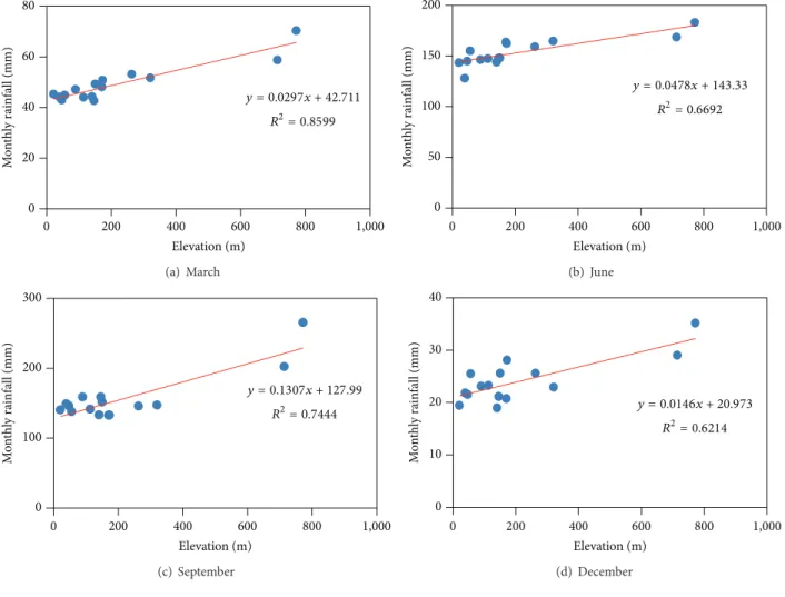
when performing spatial interpolation. This study used the Digital Elevation Model (DEM) as the secondary data for the spatial interpolation required for the downscaling technique. The relationship between elevation and monthly rainfall was analyzed for each month using the monthly averages of fifteen weather stations in the Namhan river basin.Figure 6 depicts the regression analysis results for March, June, September, and December. It was discovered that the eleva-tion and monthly rainfall have strong correlaeleva-tion with R2

(5)

Table 1: Input data of ANN.

Learning Prediction

Data NCEP CNRM-CM3 Time scale

Data period 1973∼2008 (36 years) 2011∼2100 (90 years) Monthly data

Learning (calibration) period 1973∼2003 (31 years) — Monthly data

Verification period 2004∼2008 (5 years) — Monthly data

GCM data

( SRES A1B, CNRM-CM3 model)

Downscaling Learning Thiessen polygon NCEP data (NOAA) Weather data (KMA) DEM Rainfall estimation (SKlm, OK, and Thiessen)

Assessment of estimated rainfall

Prediction ( ANN ) ANN

(artificial neural network) Verification

Regionalization SKlm (simple kriging with varying local means) OK (ordinary

kriging)

Rainfall data

(MLIT) Comparison of methods

Past (1973–2008)

(50 × 50 m)

(1973–2003) (2004–2008)

Future (2011–2100)

Figure 3: Flowchart of the study.

Specific humidity Mean temperature Sea level pressure Wind speed Monthly rainfall

Input layer Hidden layer Output layer

FHL-₁ FHL-2 SHL-₁ SHL-2 FHL-₈ FHL-₉ SHL-₈ SHL-₉ . . . . . .

Figure 4: Construction of ANN model.

between 0.62 and 0.86. The residuals of rainfall in each weather station were calculated using this primary regression relationship, and the SKlm technique was applied.

In order to examine the applicability of the SKlm tech-nique on 26 weather stations, this study applied and com-pared the Thiessen method and ordinary kriging (OK) method, which are general techniques in spatial interpola-tion.

The results of each method created by using fifteen weather stations are shown inFigure 7. Here the result of the Thiessen polygon method was expressed as fifteen values rep-resenting fifteen stations. The result of OK was expressed as spatial-interpolated values by the distances of fifteen stations. The result of SKlm was expressed as spatial-interpolated values by DEM and the distances of fifteen stations.

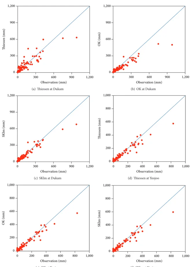
The spatial-interpolated data on two chosen weather stations with different elevations (Dukam (EL. 720 m) and Yeoju (EL. 45 m)) by applying Thiessen, OK, and SKlm techniques in sequence were compared with observed data and suggested in Figure 8. The rainfall of Dukam station, which is located at a high elevation, was estimated differently by each method. However the rainfall of Yeojoo station, which is located at a low elevation, was estimated similarly by each method.

According to the results of spatial interpolation from

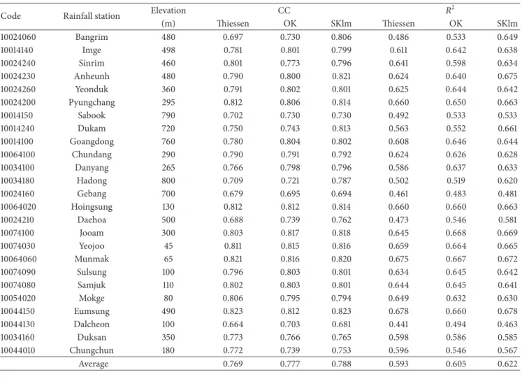
Figure 9andTable 3, it was found that the SKlm technique

reflects the geomorphologic characteristics (elevation) fairly well. CC and R2 on the forecasted values and observed

(6)

Table 2: Comparison of CC,𝑅2, ME, RMSE, and PEV of ANN and SDSM.

Daegoanrung Wonju Chungju Yangpyeong Icheon Jecheon

CC ANN 0.689 0.851 0.886 0.863 0.854 0.834 SDSM 0.642 0.802 0.801 0.798 0.798 0.745 𝑅2 ANN 0.475 0.724 0.786 0.745 0.729 0.696 SDSM 0.412 0.643 0.642 0.638 0.637 0.556 ME ANN 0.963 0.958 0.77 0.034 0.581 0.86 SDSM 0.962 0.945 0.604 0.064 0.853 0.797 RMSE ANN 2.208 1.769 13.395 8.503 0.552 1.747 SDSM 2.879 2.619 14.951 11.659 3.661 4.43 PEV ANN 0.043 0.029 0.402 0.468 0.582 0.511 SDSM 0.015 0.026 0.63 0.82 0.765 0.86 0 200 400 600 800 1,000 1,200 0 10 20 30 40 50 60 Time (month) M o n thl y ra infall (mm) (a) Daegoanrung 0 200 400 600 800 1,000 1,200 0 10 20 30 40 50 60 Time (month) M o n thl y ra infall (mm) (b) Wonju 0 200 400 600 800 1,000 1,200 0 10 20 30 40 50 60 Time (month) M o n thl y ra infall (mm) (c) Chungju 0 200 400 600 800 1,000 1,200 0 10 20 30 40 50 60 Time (month) M o n thl y ra infall (mm) (d) Yangpyeong 0 200 400 600 800 1,000 1,200 0 10 20 30 40 50 60 Time (month) M o n thl y ra infall (mm) OBS ANN (e) Icheon 0 200 400 600 800 1,000 1,200 0 10 20 30 40 50 60 Time (month) M o n thl y ra infall (mm) OBS ANN (f) Jecheon

(7)

0 20 40 60 80 0 200 400 600 800 1,000 M o n thl y ra infall (mm) Elevation (m) y = 0.0297x + 42.711 R2= 0.8599 (a) March 0 50 100 150 200 0 200 400 600 800 1,000 M o n thl y ra infall (mm) Elevation (m) y = 0.0478x + 143.33 R2_{= 0.6692} (b) June 0 100 200 300 0 200 400 600 800 1,000 M o n thl y ra infall (mm) Elevation (m) y = 0.1307x + 127.99 R2_{= 0.7444} (c) September 0 10 20 30 40 0 200 400 600 800 1,000 M o n thl y ra infall (mm) Elevation (m) y = 0.0146x + 20.973 R2= 0.6214 (d) December

Figure 6: Relation between elevation and monthly rainfall.

0–50 51–71 71–9191–110 111–130131–150 (a) Thiessen 140 80 60 20 (b) OK 140 80 60 20 (c) SKlm

Figure 7: Spatial interpolation results by each technique (unit: mm).

values on each technique were calculated for quantitative analysis. Consequently, it was found that the SKlm technique has the best applicability, with CC = 0.788 and R2 = 0.622. Characteristics of techniques had been reviewed and it has been found that the SKlm technique had the best result, when

weather stations are located at a high elevation. However, when weather station elevation was low, there was no large deviation among weather stations. The Thiessen and OK techniques were judged as having poor applicability because they could not consider the elevation factor.

(8)

0 300 600 900 1,200 0 300 600 900 1,200 Thies se n (mm) Observation (mm)

(a) Thiessen at Dukam

0 300 600 900 1,200 0 300 600 900 1,200 O K (mm) Observation (mm) (b) OK at Dukam 0 300 600 900 1,200 0 300 600 900 1,200 SK lm (mm) Observation (mm) (c) SKlm at Dukam 0 200 400 600 800 1,000 0 200 400 600 800 1,000 Thies se n (mm) Observation (mm) (d) Thiessen at Yeojoo 0 200 400 600 800 1,000 0 200 400 600 800 1,000 Observation (mm) O K (mm) (e) OK at Yeojoo 0 200 400 600 800 1,000 0 200 400 600 800 1,000 Observation (mm) SK lm (mm) (f) SKlm at Yeojoo

(9)

Table 3: Comparison of spatial interpolation techniques.

Code Rainfall station Elevation CC 𝑅

2 (m) Thiessen OK SKlm Thiessen OK SKlm 10024060 Bangrim 480 0.697 0.730 0.806 0.486 0.533 0.649 10014140 Imge 498 0.781 0.801 0.799 0.611 0.642 0.638 10024240 Sinrim 460 0.801 0.773 0.796 0.641 0.598 0.634 10024230 Anheunh 480 0.790 0.800 0.821 0.624 0.640 0.675 10024260 Yeonduk 360 0.791 0.802 0.801 0.625 0.644 0.642 10024200 Pyungchang 295 0.812 0.806 0.814 0.660 0.650 0.663 10014150 Sabook 790 0.702 0.730 0.730 0.492 0.533 0.533 10014240 Dukam 720 0.750 0.743 0.813 0.563 0.552 0.661 10014100 Goangdong 760 0.780 0.804 0.802 0.608 0.646 0.644 10064100 Chundang 290 0.790 0.791 0.792 0.624 0.626 0.628 10034100 Danyang 265 0.766 0.798 0.796 0.586 0.637 0.633 10034180 Hadong 800 0.709 0.721 0.787 0.502 0.519 0.620 10024160 Gebang 700 0.679 0.695 0.694 0.461 0.483 0.481 10064020 Hoingsung 130 0.812 0.812 0.814 0.660 0.660 0.663 10024210 Daehoa 500 0.688 0.739 0.762 0.473 0.546 0.581 10074100 Jooam 300 0.803 0.817 0.818 0.645 0.668 0.669 10074030 Yeojoo 45 0.811 0.815 0.816 0.659 0.664 0.665 10064060 Munmak 65 0.821 0.816 0.820 0.675 0.667 0.672 10074090 Sulsung 100 0.796 0.803 0.801 0.634 0.645 0.642 10074080 Samjuk 110 0.802 0.803 0.801 0.644 0.645 0.641 10054020 Mokge 80 0.806 0.795 0.794 0.649 0.632 0.630 10044150 Eumsung 490 0.823 0.812 0.823 0.678 0.660 0.678 10044130 Dalcheon 100 0.664 0.703 0.681 0.441 0.494 0.463 10034160 Duksan 350 0.773 0.766 0.765 0.598 0.586 0.585 10044010 Chungchun 180 0.772 0.739 0.753 0.596 0.546 0.567 Average 0.769 0.777 0.788 0.593 0.605 0.622 0.4 0.5 0.6 0.7 0.8 0 100 200 300 400 500 600 700 800 Thiessen OK SKlm C o efficien t o f det er mina tio n Elevation (m)

Trend (thiessen) Trend (OK) Trend (SKlm)

Figure 9: Trend of R2dependent on elevation.

When these characteristics were considered, it was judged that the SKlm technique will have better applicability in the Korean peninsula, which has relatively smaller density in the number of weather stations in the area with high elevation. In addition, it is expected that the SKlm technique will be quite useful as a downscaling technique, as it considers the geomorphologic characteristics of the Korean peninsula.

1,072 1,231 1,230 y = 2.7509x − 4478 Year Ann u al ra infall (mm) 1,800 1,600 1,400 1,200 1,000 800 600 2010 2020 2030 2040 2050 2060 2070 2080 2090 2100 Trend Estimated rainfall

Figure 10: Forecast of future annual rainfall levels using climate change scenario data.

3.3. Forecast of Future Monthly Rainfall under Climate Change.

In order to use the climate change scenario data in the scale of a basin, this study applied spatial downscaling techniques combining the ANN and SKlm techniques, which are believed to have better applicability, to the Namhan river

(10)

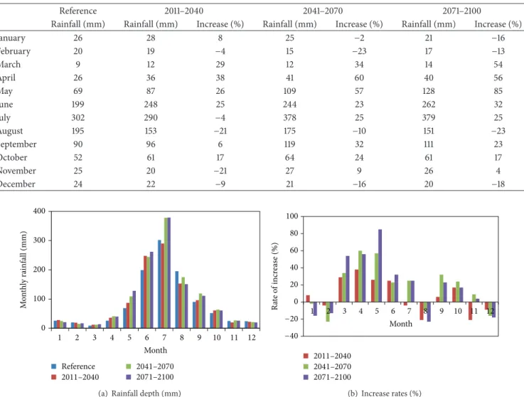
Table 4: Change of monthly rainfall in each target period.

Reference 2011–2040 2041–2070 2071–2100

Rainfall (mm) Rainfall (mm) Increase (%) Rainfall (mm) Increase (%) Rainfall (mm) Increase (%)

January 26 28 8 25 −2 21 −16 February 20 19 −4 15 −23 17 −13 March 9 12 29 12 34 14 54 April 26 36 38 41 60 40 56 May 69 87 26 109 57 128 85 June 199 248 25 244 23 262 32 July 302 290 −4 378 25 379 25 August 195 153 −21 175 −10 151 −23 September 90 96 6 119 32 111 23 October 52 61 17 64 24 61 17 November 25 20 −21 27 9 26 4 December 24 22 −9 21 −16 20 −18 0 100 200 300 400 1 2 3 4 5 6 7 8 9 10 11 12 M o n thl y ra infall (mm) Month Reference 2011–2040 2041–20702071–2100

(a) Rainfall depth (mm)

0 20 40 60 80 100 1 2 3 4 5 6 7 8 9 10 11 12 R at e o f incr ea se (%) Month 2011–2040 2041–2070 2071–2100 −20 −40 (b) Increase rates (%)

Figure 11: Change of monthly rainfall in each target period.

basin. The monthly average rainfall of the Namhan river basin until the year 2100 had been forecasted by getting the average of results downscaled to the spatial resolution of 50× 50 m. The change of annual average rainfall levels, which had been prepared based on the aforementioned results, is in Figure 10. According to the results of a primary regression, the annual rainfall is in an increasing trend. When the averages of forecasted rainfalls were calculated by segmenting those to 30-year target periods each, the result suggested that the rainfall after the later part of the 21st century will show a converging trend. It is believed that this result reflects the characteristics of the A1B climate change scenario, which reflects human effort to reduce carbon gas emission.

In order to examine the impact of climate change on the Namhan river basin in more detail, the changes in the characteristics of monthly runoffs from 2011 to 2100 were divided into three target periods (reference period, 2011– 2040, 2041–2070, and 2071–2100). The analysis results fore-casted that rainfall will increase during the rainy season (June and July) and decrease in the dry season (December, January, and February) inFigure 11andTable 4. The results

also suggested that the big increase of rainfall during the rainy season will cause the future annual rainfall to increase (Figure 11(a)). According to the analysis results of monthly increasing ratios, the rainfall increasing ratios in spring (March, April, and May) will be bigger (Figure 11(b)). The reason for this is believed to be the earlier arrival of the rainy season relative to years past. In other words, the change in the temporal aspect will be an important factor along with the increase in the quantitative aspect.

4. Discussions

When GCM data was used for the impact evaluation of climate change, the downscaling technique was typically applied. However, existing downscaling techniques have lim-itations in reproducing the rainfall characteristics that have large spatial variability in mountainous areas. As a methodol-ogy to address this issue, the ANN and SKlm techniques, both of which can use secondary data when performing spatial interpolation, were applied together and the results were compared to the Thiessen and ordinary kriging techniques,

(11)

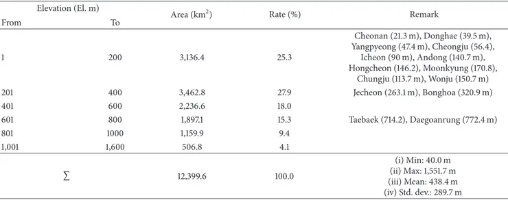
Table 5: Geomorphologic characteristics of the Namhan river basin. Elevation (El. m)

Area (km2) Rate (%) Remark

From To 1 200 3,136.4 25.3 Cheonan (21.3 m), Donghae (39.5 m), Yangpyeong (47.4 m), Cheongju (56.4), Icheon (90 m), Andong (140.7 m), Hongcheon (146.2), Moonkyung (170.8), Chungju (113.7 m), Wonju (150.7 m) 201 400 3,462.8 27.9 Jecheon (263.1 m), Bonghoa (320.9 m) 401 600 2,236.6 18.0 601 800 1,897.1 15.3 Taebaek (714.2), Daegoanrung (772.4 m) 801 1000 1,159.9 9.4 1,001 1,600 506.8 4.1 ∑ 12,399.6 100.0 (i) Min: 40.0 m (ii) Max: 1,551.7 m (iii) Mean: 438.4 m (iv) Std. dev.: 289.7 m

which are general downscaling techniques. According to the results (Figure 8andTable 3), the SKlm technique using the elevation data (DEM data) in the basin performed better than existing techniques. The reason for this is that rainfall deviations at different elevations have a significant impact on the results, and the Namhan river basin is located in a mountainous area. The elevations of the Namhan river basin were at minimum elevation of 40 m and at maximum elevation of 1551.7 m, where the difference is more than 1,000 m (Table 5). The average elevation is 438.4 m and the standard deviation is 289.7 m, which means that the elevation deviations are significantly large. Therefore, the estimated values could have poor accuracy if existing planar spatial interpolation techniques are applied. In general, it is known that elevation and rainfall have a strong positive correlation. Most of the weather stations in the Namhan river basin are located in a low elevation area (less than elevation of 300 m), excluding the Daegwanryeong weather station, which is at an elevation of 772.4 m. The weather stations are located in such a low elevation area because the station management and maintenance convenience were put on a higher priority than obtaining accurate data. Since most of the Korean peninsula is mountainous, it was judged that this issue was causing an underestimation of rainfall levels.

Based on the above results, the Thiessen, OK, and SKlm techniques were combined in the forecasting and comparison of future aerial average rainfalls of the Namhan river basin (Table 6). Consequently, the SKlm technique produced the biggest average rainfall for the Namhan river basin and the Thiessen technique produced the smallest average rainfall. The difference between the SKlm technique and the Thiessen technique was 70 mm during the reference period and 91 mm for the period of 2071 to 2100. In other words, it was observed that the deviation gets bigger as the time frame progresses into the future.

Based on the results ofSection 3.2, if the SKlm technique was the best technique in representing the rainfall spatial distribution characteristics of the Namhan river basin, it can

Table 6: Average rainfall from each spatial interpolation technique in the basin (mm). Thiessen (A) OK (B) SKlm (C) (C)−(A) (C)−(B) Reference 959 974 1,029 70 55 2011–2040 994 1,015 1,072 78 57 2041–2070 1,144 1,153 1,231 87 78 2071–2100 1,139 1,146 1,230 91 84

be said that the existing spatial interpolation techniques for climate change impact evaluation were seriously underfore-casting rainfall. Given the rapid increase of rainfall in the future rainy season as seen in the monthly analysis results (Figure 10, Table 3), if the plans to respond and adapt to climate change are established on the basis of the results produced by existing techniques, there will likely be many issues during the flood seasons in the future.

It can be said that rainfall in a basin may be affected by various complex elements such as meteorological characteris-tics, geomorphologic characterischaracteris-tics, and land coverage char-acteristics. This is especially the case for the Korean penin-sula, where rainfall events under the impact of the monsoon are usually dominant; however, extreme weather phenomena are heavily impacted by tropical cyclones, such as typhoons. It is also true that there are large deviations between regions due to the geomorphologic characteristics of a mountainous area. These issues are causing many difficulties in the accurate estimation of rainfall in basins when evaluating the impact of climate change.

This study focused on the influence of geomorphologic characteristics of a basin in order to produce more accurate rainfall data using future weather data from GCMs. Among these geomorphologic characteristics, the impact of elevation data was examined as a factor and was found to have the biggest impact on rainfall variability. However, it was believed

(12)

that examination on the slope and aspect of basin, which had been made by river flow, was also required for considering the characteristics of the Korean peninsula, which is affected by the monsoon and tropical cyclones. The accuracy of aerial rainfall estimation in the basin would be effectively enhanced if these impacts are comprehensively reflected.

5. Conclusions

By themselves, general downscaling techniques that down-scale GCM data to a location in a basin cannot properly reproduce the weather characteristics of the region, especially in a mountainous area. In order to address this issue, this study suggested a downscaling and regionalization technique, which is needed for the climate change impact evaluation using GCM data in a basin or region, and examined the changes in the future rainfall characteristics. A methodology which applied the technique considering the basin geomor-phologic characteristics and which combined the ANN and SKlm techniques was suggested. It was found that the SKlm technique had better applicability in mountainous areas like the Korean peninsula than the existing techniques such as the Thiessen polygon method or ordinary kriging.

The methodology suggested in this study was applied on the CNRM-CM3 model results, which was a simulation of the SRES A1B scenario. The future monthly average rainfall was forecasted for the Namhan river basin. According to the forecasted results of the monthly average rainfall in the basin, the total rainfall will continuously increase in the future. There were also notable trends, such as the increasing rainfall trend during the rainy season and the decreasing rainfall trend during the dry season. Furthermore, it was discovered that the arrival of the rainy season will shift to an earlier point in time.

By comparing the results generated by our novel approach against the future annual average rainfall forecasted by exist-ing methodologies, we found that there were substantially large deviations that were dependent on the techniques used. It was discovered that the choice of methodology was a significant factor in the success or failure of future water resources planning. Therefore, the methodology suggested by this study, which was found to have good applicability to mountainous areas, could contribute to the establishment of successful water resources planning in the future. It may also provide some information that helps us overcome the limitations that statistical downscaling techniques suffer in low spatial resolutions when compared to their dynamical downscaling counterparts.

Conflict of Interests

The authors declare that there is no conflict of interests regarding the publication of this paper.

Acknowledgments

This work was supported by the National Research Founda-tion of Korea (NRF) and by a Grant funded by the Korean Government (MEST) (no. 2011-0028564).

References

[1] T. G. Huntington, “Evidence for intensification of the global water cycle: review and synthesis,” Journal of Hydrology, vol. 319, no. 1–4, pp. 83–95, 2006.

[2] IPCC, The First Assessment Report (FAR), Cambridge University Press, Cambridge, UK, 1990.

[3] IPCC, The Second Assessment Report: Climate Change 1995

(SAR), Cambridge University Press, Cambridge, UK, 1995.

[4] IPCC, The Third Assessment Report: Climate Change 2001 (TAR), Cambridge University Press, New York, NY, USA, 2001. [5] IPCC, The Fourth Assessment Report: Climate Change 2007

(AR4), Cambridge University Press, New York, NY, USA, 2007.

[6] IPCC, The Fifth Assessment Report : Climate Change 2013(AR5), Cambridge University Press, Great Britain, Cambridge, UK, 2013.

[7] F. Giorgi, B. Hewitson, J. Christensen et al., “Regional climate information—evaluation and projections,” in Climate Change

2001: The Scientific Basis, J. T. Houghton, Y. Ding, D. J. Griggs et

al., Eds., p. 944, Cambridge University Press, Cambridge, UK, 2001.

[8] L. O. Mearns, F. Giorgi, P. Whetton, D. Pabon, M. Hulme, and M. Lal, “Guidelines for use of climate scenarios developed from regional climate model experiments,” Tech. Rep., Data Distribution Centre of the Intergovernmental Panel on Climate Change, Norwich, UK, 2003.

[9] E. P. Maurer, A. W. Wood, J. C. Adam, D. P. Lettenmaier, and B. Nijssen, “A long-term hydrologically based dataset of land surface fluxes and states for the conterminous United States,”

The Americam Meteorological Society, vol. 15, no. 22, pp. 3237–

3251, 2002.

[10] H. J. Fowler, S. Blenkinsop, and C. Tebaldi, “Linking climate change modelling to impacts studies: recent advances in down-scaling techniques for hydrological modelling,” International

Journal of Climatology, vol. 27, no. 12, pp. 1547–1578, 2007.

[11] C. Frei, R. Sch¨oll, S. Fukutome, J. Schmidli, and P. L. Vidale, “Future change of precipitation extremes in Europe: Intercom-parison of scenarios from regional climate models,” Journal of

Geophysical Research, vol. 111, no. D6, Article ID D06105, 2006.

[12] J. W. Hurrell, G. J. Holland, and W. G. Large, “The nested regional climate model: an approach toward prediction across scales,” in Proceedings of the AGU Fall Meeting, vol. 89, Eos, Transactions American Geophysical Union, 2008.

[13] L. O. Mearns, W. Gutowski, R. Jones et al., “A regional climate change assessment program for North America,” Eos,

Transac-tions American Geophysical Union, vol. 90, no. 36, p. 311, 2009.

[14] M. Hulme, G. J. Jenkins, X. Lu et al., Climate Change Scenarios

for the United Kingdom: The UKCIP02 Scientific Report, Tyndall

Centre for Climate Change Research, University of East Anglia, Norwich, UK, 2002.

[15] J. H. Christensen, T. R. Carter, M. Rummukainen, and G. Amanatidis, “Evaluating the performance and utility of regional climate models: the PRUDENCE project,” Climatic Change, vol. 81, no. 1, pp. 1–6, 2007.

[16] X. Gao, J. S. Pal, and F. Giorgi, “Projected changes in mean and extreme precipitation over the Mediterranean region from a high resolution double nested RCM simulation,” Geophysical

Research Letters, vol. 33, no. 3, Article ID L03706, 2006.

[17] F. Giorgi, X. Bi, and J. S. Pal, “Mean, interannual variability and trends in a regional climate change experiment over Europe. I. Present-day climate (1961–1990),” Climate Dynamics, vol. 22, no. 6-7, pp. 733–756, 2004.

(13)

[18] J. Marengo and T. Ambrizzi, “Use of regional climate models in impact assessments and adaptations studies from continental to regional and local scales: The CREAS (Regional Climate Change Scenarios for South America) initiative in South America,” in

Proccedings of the 8th International Conference on Southern Hemisphere Meteorology and Oceanography (ICSHMO ’06), pp.

291–296, 2006.

[19] R. L. Wilby, S. P. Charles, E. Zorita, B. Timbal, P. Whetton, and L. O. Mearns, “Guidelines for the use of climate scenarios devel-oped from statistical downscaling methods,” Tech. Rep., IPCC Task Group on Data and Scenario Support for Impact and Climate Analysis (TGICA), Norwich, UK, 2004.

[20] C. M. Goodess, C. Anagnostopoulo, A. Bardossy et al., “An intercomparison of statistical downscaling methods for Europe and European regions—assessing their performance with respect to extreme temperature and precipitation events,” Tech. Rep. CRU RP11, University of East Anglia, Climate Research Unit Research Publications, Norfolk, UK, 2012.

[21] I. Hanssen-Bauer and E. J. Førland, “Long-term trends in pre-cipitation and temperature in the Norwegian Arctic: can they be explained by changes in atmospheric circulation patterns?”

Climate Research, vol. 10, no. 2, pp. 143–153, 1998.

[22] C. Hellström, D. Chen, C. Achberger, and J. Räisänen, “Compar-ison of climate change scenarios for Sweden based on statistical and dynamical downscaling of monthly precipitation,” Climate

Research, vol. 19, no. 1, pp. 45–55, 2001.

[23] U. Cubasch, H. von Storch, J. Waszkewitz, and E. Zorita, “Estimates of climate change in southern Europe derived from dynamical climate model output,” Climate Research, vol. 7, no. 2, pp. 129–149, 1996.

[24] J. W. Kidson and C. S. Thompson, “A comparison of statistical and model-based downscaling techniques for estimating local climate variations,” Journal of Climate, vol. 11, no. 4, pp. 735–753, 1998.

[25] I. Hanssen-Bauer, E. J. Førland, J. E. Haugen, and O. E. Tveito, “Temperature and precipitation scenarios for Norway: com-parison of results from dynamical and empirical downscaling,”

Climate Research, vol. 25, no. 1, pp. 15–27, 2003.

[26] J.-L. Chu, H. Kang, C.-Y. Tam, C.-K. Park, and C.-T. Chen, “Seasonal forecast for local precipitation over northern Taiwan using statistical downscaling,” Journal of Geophysical Research, vol. 113, no. 12, Article ID D12118, 2008.

[27] E. Zorita and H. von Storch, “The analog method as a simple statistical downscaling technique: comparison with more com-plicated methods,” Journal of Climate, vol. 12, no. 8, pp. 2474– 2489, 1999.

[28] Yuval and W. W. Hsieh, “An adaptive nonlinear scheme for pre-cipitation forecasts using neural networks,” Weather and

Fore-casting, vol. 18, no. 2, pp. 303–310, 2003.

[29] Y. B. Dibike and P. Coulibaly, “Temporal neural networks for downscaling climate variability and extremes,” Neural

Net-works, vol. 19, no. 2, pp. 135–144, 2006.

[30] A. Pasini and R. Langone, “Attribution of precipitation changes on a regional scale by neural network modeling: a case study,”

Water, vol. 2, no. 3, pp. 321–332, 2010.

[31] T. R. Karl, W. C. Wang, M. E. Schlesinger, R. W. Knight, and D. Portman, “A method of relating general circulation model simulated climate to the observed local climate. Part I: seasonal statistics,” Journal of Climate, vol. 3, no. 10, pp. 1053–1079, 1990. [32] T. M. L. Wigley, P. D. Jones, K. R. Briffa, and G. Smith, “Obtain-ing sub-grid-scale information from coarse-resolution general

circulation model output,” Journal of Geophysical Research, vol. 95, no. 2, pp. 1943–1953, 1990.

[33] H. Von Storch, E. Zorita, and U. Cubasch, “Downscaling of global climate change estimates to regional scales: an applica-tion to Iberian rainfall in wintertime,” Journal of Climate, vol. 6, no. 6, pp. 1161–1171, 1993.

[34] A. Busuioc, D. Chen, and C. Hellstr¨om, “Temporal and spatial variability of precipitation in Sweden and its link with the large-scale atmospheric circulation,” Tellus, vol. 53, no. 3, pp. 348–367, 2001.

[35] R. Huth, “Statistical downscaling of daily temperature in central Europe,” Journal of Climate, vol. 15, no. 13, pp. 1731–1742, 2002. [36] R. Tomozeiu, C. Cacciamani, V. Pavan, A. Morgillo, and A.

Busuioc, “Climate change scenarios of surface temperature in Emilia-Romagna (Italy) obtained using statistical downscaling,”

Theoretical and Applied Climatology, vol. 90, no. 1-2, pp. 25–47,

2006.

[37] M. D. Fr´ıas, E. Zorita, J. Fern´andez, and C. Rodr´ıguez-Puebla, “Testing statistical downscaling methods in simulated climates,”

Geophysical Research Letters, vol. 33, no. 19, Article ID L19807,

2006.

[38] M. S. Kyoung, H. S. Kim, B. Sivakumar, V. P. Singh, and K. S. Ahn, “Dynamic characteristics of monthly rainfall in the Korean Peninsula under climate change,” Stochastic

Environ-mental Research and Risk Assessment, vol. 25, no. 4, pp. 613–625,

2011.

[39] L. E. Hay and M. P. Clark, “Use of statistically and dynamically downscaled atmospheric model output for hydrologic simula-tions in three mountainous basins in the western United States,”

Journal of Hydrology, vol. 282, no. 1–4, pp. 56–75, 2003.

[40] J. Schmidli, C. M. Goodess, C. Frei et al., “Statistical and dynam-ical downscaling of precipitation: an evaluation and comparison of scenarios for the European Alps,” Journal of Geophysical

Research, vol. 112, no. 4, Article ID D04105, 2007.

[41] S. Spak, T. Holloway, B. Lynn, and R. Goldberg, “A comparison of statistical and dynamical downscaling for surface temper-ature in North America,” Journal of Geophysical Research D:

Atmospheres, vol. 112, no. 8, Article ID D08101, 2007.

[42] E. D. Gutmann, R. M. Rasmussen, C. Liu et al., “A comparison of statistical and dynamical downscaling of winter precipitation over complex terrain,” Journal of Climate, vol. 25, no. 1, pp. 262– 281, 2012.

[43] S.-T. Chen, P.-S. Yu, and Y.-H. Tang, “Statistical downscaling of daily precipitation using support vector machines and multi-variate analysis,” Journal of Hydrology, vol. 385, no. 1–4, pp. 13– 22, 2010.

[44] M. Kyoung, Assessment of climate change effect on standardized

precipitation index and frequency-based precipitation [Doctoral dissertation], Inha University, Incheon, Korea, 2010.

[45] Y. A. Kwon, W. T. Kwon, K. O. Boo, and Y. E. Choi, “Future projections on subtropical climate regions over south korea using SRES A1B data,” The Korean Geographical Society, vol. 42, no. 3, pp. 355–367, 2007.

[46] R. J. Kuligowski and A. P. Barros, “Localized precipitation fore-casts from a numerical weather prediction model using artificial neural networks,” Weather and Forecasting, vol. 13, no. 4, pp. 1195–1205, 1998.

[47] C. M. Bishop, Neural Networks for Pattern Recognition, Claren-don Press, LonClaren-don, UK, 2000.

[48] P. Picton, Neural Networks, Palgrave, Basingstoke, UK, 2nd edi-tion, 2000.

(14)

[49] W. Hsieh, Machine Learning Methods in the Environmental

Sciences, Cambridge University Press, Cambridge, UK, 2009.

[50] S. Haupt, A. Pasini, and C. Marzban, Artificial Intelligence

Meth-ods in the Environmental Sciences, Springer, 2009.

[51] P. Goovaerts, Geostatistics for Natural Resources Evaluation, Oxford University Press, New York, NY, USA, 1997.

[52] R. L. Wilby, C. W. Dawson, and E. M. Barrow, “SDSM—a decision support tool for the assessment of regional climate change impacts,” Environmental Modelling and Software, vol. 17, no. 2, pp. 147–159, 2002.

(15)