HAL Id: hal-01382110
https://hal.archives-ouvertes.fr/hal-01382110
Submitted on 15 Oct 2016
HAL is a multi-disciplinary open access
archive for the deposit and dissemination of
sci-entific research documents, whether they are
pub-lished or not. The documents may come from
teaching and research institutions in France or
L’archive ouverte pluridisciplinaire HAL, est
destinée au dépôt et à la diffusion de documents
scientifiques de niveau recherche, publiés ou non,
émanant des établissements d’enseignement et de
recherche français ou étrangers, des laboratoires
limits
Philippe Carmona, Nicolas Pétrélis
To cite this version:
Philippe Carmona, Nicolas Pétrélis. Interacting partially directed self avoiding walk: scaling limits.
Electronic Journal of Probability, Institute of Mathematical Statistics (IMS), 2016, 21 (49), pp.1-52.
�10.1214/16-EJP4618�. �hal-01382110�
E l e c t ro n ic Jo f P r o b a b i l i t y Electron. J. Probab. 21 (2016), no. 49, 1–52. ISSN: 1083-6489 DOI: 10.1214/16-EJP4618
Interacting partially directed self avoiding walk:
scaling limits
Philippe Carmona
*Nicolas Pétrélis
*Abstract
This paper is dedicated to the investigation of a1 + 1dimensional self-interacting and partially directed self-avoiding walk. The intensity of the interaction between monomers is denoted by 2 (0, 1)and there exists a critical threshold cwhich
determines the three regimes displayed by the model, i.e., extended for < c,
critical for = cand collapsed for > c.
In [4], physicists displayed some numerical results concerning the typical growth rate of some geometric features of the path as its length L diverges. From this perspective the quantities of interest are the horizontal extension of the path and its lower and upper envelopes.
With the help of a new random walk representation, we proved in [10] that the path grows horizontally likepLin its collapsed regime and that, once rescaled by
p
Lvertically and horizontally, its upper and lower envelopes converge towards some deterministic Wulff shapes.
In the present paper, we bring the geometric investigation of the path several steps further. In the collapsed regime, we identify the joint limiting distribution of the fluctuations of the upper and lower envelopes around their associated limiting Wulff shapes, rescaled in time bypLand in space byL1/4. In the critical regime we
identify the limiting distribution of the horizontal extension rescaled byL2/3and we
show that the excess partition function decays asL2/3with an explicit prefactor. In
the extended regime, we prove a law of large number for the horizontal extension of the polymer rescaled by its total lengthL, we provide a precise asymptotics of the partition function and we show that its lower and upper envelopes, once rescaled in time byLand in space bypL, converge towards the same Brownian motion.
Keywords: Polymer collapse; phase transition; Brownian area; large deviations. AMS MSC 2010: Primary 60K35, Secondary 82B26; 82B41; 60F10.
Submitted to EJP on October 9, 2015, final version accepted on July 7, 2016.
*Laboratoire de Mathématiques Jean Leray UMR 6629, Université de Nantes, France.
E-mail: [email protected] E-mail: [email protected]
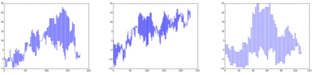
Figure 1: Simulations of IPDSAW for critical temperature = c and lengthL = 1600
1 Introduction
We consider a model of statistical mechanics introduced in [34] and referred to as interacting partially directed self avoiding walk (IPDSAW). The model is a (1 + 1)-dimensional partially directed version of the interacting self-avoiding walk (ISAW) introduced in [18] as a model for an homopolymer in a poor solvent.
The aim of our paper is to pursue the investigation of the IPDSAW initiated in [29] and [10] and in particular to display the infinite volume limit of some features of the model when the size of the system diverges for each of the three regimes: collapsed, critical and extended. The first object to be considered is the horizontal extension of the path. Then, we will consider the whole path, properly rescaled and look at its infinite volume limit in the extended phase and in the collapsed phase.
Let us point that numerical simulations are difficult (see e.g. [4]) and have not led to theoretical results about the path properties of the polymer in the three regimes that we establish in this paper.
1.1 Model
The model can be defined in a simple manner. An allowed configuration for the polymer is given by a family of oriented vertical stretches. To be more specific, for a polymer made of L 2 N monomers, the possible configurations are gathered in
⌦L :=SLN =1LN,L, where LN,Lis the set consisting of all families made of N vertical stretches that have a total lengthL N, that is
LN,L= n l2 ZN :PN n=1|ln| + N = L o . (1.1)
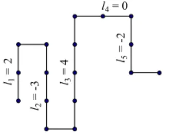
Note that with such configurations, the modulus of a given stretch corresponds to the number of monomers constituting this stretch (and the sign gives the direction upwards or downwards). Moreover, any two consecutive vertical stretches are separated by a monomer placed horizontally and this explains whyPNn=1|ln|must equalL Nin order forl = (li)Ni=1 to be associated with a polymer made ofLmonomers (see Fig. 2).
The repulsion between the monomers and the solvent around them is taken into account in the Hamiltonian associated with each pathl2 ⌦Lby rewarding energetically those pairs of consecutive stretches with opposite directions, i.e.,
HL, (l1, . . . , lN) = Pn=1N 1(ln^ le n+1), (1.2) where x^ y =e ( |x| ^ |y| ifxy < 0, 0 otherwise. (1.3)
One can already note that large Hamiltonians will be assigned to trajectories made of few but long vertical stretches with alternating signs. Such paths will be referred to
l1 = 2 l2 = -3 l =3 4 l =5 -2 l4 = 0
Figure 2: Example of a trajectoryl2 LN,LwithN = 5vertical stretches, a total length L = 16and an HamiltonianHL, (⇡) = 5 .
as collapsed configurations. With the Hamiltonian in hand we can define the polymer measure as
PL, (l) = e HL, (l)
ZL,
, l2 ⌦L, (1.4)
whereZL, is the partition function of the model, i.e., ZL, = L X N =1 X l2LN,L eHL, (l). (1.5)
1.2 Random walk representation and collapse transition
An alternative probabilistic representation of the partition function has been intro-duced in [29]. For > 0we introduce an auxiliary random walkV = (Vi)1i=0of lawP , starting from0, and whose increments(Ui)1i=0 are i.i.d. and follow a discrete Laplace distribution, i.e., P (U1= k) = e 2 | k| c 8k 2 Z with c := 1+e /2 1 e /2. (1.6)
Such walk allows us to provide an alternative expression of the partition function, i.e.,
e ZL, = e LZL, = c L X N =1 ( )NP (V 2 VN,L N), (1.7)
where VN,L N := {V : GN(V ) = L N, VN +1 = 0}, whereGN(V ) := PNi=1|Vi| is the geometric area in betweenV and the horizontal axis up to timeN and where
= c
e and c :=
1 + e /2
1 e /2. (1.8)
For later use, we also introduceAN(V ) :=PNi=1Vithe algebraic counterpart ofGN(V ). We will recall briefly in Section 3.1 how (1.7) can be obtained, but let us observe already that the excess free energy defined as
e
f ( ) := lim L!1
1
Llog eZL, (1.9)
loses its analyticity at c, the unique solution of = 1. For c the inequality 1 indeed yields that f ( ) = 0e since those terms indexed by N ⇠ pL in (1.7) decay subexponentially. As a consequence the trajectories dominatingZeL, have a small horizontal extension, i.e.,N = o(L). When < cin turn, > 1and since forc2 (0, 1] the quantityP (VcL,(1 c)L)decays exponentially fast with a rate that vanishes asc! 0
we can claim that the dominating trajectories inZeL, have an horizontal extension of orderL, and moreover thatf ( ) > 0e . The phase diagram[0,1)is therefore partitioned into a collapsed phase denoted byCand an extended phase denoted byE, i.e,
C := { : ef ( ) = 0} = { : c}, (1.10)
E := { : ef ( ) > 0} = { : < c}.
We shall see that, in fact, there are three regimes; collapsed ( > c), critical ( = c) and extended ( < c), in which the asymptotics of the partition function and the path properties are radically different.
2 Main results
We observe that the definition of the polymer measure in (1.4) is left unchanged if we replace the denominator byZeL, (cf (1.7)) and substractL to the Hamiltonian.
2.1 Scaling limit of the horizontal extension
Displaying sharp asymptotic estimates of the partition function as the system size diverges is a major issue in statistical mechanics. Computing the probability mass of a certain subset of trajectories under the polymer measure indeed requires to have a good control on the denominator in (1.4). For the extended and the critical regimes, we display in Theorem 2.1 below an equivalent of the partition function allowing us e.g to exhibit the polynomial decay rate of the partition function at the critical point. For the collapsed regime, in turn, we recall the bounds onZeL, that had been obtained in [10] allowing us to identify its sub-exponential decay rate.
Note that in Remark 2.3 below, we provide some complements concerning Theo-rems 2.1 and 2.2 among which the exact value of some pre-factors when an expression is available. We also denote byfex the density of the area below a normalized Brow-nian excursion (see e.g. [25]) and we set C := (E (V2
1)) 1/2. Thus, we can define w(x) = C fex(C x). We recall the definition off ( )e in (1.9).
Theorem 2.1 (Asymptotics of the partition function). (1) For < c, there exists ac > 0 such that
e
ZL, = c ef ( )Le (1 + o(1)), (2) for = c, there exists ac > 0such that
e ZL, = c L2/3(1 + o(1)) with c = 1 + e 2 (24 ⇡ E (V2 1)) 1 2 R+1 0 x 3w(x 3 2) dx ,
(3) for > c, there exists a unique real numberm( ) > 0andc1, c2, > 0such that c1 Le m( )pL eZL, c2 p Le m( )pL for L 2 N.
For eachl2 ⌦L, the variableNldenotes the horizontal extension ofl, i.e., the integer N 2 {1, . . . , L}such thatl 2 LN,L. Theorem 2.2 below gives the scaling limit of the horizontal extension of a typical pathlsampled fromPL, and asL! 1(for the sake of completeness, we again integrate the collapsed regime into the theorem although this regime was dealt with in [10, Theorem D]).
Theorem 2.2 (Horizontal extension). (1) if < c, there exists a real constante( )2 (0, 1)such that lim L!1PL, ⇣ Nl L e( ) " ⌘ = 0. (2.1)
(2) if = c, then lim L!1 Nl L2/3 =lawC 2/3 g1, where ga = inf n t > 0R0t|Bs| ds = a o
is the continuous inverse of the geometric Brownian area, and we considerg1under the conditional law of the Brownian motion conditioned byBg1= 0.
(3) If > c, there exists a unique real numbera( ) > 0such that lim L!1PL, ⇣ Nl p L a( ) " ⌘ = 0. (2.2) Remark 2.3.
(1) For the extended regime, in Section 6, we will decompose each path into a succes-sion of patterns (sub pieces) and we will associate with our model an underlying regenerative process ( i, ⌫i, yi)i2N of lawP in such a way that i (resp. ⌫i, resp. yi) plays the role of the number of monomers constituting theith pattern (resp. the horizontal extension of theith pattern, resp. the vertical displacement of the ith pattern). Then, the constantcin Theorem 2.1 (1) and the limiting rescaled horizontal extension in Theorem 2.2 (1) satisfy
c = E (1 1) and e( ) = E (⌫1) E ( 1).
(2) For the critical regime = c, the appearance of the distribution ofg1is explained at the end of Section 4.
2.2 Scaling limit of the vertical extension
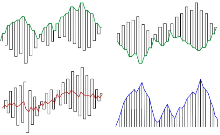
The fact that each trajectoryl 2 ⌦L is made of a succession of vertical stretches makes it convenient to give a representation of the trajectory in terms of its upper and lower envelopes. Thus, we pickl2 LN,Land we letEl+ = (E
+ l,i)
N +1
i=0 andEl = (El,i) N +1 i=0 be the upper and the lower envelopes ofl, i.e., the(1 + N )-step paths that link the top and the bottom of each stretch consecutively. Thus,E+
l,0=El,0= 0, E+
l,i= max{l1+· · · + li 1, l1+· · · + li}, i 2 {1, . . . , N}, (2.3) El,i= min{l1+· · · + li 1, l1+· · · + li}, i 2 {1, . . . , N}, (2.4) andE+
l,N +1=El,N +1= l1+· · · + lN (see Fig. 3). Note that the area in between these two envelopes is completely filled by the path and therefore, we will focus on the scaling limits ofE+
l andEl .
At this stage, we defineY : [0, 1]e ! Rto be the time-space rescaled cadlag process of a given(Yi)N +1i=0 2 ZN +1satisfyingY0= 0. Thus,
e
Y (t) = 1
N + 1Ybt (N+1)c, t2 [0, 1], (2.5)
and for eachl 2 LN,Lwe letEel+,Eel be the time-space rescaled processes associated with the upper envelopeE+
l and with the lower envelopeEl , respectively.
In this paper we will focus on the infinite volume limit of the whole path inside the collapsed phase ( > c) and in the extended phase ( < c). Concerning the critical regime ( = c) this limit will be discussed as an open problem in Section 2.3 below.
Figure 3: Example of the upper envelope left picture), of the lower envelope (top-right picture), of the middle line (bottom left picture) and of the profile (bottom (top-right picture) of a given trajectory (in dashed line).
The collapsed phase ( > c)
The collapsed regime was studied in [10], where a particular decomposition of the path into beads has been introduced. A bead is a succession of non-zero vertical stretches with alternating signs which ends when two consecutive stretches have the same sign (or when a stretch is null). Such a decomposition is meaningful geometrically and we proved in [10, Theorem C] that there is a unique macroscopic bead in the collapsed regime and that the number of monomers outside this bead are at most of order(log L)4.
The next step, in the geometric description of the path, consisted in determining the limiting shapes of the envelopes of this unique bead. This has been achieved in [10] where the rescaled upper envelope (respectively lower envelope) is shown to converge in probability towards a deterministic Wulff shape ⇤(resp. ⇤) defined as follows
⇤(s) =Z s 0 L0⇥(1 2 x)eh0( 1 a( )2, 0) ⇤ dx, s2 [0, 1], (2.6)
whereLis defined in (5.3) andeh0in (5.10). Thus, we obtained
Theorem 2.4. ([10] Theorem E) For > cand" > 0, lim L!1PL, ⇣ e El+ ⇤ 2 1> " ⌘ = 0, lim L!1PL, ⇣ e El + ⇤ 2 1> " ⌘ = 0. (2.7)
This Theorem has also been stated as a Shape Theorem in [10]. The natural question that comes to mind is: are we able to identify the fluctuations around this shape? For technical reasons that will be discussed in Remark 2.6 below, we are not able to identify such a limiting distribution. However, we can prove a close convergence result by working on a particular mixture of those measures PL0, for L0 2 KL := L+[ "(L), "(L)]\Nwith"(L) := (log L)6. Thus, we define the extended set of trajectories e
⌦L=[L02KL⌦L0, and we letPeL, be a mixture of those PL0, , L0 2 KL defined by e PL, l := X L02KL e ZL0, P k2KLZek, PL0, (l) 1{l2⌦L0}, forl2 e⌦L. (2.8)
In other words,PeL, satisfies e PL, · | ⌦L0 = PL0, (·) and PeL, ⌦L0 = e ZL0, P k2KLZek, , forL0 2 KL. (2.9) We denote byQeL, the law of the fluctuations of the envelopes around their limiting shapes, that is the law of the random processes
p Nl ⇣ e E+ l (s) ⇤(s) 2 , eEl (s) + ⇤(s) 2 ⌘ s2[0,1], (2.10)
withlsampled fromPeL, . Finally, let us note that stating Theorem 2.5 requires using functionHe that will be defined in Section 5.1. We obtain the following limit.
Theorem 2.5 (Fluctuations of the convex envelopes around the Wulff shape). For > c, andH = eH(q , 0), q = 1
a( )2 we have the convergence in distribution e QL, d ! L!1 ⇣ ⇠H+ ⇠c H 2 , ⇠H ⇠c H 2 ⌘ , (2.11)
where for H = (h0, h1)such that [h0, h0+ h1] ⇢ D = ( /2, /2), the process ⇠H = (⇠H(t), 0 t 1)is centered and Gaussian with covariance
E [⇠H(s) ⇠H(t)] = Z s^t
0
L00((1 x)h0+ h1) dx, and where⇠c
H:= (⇠Hc (t), 0 t 1)is a process independent of⇠H which has the law of ⇠H conditionally on⇠H(1) =R
1
0 ⇠H(s) ds = 0.
From Theorem 2.5 we deduce that the fluctuations of both envelopes around their limiting shapes are of orderL1/4.
Remark 2.6. The reason why we prove Theorem 2.5 under the mixture PeL, rather thanPL, is the following. We need to establish a local limit theorem for the associated random walk of lawP conditioned on having a large geometric areaGN(V )and we are unable to do it. Fortunately, we know how to condition the random walk on having a large algebraic areaAN(V )and under the mixturePeL, we are able to compare quantitatively these two conditionings (see Step 2 of the proof of Proposition 5.2 in Section 5.5).
In the construction of the mixture lawPeL, (cf. (2.8)), the choice of the prefactors of thosePL0, withL
0
2 KLmay appear artificial. However it is conjectured (see e.g. [20, Section 8]) that our inequalities in Theorem 2.1 (3) can be improved to
e
ZL, ⇠ B L3/4e
m( )pL withB > 0,
so that the ratio of any two prefactors would converges to1asL! 1uniformly on the choice of the indices of the two prefactors inKL. In other word,PeL, should, in first approximation, be the uniform mixture of those{PL0, , L02 KL}.
Remark 2.7. We observe that one can recover the envelopes from two auxiliary
pro-cesses, i.e, the middle lineMland the profile |l|. Thus, we associate with eachl2 LN,L the path|l| = (|li|)N +1i=0 (withlN +1= 0by convention) and the pathMl= Ml,i
N +1 i=0 that links the middles of each stretch consecutively, i.e.,Ml,0= 0and
Ml,i= l1+· · · + li 1+ li
2, i2 {1, . . . , N}, (2.12)
andMl,N +1 = l1+· · · + lN (see Fig. 3). With the help of (2.5), we letMflandelbe the time-space rescaled processes associated withMlandland one can easily check that
e
As a consequence, proving Theorem 2.5 is equivalent to proving that b QL, d ! L!1 ⇠H, ⇠ c H , (2.14)
whereQbL, is the law ofpNl Mfl(s),|el(s)| ⇤(s) s2[0,1]withlsampled fromPeL, . The convergence ofMflin (2.14) answers an open question raised in [4, Fig. 14 and Table II] where the process is referred to as the center-of-mass walk.
The extended phase ( < c)
When < c and underPL, , we have seen that a typical pathl adopts an extended configuration, characterized by a number of horizontal steps of orderL. We letQL, be the law ofpNl Eel (s), eE
+
l (s) s2[0,1]underPL, . We let also(Bs)s2[0,1]be a standard Brownian motion.
Theorem 2.8. For < c, there exists a > 0such that QL,
d !
L!1 Bs, Bs s2[0,1]. (2.15)
Remark 2.9. The constant takes valuepE (y2
1)/E (⌫1)where y1 (resp. ⌫1) corre-sponds to the vertical (resp. horizontal) displacement of the path on one of the pattern mentioned in Remark 2.3 (1). These objects are defined rigorously in Section 6 below.
2.3 Discussion and open problems
Giving a path characterization of the phase transition is an important issue for polymer models in Statistical Mechanics. From that point of view, identifying in each regime the limiting distribution of the whole path rescaled in time by its total lengthN
and in space by some ad-hoc power ofN is challenging and meaningful. This question was investigated in depth for(1 + 1)-dimensional wetting models, for instance in [13] and [8] when the pinning occurs at thex-axis (hard wall), in [32] when the pinning of the path occurs at a layer of finite width on top of the hard wall, or in [7] with some additional stiffness imposed on the trajectories of the path. Although the features of IPDSAW strongly differ from that of wetting models, we intend here to answer similar questions. Finally, the interest of our work is raised by the fact that the collapse transition undergone by the IPDSAW is fundamentally different from the localization transition displayed by wetting models and this can be explained in a few words. For the wetting model, the saturated phase for which the free energy is trivial (=0) corresponds to the polymer being fully delocalized off the interface which means that entropy completely takes over in the energy-entropy competition that rules such systems. For the IPDSAW in turn, the saturated phase is characterized by a domination of trajectories that are maximizing the energy. In other words, we could say that both models display a saturated phase which in the pinning case is associated with a maximization of the entropy, whereas it is associated with a maximization of the energy for the polymer collapse.
In our paper, we give a rather complete description of the scaling limits of IPDSAW in each regime. There are a few open questions left that are stated as open problems at the end of this section.
Critical regime. The most important result of the paper is concerned with the critical regime ( = c) for which we provide the limiting distribution of the horizontal extension rescaled by L2/3 and the sharp asymptotic of the partition function. In Section 4, indeed, we use the random walk representation described in Section 3.1 and the fact that c = 1to claim that the horizontal extension of the path has the
law of the stopping time⌧L := min{N 1 : GN(V ) L N}whenV is sampled from P (· | V⌧L = 0, G⌧L(V ) = L ⌧L). Studying the scaling of ⌧L requires to build up a renewal process based on the successive excursions made byV inside the lower half-plane or inside the upper half-half-plane. A sharp local limit theorem is therefore required for the area enclosed in between such an excursion and thex-axis and this is precisely the object of a recent paper [12]. Note that the fact that the horizontal extension fluctuates makes the scaling limits of the upper and lower envelopes of the path much harder to investigate at = c. As soon as the limiting distribution of the rescaled horizontal extension is not constant, which is the case for the critical IPDSAW, one should indeed consider simultaneously the limiting distribution ofVe, ofMf, and of the rescaled horizontal extension. For this reason, we will state the investigation of the limiting distribution of the upper and lower envelopes of the critical IPDSAW as an open problem. Let us conclude by pointing out that the critical regime of a Laplacian (1+1)-dimensional pinning model that is investigated in [7] has somehow a similar flavor. More precisely, when the pinning term" is switched off, the path can be viewed as the bridge of an integrated random walk and therefore scales likeN3/2. This scaling persists until"reaches a critical value"c. At criticality, and once rescaled in time by N and in spaceN32/ log
5
2(N )the path is seen as the density of a signed measureµ N on [0, 1]. Then,µN that is build with a path sampled from the polymer measure, converges in distribution towards a random atomic measure on[0, 1]. The atoms of the limiting distribution are generated by the longest excursions of the integrated walk, very much in the spirit of the limiting distribution in Theorem 2.2 (2) which can be written as a sum (see (4.46)) whose terms are associated with the longest excursions of the auxiliary random walk.
Collapsed regime. Due to the convergence of both envelopes towards deterministic Wulff shapes, the collapsed IPDSAW may be related to other models in Statistical Mechanics that are known to undergo convergence of interfaces towards deterministic Wulff shapes. This is the case for instance when considering a 2 dimensional bond percolation model in its percolation regime and conditioned on the existence of an open curve of the dual graph around the origin with a prescribed large area enclosed inside the curve (see [1]). A similar interface appears when considering the2-dimensional Ising model in a big square box of sizeN at low temperature with no external field and boundary conditions and when conditioning the total magnetization to deviate from its average (i.e., m⇤N2withm
⇤ > 0) by a factoraN ⇠ N4/3+ ( > 0). It has been proven in [16], [22], [23] and [24] that such a deviation is typically due to a unique large droplet of+, whose boundary converges to a deterministic Wulff shape once rescaled bypaN.
However, the closest relatives to the collapsed IPDSAW are probably the 1-dimensional SOS model with a prescribed large area below the interface (see [14]) and the 2-dimensional Ising interface separating the+and phases in a vertically infinite layer of finite width (again with a large area underneath the interface, see [15]). For both models and in sizeN 2 N, the law of the interface can be related to the law of an underlying random walkV conditioned on describing an abnormally large algebraic area (qN2 with q > 0). As a consequence, once rescaled in time and space byN the interface converges in probability towards a Wulff shape, whose characteristics depends onqand on the random walk distribution. The fluctuations of the interface around this deterministic shape are of orderpN and their limiting distribution is identified in [14, theorem 2.1] for SOS model and in [15, theorem 3.2] for Ising interface at sufficiently low temperature. The proofs in [14] and [15] use an ad-hoc tilting of the random walk law (described in Section 5.1), so that the large area becomes typical under the tilted law. In this framework, a local limit theorem can be derived for any finite dimensional distribution ofV under the tilted law.
In the present paper, our system also enjoys a random walk representation (see Section 3.1) and we will use the “large area” tilting of the random walk law as well to prove Theorem 3.1. However, our model displays three particular features that prevent us from applying the results of [14] straightforwardly. First, the conditioning on the auxiliary random walkV is, in our case, related to the geometric area below the path rather than to the algebraic area (see Remark 2.6). Second, the horizontal extension of an IPDSAW path fluctuates, which is not the case for SOS model. Thus, the ratioq
of the area below the path divided by the square of its horizontal extension fluctuates as well, which forces us to display some uniformity inqfor every local limit theorem we state in Section 5. Third and last, the fact that an IPDSAW path is characterized by two envelopes makes it compulsory to study simultaneously the fluctuations ofV
around the Wulff shape and the fluctuations ofM around thex-axis (recall (2.12–2.14)). We recall that the increments ofM are obtained by switching the sign of every second increment ofV. As a consequence, we need to adapt, in Section 5.1, the proofs of the finite dimensional convergence and of the tightness displayed in [14].
We need to mention that in the collapsed phase, our asymptotics, (3) of Theorem 2.1, are less precise that the asymptotics of [21, Theorem 1.1] where they give exact asymp-totics, with a square root prefactor for the partition function of their self-avoiding polygons model. A reason we could not adapt easily their results/methods is that, among other differences, in our model we penalize the horizontal steps by a factor that differs from the penalization we assign to the vertical steps (increments of a RW of law
P ) whereas in their model each step is penalized by the same factore .
Extended regime. The extended regime is somehow easier to deal with. One can indeed decompose the trajectory into simple patterns, that do not interact with each other and are typically of finite length, that is, the pieces of path in between two consecutive vertical stretches of length0. We will briefly show in Section 6 that these patterns can be seen as independent building blocks of the path and can be associated with a positive recurrent renewal.
Computer Simulations
As explained in the Appendix 7, the representation formula (1.7) provides an exact simulation algorithm for the law of a path under the polymer measureP ,L. However, this algorithm is very efficient only for = c, and loses all efficiency when is not close to c.
Open problems
• Find the scaling limit of the envelopes of the path in the critical regime.
• Establish the fluctuations of the envelopes around the Wulff shapes (Theorem 2.5) for the true polymer measurePL, rather that for the mixturePeL, .
• Establish a Central Limit Theorem and a Large Deviation Principle for the horizontal extensions in the collapsed and extended regimes.
• Devise a dynamic scheme of convergence of measures on paths such that the equilibrium measure is the polymer measure, and with a sharp control on the mixing time to equilibrium similar to the one devised for S.O.S in [5].
3 Preparation
In this section, we recall the proof of the probabilistic representation of the partition function (recall 1.7). This proof was already displayed in [29] but since it constitutes the starting point of our analysis it is worth reproducing it here briefly. Moreover, we obtain
as a by product the auxiliary random walkV of lawP , which, under an appropriate conditioning, can be used to derive some path properties under the polymer measure.
3.1 Probabilistic representation of the partition function
Let us recall that V := (Vn)n2N is a random walk of law P satisfying V0 = 0, Vn = Pni=1Ui forn2 N and(Ui)i2N is an i.i.d sequence of integer random variables whose law was defined in (1.6). ForL2 NandN 2 {1, . . . , L}we recall that
VN,L N :={V : GN(V ) = L N, VN +1= 0} with GN(V ) =PNi=0|Vi|,
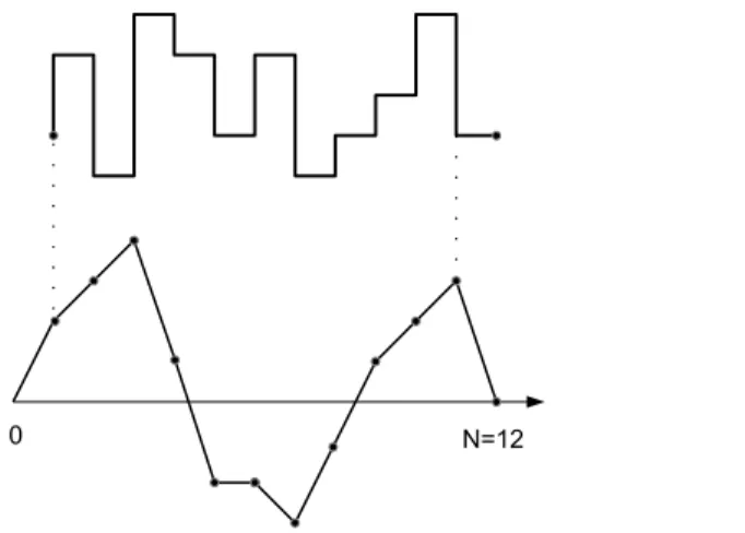
and (see Fig. 4) we denote byTN the one-to-one correspondence that mapsVN,L N onto LN,Las
TN(V )i= ( 1)i 1Vi for all i2 {1, . . . N}. (3.1) Coming back to the proof of (1.7) we recall (1.1–1.5) and we note that 8x, y 2 Z one can writex^ y =e 1
2(|x| + |y| |x + y|). Hence, for > 0andL2 N, the partition function in (1.5) becomes ZL, = L X N =1 X l2LN,L l0=lN +1=0 exp⇣ N X n=1 |ln| 2 N X n=0 |ln+ ln+1| ⌘ = c e L L X N =1 c e N X l2LN,L l0=lN +1=0 N Y n=0 exp⇣ 2|ln+ ln+1| ⌘ c . (3.2)
Then, since forl2 LN,Lthe increments(Ui)N +1i=1 ofV = (TN) 1(l)in (3.1) necessarily satisfyUi := ( 1)i 1(li 1+ li), one can rewrite (3.2) as
ZL, = c e L L X N =1 c e N X V2VN,L N P (V ), (3.3)
which immediately implies (1.7). A useful consequence of formula (3.3) is that, once conditioned on taking a given number of horizontal stepsN, the polymer measure is exactly the image measure by theTN transformation of the geometric random walkV conditioned to return to the origin afterN + 1steps and to make a geometric areaL N, i.e.,
PL, l2 · | Nl= N = P TN(V )2 · | VN +1= 0, GN = L N . (3.4)
4 Scaling Limits in the critical phase
In this section we will prove the items (2) of Theorems 2.1 and 2.2 which correspond to the critical case( = c). To simplify notations, we shall write instead of cuntil the end of this proof. In Section 4.1 below, we first exhibit a renewal structure for the underlying geometric random walk, based on “excursions”. Then we state a local limit theorem for the area of such an excursion. This Theorem has been proven recently in [12]. With these tools in hand we will be able to prove Theorem 2.1 (2) in Section 4.2 and Theorem 2.2 (2) in Section 4.3. Finally, in Section 4.4, we identify the limiting law of the rescaled horizontal extension obtained in Section 4.3 with that of the Brownian stopping timeg1under a proper conditioning.
0 N=12
Figure 4: An example of a trajectoryl = (li)11i=1withl1= 2, l2= 3, l4= 4. . . is drawn on the upper picture. The auxiliary random walkV associated withl, i.e.,(Vi)12i=0 = (T11) 1(l) is drawn on the lower picture withV1= 2, V2= 3, V4= 4 . . .
4.1 Preparations The renewal structure
We introduce a sequence of stopping times(⌧k)k2Nwhich are similar to ladder times. To be more specific we set⌧0= 0and
⌧k+1= inf{i > ⌧k : Vi 16= 0andVi 1Vi 0} . (4.1) To these we associate, forj2 N, the length of thejth inter-arrival of(⌧k)k2N, i.e.,
Nj= ⌧j ⌧j 1 (j 1) , (4.2)
and the associated geometric area
Aj= V⌧j 1 +· · · + V⌧j 1 (j 1) . (4.3)
We let⌧ = ⌧1= N1. Let us observe thatA1= G⌧ 1(V ). For simplicity, we will drop theV dependency ofGin what follows.
Now, we state the main result of this section, and the remaining part of this section is devoted to its proof.
Proposition 4.1. The random variables(Ai, Ni)i 1are independent and the sequence (Ai, Ni)i 2is IID.
We shall first need to study the distribution ofV⌧. LetT be a random variable with geometric distribution with parameterp = 1 e /2that is
P (T = k) = e 2k(1 e /2) (k2 N [ {0}) ,
and letµ be the law of the associated symmetric random variable, that is µ is the distribution of"T with"independent fromT andP (" = ±1) = 1
2: µ (k) = P ("T = k) = 1 e /2 2 e 2 |k|1 (k6=0)+ (1 e /2)1(k=0). (4.4) Finally we letP ,xbe the law of the random walk starting fromV0= x2 ZandP ,µ be the law of the random walk whenV0has distributionµ .
Lemma 4.2. UnderP ,xwithx2 Zor underP ,µ , the random variableV⌧ is indepen-dent from the couple(G⌧ 1, ⌧ ). Moreover
• V⌧ =law T underP ,xwithx > 0, • V⌧ =law T underP ,xwithx < 0, • V⌧ =law µ underP ,
• V⌧ =law µ underP ,µ .
Proof. Letx > 0, y 0anda, nbe integers. UnderP ,xwe compute the probability of Tn,a,y:={G⌧ 1= a, ⌧ = n, V⌧= y}by disintegrating it with respect to the valuez > 0 taken byVn 1, i.e., P ,x(G⌧ 1= a, ⌧ = n, V⌧= y) =X z>0 P ,x(V1+· · · + Vn 1= a; Vi> 0, 1 i n 2; Vn 1= z)e 2(z+y) c = P ,x(G⌧ 1= a, ⌧ = n) e 2y, (4.5)
where can be seen as a normalizing constant for a distribution on the non negative integers, we obtain that = p andV⌧ is independent of (G⌧ 1, ⌧ )and distributed as T. Forx < 0the proof is exactly the same. Forx = 0, we take into account the possibility that the walk sticks to zero for a while. Thus, fory > 0, we partition the event{G⌧ 1 = a, ⌧ = n, V⌧ = y}depending on the valuez > 0 taken byVn 1and on the number of stepskduring which the random walks sticks to0, i.e.,
P (G⌧ 1= a, ⌧ = n, V⌧ = y) = X z>0,0kn 2 P ,x(An 1= a; Vi = 0, 0 i k; Vi > 0, k < i n 2; Vn 1= z) e 2(z+y) c := e 2y, (4.6)
where is implicitly defined by (4.6) and its dependence in a and n is omitted for simplicity. We obtain by symmetryP (G⌧ 1= a, ⌧ = n, V⌧= y) = e 2y. It is only for x = y = 0that we need to take into account positive and negative excursions, and we obtain
P (G⌧ 1= a, ⌧ = n, V⌧= 0) = 2 . Summing all these probabilities yields
= 1 e /2
2 P (G⌧ 1= a, ⌧ = n) ,
and we can conclude that the random variable V⌧ is independent from the couple (G⌧ 1, ⌧ )with distributionµ .
The final computation showing thatµ is an “invariant measure”, is straightforward:
P ,µ (V⌧ = y) = X x µ (x)P ,x(V⌧ = y) (4.7) =X x µ (x)(P ( T = y) 1(x>0)+ P (T = y) 1(x<0)+ µ (y)1(x=0)) (4.8) = . . . = µ (y). (4.9)
Proof of Proposition 4.1. The proof is based on the preceding Lemma, and uses induc-tion in conjuncinduc-tion with the Markov property. Our inducinduc-tion assumpinduc-tion is thus that the sequence(Ai, Ni)1ik is independent, that the subsequence (Ai, Ni)2ik is IID, and that the random variableV⌧kis independent of(Ai, Ni)1ik, with distributionµ . Then,
P (Ai, Ni) = (ai, ni), 1 i k + 1; V⌧k+1= y =
E h1{(Ai,Ni)=(ai,ni),1ik}PV⌧k((A1, N1) = (ak+1, nk+1); V⌧ = y) i
= µ (y)P ,µ (A⌧ 1= ak+1, ⌧ = nk+1) P ((Ai, Ni) = (ai, ni), 1 i k) , and this concludes the induction step.
Remark 4.3. The renewal structure used in the present paper is somehow reminiscent
of another renewal structure used in [33], where the author focuses on the probability that different types of integrated random walks remain positive up to an arbitrary large timen. The random walk of lawP that we consider here falls into the scope of this work. In [33], the random walk paths are decomposed into cycles containing each a positive and a negative excursion. Although the path decomposition applied in the present work is different since for instance our excursions are not necessarily of alternating signs, and although we are more focused here on establishing local limit theorems, both works rely on a particular feature associated with the type of random walks considered, namely, the statement of our Lemma 4.2 or in words, as stated in [33] “the overshoot over any fixed level is independent of the moment when it occurs and also of the walk up to this moment”.
Local limit theorem for the “excursion” area
Let us state first the theorem. Herefexstands for the density of the area of the standard Brownian excursion (see e.g. [25]).
Theorem 4.4 (Theorem 1 of [12]). With the constant C := (E (V2
1)) 1/2 and with w(x) = C fex(C x), we have
lim n!+1supa2Z
n3/2P (Gn= a| ⌧ = n) w(a/n3/2) = 0 .
Remark 4.5. From the monograph [25] we extract the asymptotics (formulas (93) and
(96)) fex(x) = e C1 x2(C2x 5+ o(x 5) (x! 0) (4.10) fex(x) = C3x2e 6x 2 (1 + o(1)) (x! +1). (4.11)
A straightforward application of the dominated convergence theorem entails that if
bn ! 1then for all⌘ > 0, 1 n2/3 X ⌘n2/3kb nn2/3 ✓ k n2/3 ◆ 3 w ✓ k n2/3 ◆ 3/2! ! Z +1 ⌘ t 3w(t 3/2) dt. (4.12)
It is easy to check from [12] that this theorem still holds when started from the “invariant measure”µ . More precisely,Rn! 0with
Rn:= sup a2Z n
3/2P
4.2 Proof of Theorem (2.1) (2)
Using the random walk representation (3.3), we obtain, since = 1, that the excess partition function is 1 c ZeL, = L X N =1 P (GN = L N, VN +1= 0) . (4.14)
Then, we partition the event {GN = L N, VN +1 = 0} with respect to r := inf{i 0 : VN i6= 0}the time length during which the random walk sticks to the origin before itsN-th step, i.e.,
1 c ZeL, = L 1X r=0 L rX N =1 P (GN = L N r, VN 6= 0, VN +1= 0) P (V1=· · · = Vr= 0) (4.15) + P (V1=· · · = VL= 0) = 1 c L + L 1X r=0 1 c rL rX N =1 P (GN = L N r, VN 6= 0, VN +1= 0) .
Then we use the fact that, for allx2 N, we haveP (U1= x) /P (U1 x) = 1 e /2, and obtain 1 c ZeL, = 1 c L + (1 e /2) L 1X r=0 1 c rL rX N =1 P (GN = L N r, VN 6= 0, VNVN +1 0) = 1 c L + (1 e /2) L 1X r=0 1 c r P (L r + 12 X) , (4.16) where X =n X kn Ak+ Nk; n 1 o (4.17) is the renewal set associated to the sequence of random variablesXk := Ak+ Nk (recall (4.1–4.3).
It is clear that we are going to obtain the same asymptotics forZeL, if we substitute P ,µ toP in the r.h.s. of (4.16), that is if we consider a true renewal process with the random variableX1having the same distribution as theXifori 2. Thus, the proof of Theorem (2.1) (2) will be a consequence of the tail estimate ofX underP ,µ in the next lemma.
Lemma 4.6. For > 0, there exists ac1, > 0such that P ,µ (X1= n) = c1, n4/3(1 + o(1)), (4.18) andc1, = (1 + e /2) q E [V2 1] 2⇡ R+1 0 x 3w(x 3 2) dx.
By applying [17, Theorem B] (see also Theorem A.7 of [19]) we deduce from (4.18) that
P ,µ (L2 X) =
sin(⇡/3) 3⇡c1, L2/3
(1 + o(1)). (4.19)
Then, it suffices to recall (4.16-4.17) to complete the proof.
Proof of Lemma 4.6. We recall that⌧1= N1and we drop the index1for simplicity. First, we use that for allj, k2 N
P ,µ (Vj+1 Vj k) P ,µ (Vj+1 Vj= k)
= 1
to write
P ,µ (X1= n) = P ,µ (A⌧ 1+ ⌧ = n) = P ,µ (A⌧ 1+ ⌧ = n, V⌧= 0) 1 1 e 2
(4.20) and then, for⌘ 2 (0, 1), we split the probability of the r.h.s. in (4.20) into two terms:
P ,µ (A⌧ 1+ ⌧ = n, V⌧ = 0) = ⌘nX2/3 k=1 P ,µ (Ak 1= n k, ⌧ = k, Vk= 0) + n X k=⌘ n2/3 P ,µ (Ak 1= n k, ⌧ = k, Vk= 0) =: un+ vn. (4.21)
From this equality, the proof will be divided into two steps. The first step consists in controllingunand the second stepvn.
Step 1
Our aim is to show that for all" > 0there exists an⌘ > 0such that
lim sup n!1 n
4/3u
n ". (4.22)
Proof. In this step, we will need an improved version of the local limit Theorem estab-lished in [6, Proposition 2.3] forVn andAn simultaneously. The proof is given in the Appendix 7.3. Proposition 4.7. sup n2N sup k,a2Z n3 P (Vn= k, An(V ) = a) 21n2g ⇣ kpn, a n3/2 ⌘ <1, (4.23) withg(y, z) = 6 ⇡e 2y2 6z2+6yz for(y, z)2 R2.
We resume the proof of (4.22) by bounding from above the probability that there exists a piece of theV = (Vi)ni=0trajectory of length smaller than n
2/3
log n with an algebraic area (seen from its starting point) that is larger thann
2 and/or that one of the increments ofV is larger than(log n)2. Thus, we setB
n:=Cn[ Dnwith Cn:=
[ i2{0,...,n 1}
{Vi+1 Vi (log n)2}and Dn := [ (j1,j2)2Jn {Aj1,j2 Vj1(j2 j1) n 2, Vj1 0} where Jn = (j1, j2) 2 {0, . . . , n}2: 0 j2 j1 n 2/3 log n andAs,t = Pt 1
i=sVi. Then, for each(j1, j2)2 Jnwe apply Markov property atj1and we get
P ,µ (Dn) X (j1,j2)2Jn P (Aj2 j1 n 2). (4.24)
Since underP ,µ , the random variableV1has small exponential moments, there exists a constantC > 0such that
P ,µ ✓ sup 1kn|Vk| xn ◆ 2e Cnx^x2 (x 0, n2 N) . (4.25) We note thatAj2 j1 n
2 impliesmax{|Vi|, i = 1, . . . , j2 j1} 2(j2nj1) so that finally we can use (4.25) to prove that there existsC00> 0such that
sup (j1,j2)2Jn P (Aj2 j1 n 2) P ✓ sup 1jn2/3/ log(n)|V j| n 1/3 2 log(n) ◆ 2e C00log(n)3, (4.26)
which (recall (4.24)) suffices to claim thatP ,µ (Dn) = o(1/n4/3). Moreover,P ,µ (V1 (log n)2)
ce 2log(n) 2
suffices to conclude that P ,µ (Cn) = o(1/n4/3) which, in turn, implies thatP ,µ (Bn) = o(1/n4/3).
At this stage, for k ⌘n2/3, we can partition the set
{Ak 1 = n k, ⌧ = k, Vk = 0} depending on the indices at which a trajectory passes abovepkfor the first and the last time. Thus, we set⇠p
k= inf{i 0 : Vi p k}and⇠bp k= max{i k : Vi p k}. We also consider the positions ofV at⇠p
kand⇠bpk and the algebraic areas belowV in-between 0 and ⇠p
k, ⇠pk and⇠bpk as well as ⇠bpk and k. Thus, we set ¯t = (t1, t2), x = (x¯ 1, x2), ¯ a = (a1, a2)and we write {Ak 1= n k, ⌧ = k, Vk= 0} = [(¯t,¯x,¯a)2Gk,nYn,k(¯t, ¯x, ¯a), (4.27) with Yn,k(¯t, ¯x, ¯a) := n ⌧ = k, ⇠p k = t1, b⇠pk = k t2, (4.28) Vt1 = x1, Vk t2 = x2, Vk = 0, At1 = a1, At1,k t2 = n k a1 a2, Ak t2,k= a2 o , and with Gk,n= n (¯t, ¯x, ¯a)2 N6: 0 t1 k t2 k 1, 0 a1 k3/2, 0 a2 k3/2, x1 p k, x2 p ko. (4.29) Then we set e Gk,n= (¯t, ¯x, ¯a)2 Gk,n: k t1 t2 n 2/3 log n or x1 p k > log(n)2 , (4.30) and we note that if(¯t, ¯x, ¯a)2 [⌘nk=12/3Gek,n, then eitherx1
p
k (log n)2, which implies in particularYn,k(¯t, ¯x, ¯a)⇢ Cn, orx1
p
k + (log n)2and then
At1,k t2 Vt1(k t1 t2) = n k a1 a2 x1(k t1 t2) (4.31) n k 3k3/2 (log n)2k
n ⌘n2/3 3⌘3/2n log(n)2⌘n2/3 n 2,
provided⌘ is chosen small enough. Thus,Yn,k(¯t, ¯x, ¯a)⇢ Dnso that [⌘nk=12/3[(¯t,¯x,¯a)2 eGk,nYn,k(¯t, ¯x, ¯a)⇢ Bn. Clearly, for k n2/3/ log(n)we have G
k,n = eGk,n so that we should simply focus on bounding from above
P ,µ ⇣ [⌘nk=2/3n2/3 log n [(¯t,¯x,¯a)2Gk,n\ eGk,nYn,k(¯t, ¯x, ¯a) ⌘ . Pickn2/3/ log n k ⌘n2/3and(¯t, ¯x, ¯a)
2 Gk,n\ eGk,n. By applying Markov property att1andk t2and by applying time reversibility betweenk t2andk, we can write
with
S1= P ,µ (⌧ > t1, Vt1 = x1, ⇠pk = t1, At1 = a1)
S2= P ,x1(⌧ > k t1 t2, Vk t1 t2 = x2 x1, Ak t1 t2 = n k a1 a2) S3= P (⌧ > t2, Vt2 = x2, ⇠pk = t2, At2 = a2). (4.33) Since we are looking for an upper bound of the r.h.s. in (4.32), we can remove the restriction{⌧ > k t1 t2}inS2and write
S2 P (Vk t1 t2 = x2 x1, Ak t1 t2 = n k a1 a2 x1(k t1 t2)). (4.34) Therefore, it remains to bound
⌘n2/3 X k=n2/3/ log n X (¯t,¯x,¯a)2Gk,n\ eGk,n S1S2S3
and we recall (4.34) and Proposition 4.7 that yieldS2 eS2+ bS2withSe2=(k tC11t2)3 and b S2=(k tC12t2)2 g( x2 x1 p k t1 t2, n k a1 a2 x1(k t1 t2) (k t1 t2)3/2 ), (4.35) withg(y, z) = 6⇡e 2y2 6z2+6yz 6
⇡e 3
2z
2
. We recall (4.31) and we write
b S2 (k tC12t2)2e 3 2 n2 4 2 (k t1 t2)3 , (4.36)
and then for all(¯t, ¯x, ¯a)2 Gk,n\ eGk,nwe haveSe2 C1log(n)3/n2and at the same time X (¯t,¯x,¯a)2Gk,n S1S3= X 0t1k 1 P ,µ (⌧ > t1, ⇠pk= t1, At1 k 3/2) (4.37) X 1t2k t1 P (⌧ > t2, ⇠pk = t2, At2 k 3/2),
where we have summed overx1, a1, x2anda2inGk,n. Moreover, (4.37) yields X
(¯t,¯x,¯a)2Gk,n
S1S3 P ,µ (⇠pk < ⌧0) P (⇠pk < ⌧0) C3
k , (4.38)
where we have used that the probability for the V random walk to reachpkbefore coming back to the lower half plane isO(1/pk). Thus,
⌘nX2/3 k=n2/3/ log n X (¯t,¯x,¯a)2Gk,n\ eGk,n S1Se2S3 ⌘nX2/3 k=n2/3/ log n C4log(n)3 n2k C5log(n)4 n2 = o(1/n 4/3).
It remains to bound from aboveP⌘nk=n2/32/3/ log n P (¯t,¯x,¯a)2Gk,n\ eGk,nS1Sb2S3. We rewrite (4.36) as b S2nC4/32 ⇥ n2/3 (k t1 t2) ⇤2 e 3 8 2 n2/3 k t1 t2 3 ,
and we note thatx2e 3x3/(8 2)
e x3/(4 2)
forxlarge enough. Sincek ⌘n2/3it follows thatn2/3/(k t
1 t2) n2/3/k 1/⌘so that by choosing⌘small enough we get
b S2nC4/32 e 1 4 2 n2/3 k t1 t2 3 C2 n4/3e 1 4 2 n2/3 k 3 , (4.39)
and then we use (4.37) and (4.39) to get ⌘n2/3 X k=n2/3/ log n X (¯t,¯x,¯a)2Gk,n\ eGk,n S1Sb2S3 ⌘n2/3 X k=n2/3/ log n C2 n4/3e 1 4 2 n2/3 k 3 X (¯t,¯x,¯a)2Gk,n\ eGk,n S1S3 ⌘n2/3 X k=n2/3/ log n C2 kn4/3e 1 4 2 n2/3 k 3 C2 n4/3 1 n2/3 ⌘nX2/3 k=n2/3/ log n n2/3 k e 1 4 2 n2/3 k 3 , (4.40) and the Riemann sum between brackets above converges toR0⌘(1/x)e 1/(4 2x3)dxso that the r.h.s. in (4.40) is smaller that"/n4/3as soon as⌘is chosen small enough and this completes the proof.
Step 2
Our aim is to show that for all⌘ > 0,
lim n!1n 4/3v n= (1 + e /2) r E [V2 1] 2⇡ Z +1 ⌘ x 3w(x 32) dx. (4.41) Proof. By Theorem 8 of [26] (see also Theorem A.11 of [19]) and sinceE ⇥V2
1 ⇤
< +1, we can state thatP (e⌧ = n) ⇠ Cn 3/2 with C = (E ⇥V2
1 ⇤
/2⇡)1/2and with
e⌧ = inf{i 1 : Vi 0}which may differ from⌧(recall 4.1) whenV0= 0only. In Appendix 7.2, we extend this local limit theorem to the random walk with initial distributionµ and we obtain P ,µ (⌧ = n)⇠ C⌧n 3/2 with C⌧ = (1 + e /2) r E [V2 1] 2⇡ . (4.42) Let v0n:= X ⌘n2/3kn P ,µ (⌧ = k) k 3/2w ✓ n k k3/2 ◆ .
We recall the definition ofRn in (4.13) and we write |vn v0n| X ⌘n2/3kn P ,µ (⌧ = k) k 3/2Rk C0R⌘n2/3 X ⌘n2/3kn k 3 C00R⌘n2/3 1 ⌘2n4/3 = o(n 4/3) . (4.43)
We can establish by dominating convergence (see Remark 4.5) that
n4/3v0n! C⌧ Z +1
⌘
t 3w(t 3/2) dt. (4.44)
By putting together (4.43), (4.44) we obtain (4.41) and this completes the proof.
4.3 Proof of Theorem 2.2 (2)
Let(Ui)1i=1be the sequence of inter-arrivals of a1/3-stable regenerative set1Ton [0, 1], conditioned on12 Tand denote by(Ui)1
i=0its order statistics. Let(Yi)1i=1 be an
1We refer to [9, Appendix A] for a self-contained introduction of the↵-stable regenerative sets on[0, 1](see
also [2]). In fact, it is useful to keep in mind that such a set is the limit in distribution of the set ⌧
N\ [0, 1]
when⌧is a regenerative process onNwith an inter-arrival lawKthat satisfiesK(n)⇠ L(n)/n1+↵and with
La slowly varying function. The alpha-stable regenerative set can also be viewed as the zero set of a Bessel bridge on[0, 1]of dimensiond = 2(1 ↵).
IID sequence of continuous random variables, independent of(Ui)1i=0, with density dPY1(x)/ 1 x3w 1 x3/2 1R+(x). (4.45)
We are first going to prove that
lim L!+1 Nl L2/3 =law +1 X i=1 Yi(Ui)2/3=law +1 X i=1 YiU2/3i , (4.46) where the second identity in law in (4.46) is obvious and then we shall identify the distribution ofP+1i=1YiU2/3i with the distribution ofg1conditionally onBg1 = 0.
We recall (4.1–4.3) and we consider the i.i.d. sequence of random vectors(Ni, Ai)1i=1 and we recall thatXi= Ni+ Aifori2 N. We recall that, underP , the first excursion has lawP ,0and the next excursions have lawP ,µ . Let us setSn = X1+· · · + Xnand vL:= max{i 0 : Si L}. We recall (4.17) and we consider the sequence
(Ni, Ai, Xi)vi=1L
under the law P (·|L 2 X). We denote by Xr1 · · · XrvL the order statistics of (Xi)vi=1L such that ifXri = Xrj and i < j then ri < rj. To simplify notations we set (Ni, Ai, Xi) = (N
ri, Ari, Xri)fori2 {1, . . . , vL}.
To begin with, we will prove (4.46) subject to Propositions 4.8 and Claim 4.9 below. Then, the remainder of this section will be dedicated to the proof of Propositions 4.8 and Claim 4.9. Proposition 4.8. lim L!1 PvL i=1Ni L2/3 =Law 1 X i=1 Yi(Ui)2/3. (4.47)
Claim 4.9. For = c,t2 [0, 1)andLlarge enough,
PL, ✓ Nl L2/3 t ◆ = tL2/3 1 X r=0 ⇠r,LP ✓ r +PvL r+1 i=1 Ni L2/3 t | L r + 12 X ◆ (4.48) with ⇠r,L= (1 e /2)P (L r + 1 2 X) cr 1ZeL, , r2 {0, . . . , L}. (4.49) Pickt 2 [0, 1)and" > 0. Combining (4.49) with (4.16) and Theorem 2.1 (2), we obtain that
L 1 X r=1
⇠r,L= 1 + o(1). (4.50)
Moreover, by combining (4.49) with (4.18) and Theorem 2.1 (2) we can claim that there exists anr"2 Nsuch that, providedLis chosen large enough, we havePr r"⇠r,L ". Thus, with (4.50) we have also thatPr"
r=0⇠r,L2 [1 ", 1]. Then, we use Claim 4.9 and we apply Proposition 4.8 to each probability indexed byr2 {1, . . . , r"}in the r.h.s. of (4.48) to conclude that, forLlarge enough
(1 ")P ✓X1 i=1 Yi(Ui)2/3 t ◆ " PL, ⇣ Nl L2/3 t ⌘ 2" + P ✓X1 i=1 Yi(Ui)2/3 t ◆ , (4.51) which completes the proof of (4.46).
Proof of Proposition 4.8
To begin with, let us distinguish between thekexcursions associated with the firstk
variables of the order statistics(Xi)vL
i=1and the others, i.e., PvL i=1Ni L2/3 = Ak,L+ Bk,L (4.52) with Ak,L= k X i=1 Ni L23 and Bk,L= vL X i=k+1 Ni (Xi)23 ⇣ Xi L ⌘2 3 . (4.53)
Then, the proof of Proposition 4.8 will be deduced from the following two steps.
Step 1 Show that for allk2 Nand underP (· | L 2 X),
lim L!1Ak,L=law Pk i=1Yi(Ui) 2 3. (4.54)
Step 2 Show that for all" > 0,
lim
k!1lim supL!1 P (Bk,L "|L 2 X) = 0.
(4.55) Before proving (4.54) and (4.55), we need to settle some preparatory lemmas. To begin with we letF be the distribution function ofX underP ,µ that isF (t) = P ,µ (X t) fort2 RandF 1its pseudo-inverse, that isF 1(u) = inf
{t 2 R: F (t) u}foru2 (0, 1).
Lemma 4.10. There existsC > 0such that
F 1(u)⇠ C
(1 u)3 asu! 1 . (4.56)
Proof. The proof is a straightforward consequence of (4.18).
Recall (4.45). The next lemma deals with the convergence in law, asm! 1, of the horizontal extension of an excursion renormalized bym2/3and conditioned on the area of the excursion being equal tom.
Lemma 4.11. For all > 0and allm2 Nwe consider the random variable N
m2/3 under the lawsP ,a(·|X = m)witha2 {0, µ }. We have
lim m!1
N1
m2/3 =LawY1, (4.57)
and also that the sequence E ,a mN2/3 X = m m2Nis bounded.
Proof. With the help of Theorem (4.4) we can use the following equality
P ,µ (N = n X = m) = P ,µ (A = m n N = n)
P ,µ (N = n) P ,µ (X = m)
, (4.58)
combined with (4.42) and (4.18), to claim that there exists aD > 0such that
P ,µ (N = n X = m) = D m4/3 n3 w ⇣ m n n3/2 ⌘ +m 4/3 n3 ("1(m) + "2(n)) , (4.59) with"1(m)and"2(n)vanishing asm, n! 1.
To display an upper bound for the sequence E ,µ mN2/3 X = m m2N it suffices of course to consider E ,µ ⇣ N m2/31{N m2/3} X = m ⌘ = m X n=m2/3 n m2/3P ,µ (N = n X = m) (4.60) = m X n=m2/3 Dm 2/3 n2 w ⇣ m n n3/2 ⌘ + m X n=m2/3 m2/3 n2 ("1(m) + "2(n)), where we have used (4.59). Since the second term in the r.h.s. in (4.60) clearly vanishes as m ! 1, we focus on the first term and sincew is uniformly continuous because
s! w(s)is continuous on[0,1)and vanishes ass! 1, we can write the first term as a Riemann sum that converges toR11 D
x2 w( 1
x3/2)dxplus a rest that vanishes asm! 1 and this gives us the expected boundedness.
Similarly, the convergence in law is obtained by pickingt2 [0, 1)and by writing
P ,µ ⇣ N1 m2/3 t X = m ⌘ =:eum+evmwhere e um= 1 P ,µ (X = m) ⌘ m2/3 X k=1 P ,µ (Ak 1= m k, ⌧ = k) (4.61) evm= 1 P ,µ (X = m) tm2/3 X k=⌘ m2/3 P ,µ (Ak 1= m k, ⌧ = k) , (4.62)
where ⌘ 2 (0, t). We note easily thatuem = [(1 e /2) P ,µ (X = m)] 1um with um defined in (4.21). Therefore, (4.18) and (4.22) tell us thateumcan be made arbitrarily small provided⌘is small enough andmlarge enough. Thus, it remains to deal withevm, which, with the help of (4.18) is treated as the second term in the r.h.s. in (4.21). Thus, (4.41) tells us that there exists aD > 0such thatlimm!1evm=R
t ⌘Dt
3w(t 3/2) dtand this suffices to complete the proof of (4.57).
Lemma 4.12. For > 0and" > 0, there exists ac"> 0such that forL2 N,
P (vL c"L1/3) ". (4.63)
Proof. Since underP only the first excursion has lawP ,0and the othersP ,µ the proof of (4.63) will be complete once we show for instance that forclarge enough and
L2 N
P ,µ (max{Xi, i cL1/3} L) ". (4.64) We recall that, if( i)cL
1/3 +1
i=1 are the partial sums of( i)cL 1/3
+1
i=1 a sequence of IID expo-nential random variables with parameter1, we can state that
max{Xi, i cL1/3} =law F 1 ecL1/3/ cL1/3+1 . (4.65) withecL1/3 = 2+· · · + cL1/3+1. Thus we can rewrite the l.h.s. in (4.64) as
P ✓ F 1✓ ecL1/3 cL1/3+1 ◆ L ◆ = P F 1(DL)(1 DL)3 L(1 DL)3 , (4.66) withDL= ecL1/3/ cL1/3+1. After some easy simplifications we rewrite (4.66) as
P ✓ 1 ⇥F 1 DL)] 1 3(1 D L) cL 1/3+1 L13 ◆ , (4.67)
and then we use the law of large number combined with Lemma 4.10 to claim that, as
L! 1, the r.h.s. in (4.67) converges toP ( 1 c C1/3), which can be made arbitrarily small forclarge (note thatCis the positive constant appearing in Lemma 4.10). This completes the proof of the lemma.
Lemma 4.13. For every > 0, there exists a M > 0 such that, for every function
G :P({0, . . . , L/2}) ! R+, we have
E hG X\⇥0,L2⇤ L2 Xi M E hG X\⇥0,L2⇤ i. (4.68) Proof. We compute the Radon Nikodym density of the image measure ofP (·|L 2 X)by
X\ [0, L/2]w.r.t. its counterpart without conditioning. For0 = y0< y1<· · · < ym L/2 we obtain P (⌧\ [0,L 2] = (y0, . . . , ym)|L 2 X) P (⌧\ [0,L 2] = (y0, . . . , ym)) := GL(ym) + KL(ym), with GL(y) = PL/4 n=0P ,µ (n2 X) P ,µ (X = L n y) P (L2 X) P ,µ (X L2 y) , KL(y) = PL/2 n=L/4P ,µ (n2 X) P ,µ (X = L n y) P (L2 X) P ,µ (X L2 y) . (4.69)
Note that, for y = 0, the termsP ,µ (X = L n y)and P ,µ (X L2 y) in the expression ofGL(y)andKL(y)should be replaced byP ,0(X = L n y)andP ,0(X
L
2 y), respectively. However, this does not change anything in the sequel and this is why we will focus ony > 0. It remains to prove thatGL(y)andKL(y)are bounded above uniformly inL2 Nandy2 {0, . . . , L/2}. We will focus onGL sinceKL can be treated similarly.
The constantsc1, . . . , c4below are positive and independent of L, n, y. By recalling (4.18) and sinceL n y L/4whenn2 {0, . . . , L/4}we can claim that in the numerator ofGL(y), the termP ,µ (X = L n y)is bounded above byc1/L4/3 independently ofn while (4.19) implies thatPL/4n=0P ,µ (n 2 X) c2L1/3. Let us now deal with the denominator: (4.19) tell us thatP ,µ (L2 X) c3/L2/3while (4.18) gives
P ,µ (X L2 y) P ,µ (X L2) Lc1/34 .
As a consequence,GL(y)is bounded above uniformly inL2 Nandy2 {0, . . . , L/2}. We resume the proof of Proposition 4.8.
Proof of Step 1 (4.54)
The proof of Step 1 will be complete once we show that
lim l!1 ✓⇣X1 L ⌘2 3 , . . . ,⇣ X k L ⌘2 3 , N 1 (X1)23 , . . . , N k (Xk)23 ◆ =Law(U1, . . . , Uk, Y1, . . . , Yk). (4.70) To obtain this convergence in law, we considerg1, . . . , gk that are real Borel and bounded functions. We consider alsot 2 Nand(xi)ti=1 a sequence of strictly positive integers satisfyingx1+· · · + xt= Lwith an order statisticsxr1 · · · xrt. The key observation is that, by independence of the(Ni, Xi)i2N, we have
E Yk j=1 gj ⇣ Nj (Xj)23 ⌘ Xi= xi, 1 i t = k Y j=1 E , 0 1{rj =1}+µ 1{rj >1} gj ⇣ N X23 ⌘ X = xrj . (4.71)
We considerf1, . . . , fk, g1, . . . , gk that are real Borelian and bounded functions and we use (4.71) to observe that
E Yk j=1 fj ⇣⇥Xj L ⇤2 3⌘g j ⇣ Nj (Xj)23 ⌘ L2 X (4.72) = E Yk j=1 fj⇣⇥X j L ⇤2 3⌘E , 0 1{rj =1}+µ 1{rj >1} h gj ⇣ N X23 ⌘ X = Xji L2 X .
Because of Lemma 4.6, we can assert that, underP (·|L 2 X)the random set(X/L)\[0, 1]
converges in law towardsU, i.e., the1/3regenerative set on[0, 1]conditioned on12 U
(the latter convergence is proven e.g. in [9], Proposition A.8). As a consequence X1
L , . . . , Xk
L converges in law towards(U
1, . . . , Uk)which implies thatX1, . . . , Xk tend to1in probability and therefore we can use Lemma 4.11 to show that the l.h.s. in (4.72) tends to (asL! 1) k Y j=1 E⇥gj(Y )⇤E hYk j=1 fj(Uj) i . (4.73)
Thus, the proof of Step 1 is complete.
Proof of Step 2 (4.55)
One easily check that, underP ,µ (·|L 2 X), the following reversibility holds true, i.e., (Ni, Ai, Xi)vi=1L =law(N1+vL i, A1+vL i, X1+vL i)
vL
i=1. (4.74)
However, (4.74) is not true underP (·|L 2 X)since(N1, A1, X1)does not have the same law has its counterparts indexed inN \ {1}. For this reason, in the first part of the proof we will show that proving (4.55) underP ,µ (·|L 2 X)yields that (4.55) also holds true underP (·|L 2 X)and then, in the second part of the proof, we will show that (4.55) is true underP ,µ (·|L 2 X).
Part 1: (4.55) under P ,µ (·|L 2 X) yields (4.55) under P (·|L 2 X). Let us first note that ifV := (Vi)1i=0is a random walk of lawP , thenV := (Ve i+1)1i=0 is random walk of lawP ,⌫ where⌫ is the law of an increment of the random walk (recall (1.6)), i.e.,
⌫ (k) = e 2|k|
c , k2 Z. (4.75)
The Radon-Nikodym density ofP ,⌫ with respect toP ,µ is a function ofV0, i.e., dP ,⌫ dP ,µ (V ) = 2 1 + e 1{V06=0}+ 1 1 + e 1{V0=0}, V = (Vi) 1 i=02 ZN0, (4.76)
and therefore, it is bounded above and below by two positive constants. Consequently, proving (4.55) underP ,µ (·|L 2 X)or under P ,⌫ (·|L 2 X) is equivalent. As a con-sequence, the first part of the proof will be complete once we show that (4.55) under
P ,⌫ (·|L 2 X)yields (4.55) underP (·|L 2 X). To that purpose, we considerV = (Vi)1i=0 a random walk of lawP and we recall thatV := (Ve i+1)1i=0is a random walk of lawP ,⌫ . It turns out in this case that
where the sequence ( eNi, eAi, eXi)1i=1 is defined with Ve as in (4.1-4.3) and (4.17) while (Ni, Ai, Xi)1i=1 is defined with V. Obviously, (4.77) yields that vL = evL 1 and that
{L 2 X} = {L 12 eX}. We letXeer1 · · · XeervL be the order statistics of( eXi) vL i=1and we can write e Bk 1,L 1:= evL 1 X i=k e Neri (L 1)2/3 vL X i=k Neri L2/3 1 (L 1)2/3, (4.78)
where, in the last inequality of (4.78), the term1/(L 1)2/3is subtracted to take into account the fact thatNe1= N1 1(recall (4.77)) which plays a role if1 /2 {er1, . . . ,erk 1}. At this stage, it remains to note that if1 /2 {r1, . . . , rk} or if1 2 {r1, . . . , rk}andX1 > Xrk then {r1, . . . , rk} = {er1, . . . ,erk}. Otherwise, if1 2 {r1, . . . , rk} andX1 = Xrk then {r1, . . . , rk} \ {1} = {er1, . . . ,erk 1}so that in any case (4.78) yields
e Bk 1,L 1 vL X i=k+1 Nri (L 1)2/3 1 (L 1)2/3 Bk,L 1 (L 1)2/3,
which is sufficient to conclude that (4.55) under P ,⌫ (·|L 2 X) yields (4.55) under P (·|L 2 X).
Part 2: proof of (4.55) under P ,µ (·|L 2 X). Reversibility yields that, under P ,µ (·|L 2 X),
(Ni, Ai, Xi)vi=1L =law(N1+vL i, A1+vL i, X1+vL i) vL i=1.
We setvL/2 := max{i 1 : Si L/2}andv0L/2:= vL min{i 1 : Si L/2}such that vL/2andvL/20 have the same law and
(Ni, Ai, Xi) vL/2
i=1 =law(N1+vL i, A1+vL i, X1+vL i) v0L/2
i=1 . (4.79)
We also denote by(Nmid, Amid, Xmid)the features of the excursion containingL/2in case ⌧vL/2 < L/2. In case⌧vL/2= L/2, we set(Nmid, Amid, Xmid) = (0, 0, 0).
By applying Lemmas 4.12 and 4.13 and time reversibility we can state that by choosingclarge enough, the quantityP ,µ
⇣
vL/2, vL/20 cL1/3|L 2 X ⌘
is arbitrary close to1uniformly inL. Thus, we set
Hc,L={L 2 X} \ {vL, v0L cL1/3},
and Step 2 will be complete once we show that, for eachc > 0and" > 0.
lim
k!1lim supL!1
P ,µ (Bk,L "|Hc,L) = 0. (4.80) By Markov’s inequality Step 2 will be a consequence of
lim
k!1lim supL!1
E ,µ [Bk,L|Hc,L] = 0. (4.81)
We recall (4.53) and we computeE (Bk,L|Hc,L)by conditioning on (Xi, i2 N)as we did in (4.71). We recall thatHc,Lis (Xi, i2 N)-measurable.
E (Bk,L|Hc,L) = E ,µ 2 4 vL X i k+1 E ,µ N X23 X = Xi ✓Xi L ◆2 3 Hc,L 3 5 , (4.82)
but then, we can use Lemma 4.11 which allows us to bound by M > 0 each term
E ,a⇥N/X 2
thatP ,µ (Hc,L|L 2 X) ⌘uniformly inLwe can claim that the proof will be complete once we show that
lim k!1lim supL!1 E ,µ 2 4 vL X i k+1 ⇣ Xi L ⌘2 3 1{vL/2cL1/3}1{v0 L/2cL1/3} L2 X 3 5 = 0. (4.83) We note that, underP ,µ (·|L 2 X) we have necessarilyXi L/kfori k + 1. For simplicity we assume thatk2 2Nand we denote by( eX1, . . . , eXvL/2)the order statistics of the variables(X1, . . . , XvL/2)and by( ¯X
1, . . . , ¯Xv0
L/2)the order statistics of the variables (XvL, XvL 1, . . . , X1+vL v0L/2). Then, we can easily note that
Pk i=1Xi
Pk/2
i=1Xei+ ¯Xiso that the expectation in (4.83) is bounded above by
2E ,µ 2 4 vL/2 X i=k/2+1 e Xi L !2 3 1{vL/2cL1/3} L2 X 3 5 + E ,µ "✓ Xmid L ◆2 3 1{XmidL/k} L2 X # , (4.84) where the factor 2 in front of the first term is a direct consequence of (4.79). The second term in (4.84) is clearly bounded by (1/k)2/3 and therefore, it can be omitted. As a consequence, it suffices to show that
lim k!1lim supL!1 E ,µ "vL/2 X i=k ⇣ eXi L ⌘2 3 1{vL/2cL1/3} L2 X # = 0. (4.85)
At this stage, we note thatPvL/2 i=k( e Xi L ) 2 31
{vL/2cL1/3}only depends on the random set of pointsX\ [0, L/2]and this allows us to use Lemma 4.13 to claim that proving (4.85) without the conditioning by{L 2 X}is sufficient. Therefore, we only need to estimate the quantity E ,µ 2 4 cLX1/3 i=k ⇣ Xi L ⌘2 3 3 5 , where(X1, . . . , XcL1/3
)is the order statistics of(X1, . . . , XcL1/3)underP without any conditioning. We recall that, if( i)cL
1/3 +1
i=1 are the partial sums of( i)cL 1/3
+1
i=1 a sequence of IID exponential random variables with parameter1, then it is a standard fact that
(Xi)cL1/3 i=1 =law ✓ F 1 cL1/3+1 i cL1/3+1 ◆cL1/3 i=1 . (4.86)
Moreover, by Lemma 4.10, we can claim that there exists aM > 0such thatF 1(u) M/(1 u)3for allu2 (0, 1)and consequently
E ,µ 2 4 cL1/3 X i=k ⇣ Xi L ⌘2 3 3 5 ML2/32/3 cL1/3 X i=k E ✓ cL1/3+1 i 2◆ , (4.87)
but then we can bound from above the general term in the sum of the r.h.s. in (4.87) by
E ✓ cL1/3+1 i 2◆ = c2L23E ✓ cL1/3+1 cL1/3 2 1 i 2◆ c2L2 3E ✓ cL1/3+1 cL1/3 4◆1 2 E ✓ 1 i 4◆1 2 . (4.88)
It remains to point out, on the one hand, that by the law of large numberE⇣h cL1/3 +1 cL1/3
i4⌘ converges to1asL ! 1and, on the other hand, that for alli2 N \ {0}, i follows a Gamma distribution of parameter(i, 1)which entails that fori 5,E⇣h1ii4⌘= (i 5)!(i 1)!. Consequently, we can use (4.87) and (4.88) to complete the proof of Step 2.
Proof of Claim 4.9
We use again the random walk representation (3.3), and since = 1, we obtain
PL, ⇣ Nl L2/3 t ⌘ = c e ZL, tL2/3 X N =1 P (GN = L N, VN +1= 0) . (4.89) Similarly to what we did in (4.14–4.16), we partition the event{GN = L N, VN +1= 0} depending on the lengthron which the random walk sticks at the origin before its right extremity, that is PL, ⇣ Nl L2/3 t ⌘ = tL2/3 1 X r=0 (1 e /2) cr 1ZeL, tL2/3 r X N =1 P (GN = L N r, VN 6= 0, VNVN +1 0) = tL2/3 1 X r=0 ⇠r,LP ✓r + N 1+· · · + NvL r+1 L2/3 t | L r + 12 X ◆ , (4.90) where we recall the definition of⇠r,Lin (4.49). This ends the proof of Claim 4.9.
4.4 Identifying the distribution oflimL!+1LN2/3l
LetB be a standard Brownian motion on the line; we consider its geometric area and its continuous inverse
Gt(B) = Z t
0 |B
s| ds , ga= inf{t > 0 : Gt(B) = a} . (4.91)
We aim to identify formally the distribution oflimL!+1LN2/3l =lawP+i=11YiU2/3i with the distribution ofg1conditionally onBg1= 0.
Step 1: Identifying the distribution ofY1
We shall show thatY1is distributed as the extension of a Brownian excursion normalized by its area. The Brownian excursion distribution is⇡1= P0,03,1the law of the Bessel bridge of dimension 3 and length1. We may view this law as the distribution of the excursion conditioned to have length (extension)1. This is an easy consequence of It’s description of the excursion measure (see [30, Theorem 4.2] or [28, section 2]). Indeed let⇣(!)be the extension (length,duration) of an excursion
⇣(!) := inf{t > 0 : !(t) = 0} , (4.92)
and⇡r= P0,03,r be the law of the Bessel bridge of dimension3over[0, r]. Then undern+, the positive excursion measure,⇣has density 1
2p2⇡r3 and we have n+( ) = Z +1 0 ⇡r( ) dr 2p2⇡r3 = Z +1 0 ⇡r( ) n+(⇣2 dr) . (4.93) The usual scaling operator issc(!)(t) = p1c!(ct)and we have⇡r(F (!)) = ⇡1(F (s1/r(!))). Thus, if ⌫(!) = s⇣(!)(!) is the operator that normalizes the length of the excursion,
⇣(⌫(!)) = 1, then we have an independence between the length of an excursion and its shape, easily deduced from (4.93): for any positive measurableF,
n+(F (⌫(!)) (⇣(!)) = ⇡1(F (!))n+( (⇣)) . If we consider now instead of the extension the area
A(!) = Z +1 0 !(s) ds = Z ⇣(!) 0 !(s) ds , (4.94)
then the operator that normalizes the area of an excursion is⌘(!) = sA(!)2/3(!)and we can establish using scaling again that there exists a probability Adefined on excursions such that A(A(!) = 1) = 1and that satisfies for every positive measurableF, :
n+[F (⌘(!)) (A(!))] = A(F (!))⌘+( (A(!))) . (4.95) It is natural to say that A is the law of the Brownian excursion normalized by its area and it is just a matter of playing with scaling again to show that Y1 of density proportional to 1
x3w(x3/21 )is distributed asC 2/3
⇣(!)under A.
Step 2: A Brownian construction of a 1
3-stable regenerative set and a formal
identity in law.
Observe that if(⌧t, t 0) is the inverse local time at level 0 of Brownian motion B, then by strong Markov property(G⌧t, t 0)is a subordinator. Since it has the scaling (G⌧ct, t 0) =law (c
3G
⌧t, t 0), the closure of its rangeR = {G⌧t, t 0} [ G⌧t , t > 0 is a stable 1
3 regenerative set on[0, +1[.
Therefore if(Ui)+1i=1 are the interarrivals ofT =R \ [0, 1], we have the representation {Ui, 1 i} = G⌧s G⌧s : s > 0, G⌧s 1 . (4.96) Assume that instead{Ui, 1 i} = G⌧s G⌧s : 0 < s t . Then the exponential formula for the Poisson process of Brownian excursion yields
E " exp( X i U2/3i ) # = exp ✓ 2 Z t 0 ⇣ 1 e A(w)2/3⌘n+(dw) ◆ . (4.97)
Since theYiare IID, by considering the marked Poisson process of excursion, we get E " exp( X i YiU2/3i ) # = exp ✓ 2 Z t 0 ⇣ 1 Ehe Y1A(w)2/3i⌘n +(dw) ◆ . (4.98) By the independence of the area of an excursion and its shape (we takeC = 1to simplify notations) (4.95), we obtain E " exp( X i YiU2/3i ) # = exp ✓ 2 Z t 0 (1 e ⇣(w))n+(dw) ◆ = exp ✓ Z t 0 (1 e ⇣(w))n(dw) ◆ = Ehe Pst(⌧s ⌧s )i= E⇥e ⌧t⇤ . (4.99) We extend formally this identity in law to a sum until the sum of theUi exceeds1, and we obtain formally +1 X i=1 YiU2/3i =law X s:G⌧s1 ⌧s ⌧s = g1= inf ⇢ t > 0 Z t 0 |B s| ds > 1 . (4.100)