ECONOMIC BENEFITS OF CLIMATE ACTION: THE URBAN DIMENSION

HAL Id: hal-00799234

https://hal-enpc.archives-ouvertes.fr/hal-00799234

Submitted on 11 Mar 2013

HAL is a multi-disciplinary open access archive for the deposit and dissemination of sci-entific research documents, whether they are pub-lished or not. The documents may come from teaching and research institutions in France or

L’archive ouverte pluridisciplinaire HAL, est destinée au dépôt et à la diffusion de documents scientifiques de niveau recherche, publiés ou non, émanant des établissements d’enseignement et de recherche français ou étrangers, des laboratoires

ECONOMIC BENEFITS OF CLIMATE ACTION: THE

URBAN DIMENSION

F. Grazi, H. Waisman

To cite this version:

F. Grazi, H. Waisman. ECONOMIC BENEFITS OF CLIMATE ACTION: THE URBAN DIMEN-SION. Lamia Kamal-Chaoui and Alexis Robert. Competitive Cities and Climate Change, OCDE, pp.65-77 ; 162-171, 2009. �hal-00799234�

Competitive Cities and Climate Change

Lamia Kamal-Chaoui and Alexis Robert (eds.)

JEL Classification: Q54, Q55, Q58, Q42, Q48, R00 Please cite this paper as:

Kamal-Chaoui, Lamia and Alexis Robert (eds.) (2009), “Competitive Cities and Climate Change”, OECD

Regional Development Working Papers N° 2, 2009,

OECD REGIONAL DEVELOPMENT WORKING PAPERS

This series is designed to make available to a wider readership selected studies on regional development issues prepared for use within the OECD. Authorship is usually collective, but principal authors are named. The papers are generally available only in their original language English or French with a summary in the other if available.

The opinions expressed in these papers are the sole responsibility of the author(s) and do not necessarily reflect those of the OECD or the governments of its member countries.

Comment on the series is welcome, and should be sent to either gov.contact@oecd.org or the Public

Governance and Territorial Development Directorate, 2, rue André Pascal, 75775 PARIS CEDEX 16, France.

--- OECD Regional Development Working Papers are published on

www.oecd.org/gov/regional/workingpapers

---

Applications for permission to reproduce or translate all or part of this material should be made to: OECD Publishing, rights@oecd.org or by fax 33 1 45 24 99 30.

3. ECONOMIC BENEFITS OF CLIMATE ACTION: THE URBAN DIMENSION

Simultaneously addressing stabilisation of the climate and economic growth has become a challenging task for the international policy community. This apparent trade-off has been so far discussed in two ways. The first is to measure economic growth in a way that integrates the degradation of environmental assets in the calculation of GDP. The second is to take into account the discounted long-term economic benefits of climate stabilisation, by avoiding extreme future adverse events. Both approaches entail significant measurement and valuation problems. However, findings from a regional growth model disaggregated at the metropolitan level, presented in this section, show that the trade-off between economic growth and climate policy can be actually lower when local dimensions are taken into account. Namely, policies to reduce traffic congestion and increase urban density can have a significant effect on national GHG emissions levels while allowing the local economy to grow. Also, adaptation and mitigation policies can provide important benefits in the form of reduced energy costs, increased local energy security and improved urban health. This is particularly important for city and regional governments, which can be sensitive to immediate price increases and investment costs in exchange for the less-tangible and longer-term benefits of addressing global climate change.

3.1. Impact of urban policies on global energy demand and carbon emissions

A Computable General Equilibrium (CGE) model has been used to simulate a world economy divided into macro-regions in economic interaction with metropolitan OECD areas. More precisely, this modelling exercise has been carried out by employing the spatialised version of the IMACLIM-R CGE framework (Crassous et al., 2006). IMACLIM-R allows simulating the interactions between changes in energy consumption, carbon emissions and economic growth, given a set of policies and other exogenous factors (Box 3.1).41 _{Two types of urban policies are explicitly explored: i) urban densification}42_{; and, ii)}

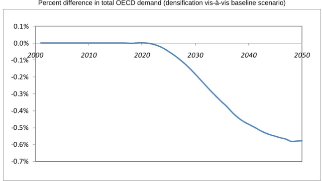
congestion charges. The results suggest that densification policies would increase people’s propensity to use public transport, from 12.9% in the baseline scenario to 14% by 2050 with densification policies. As a consequence, the volume of private transport falls across the OECD, implying a decrease in the demand for oil. If cities were to become denser, total OECD energy demand would decrease from 2020 on, and would reach 0.6% less compared to the baseline (Figure 3.1). This is in line with previous evidence that urban form affects individuals’ travel behaviour and consequently global environmental quality (Grazi et al., 2008). A similar result is obtained if congestion charges only are applied.

41. The baseline scenarios for both the IMACLIM-R and the OECD ENV-Linkages models, were made

consistent through comparable exogenous assumptions on demographic trends, labour productivity, GDP trends (as a proxy for the intensity of economic activity), fossil energy prices, energy intensity of the overall economy and carbon tax trajectories.

42. Densification indicates policies that increase the number of people per square kilometre in a given urban

area. These include restrictive and enabling policies. The former actively pursue densification through policies such as green belts, whereas the latter are those that allow activity to be drawn to the core such as public transportation systems or the elimination of distortions in the market such as taxes for deconcentration.

Box 3.1. A CGE Model of Metropolitan Economies

The impact on climate change of policies at the metro-regional scale can be modelled using a general equilibrium approach that takes into account most of the factors that influence the way in which an economic system works. In particular, computable general equilibrium (CGE) models can be used in order to simulate a world economy divided in countries and groups of countries, multiple sectors, and production and consumption functions. The approach taken in this section involves the use of IMACLIM-R model (Crassous et al., 2006; see Annex A for details). The global CGE model employed in this section has been enriched by a metropolitan module representing the metropolitan economies and their interactions with the macro-level (GRAZI and Waisman, 2009). This module was calibrated on the OECD Metropolitan Database and consistently with the assumptions in the OECD ENV-Linkages model.

The model is based on the comparison of two scenarios: one without policy changes, the so-called baseline

scenario (BS), and a climate policy scenario. The comparison of these two scenarios for each period enables

quantification of the magnitude of the changes. Two particular local policies have been tested to explore possible impacts on the economy and on carbon emissions: densification policies and congestion charges. The densification policy can be interpreted as an indirect form of intervention whose primary effect is to reduce individuals’ dependence on private transport for commuting. Densification is the increase in the number of inhabitants living in a given territorial unit, for instance, the number of inhabitants per square kilometre. In analyzing where an economy chooses to locate and under what determinants it distributes across available agglomerations, the metropolitan module in the IMACLIM-R model draws on the new economic geography approach (Krugman, 1991). The static urban agglomeration structure is described by three main determinants: locally available active population, labour productivity, and urban density. Data are taken from the OECD Metropolitan Database. The long-run mechanism through which firms (and people consequently) agglomerate is driven by an agglomeration-specific attractiveness index that encompasses three main factors: the rate of capital return, the expected volume of production and the change in absolute number of firms. Firms therefore are attracted by cities with higher capital returns (determined by labour productivity), an increase in the size of markets (given by the expected volume of production) and the presence of other firms (so that they can establish backward and forward linkages). The model also allows for migration of people among regions and cities following firms’ investment decisions. Higher-productivity cities will be able to offer higher wages and thus attract workers and skills, which completes the agglomeration cycle. Higher wages are assumed to be a compensation for workers as they need to cope with the external costs of the agglomeration, namely commuting, housing costs and local pollution.

Figure 3.1. Energy Demand with a Densification Policy

Percent difference in total OECD demand (densification vis-à-vis baseline scenario)

‐0.7% ‐0.6% ‐0.5% ‐0.4% ‐0.3% ‐0.2% ‐0.1% 0.0% 0.1% 2000 2010 2020 2030 2040 2050

Note: The line shows the difference between demand of energy once cities are denser and the baseline scenario (or business as usual).

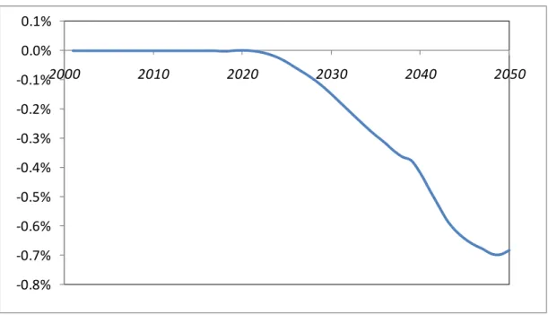
Following the implementation of densification and congestion charges, carbon emissions are reduced relative to the baseline, following a similar pattern to the one of energy demand from 2020 on (Figure 3.2). We consider the introduction of a local tax on the use of private vehicles by individuals for commuting purposes. This takes the form of a toll road of the type already implemented in some metro-regions (London and Stockholm among others). 43 _{The toll road tax can be used in second instance to finance}

metro-region densification plans, thereby lowering the cost of densification.

Figure 3.2. Carbon Emission Reductions with a Densification Policy

Percent difference in total emission reductions in OECD (densification vis-à-vis baseline scenario)

‐0.8% ‐0.7% ‐0.6% ‐0.5% ‐0.4% ‐0.3% ‐0.2% ‐0.1% 0.0% 0.1% 2000 2010 2020 2030 2040 2050

Source: Simulations from IMACLIM-R model based on the OECD Metropolitan Database.

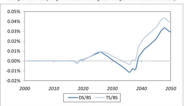
3.2. Environment and economic growth at the urban scale: from trade-offs to complementarity Densification and congestion charges are not the only effective tools to reduce energy demand and carbon emissions, however, they are important as they do not have a detrimental effect on long-term economic growth.44 _{In terms of impact on economic growth, the model generates three adjustment phases}

over time. First, an initial minor and short-lived economic expansion exists with both policies in an almost the same pattern until 2025, mainly driven by lower fuel prices as demand for oil falls. Second, economic growth becomes mildly negative after 2030 (Figure 3.3). As fuel prices fall, people find it less costly to drive again and so they increase their demand for oil and prices start to rise again, bringing about a short-lived economic contraction. Finally, a more important expansion of economic activity – more so under the

43. Such a road toll reduces average rather than marginal commuting costs by car (see Henderson, 1974 for the

underlying economics of road pricing mechanisms).

44. Note that, in the IMACLIM-R model, the explicit representation of technologies through reduced forms of

technology-rich bottom-up sub models allows for an explicit description of agents’ decisions that drive the pace and direction of technical change. Moreover, consumption and investment choices in IMACLIM-R are driven by agents’ imperfect foresight and explicit inertias on the renewal of equipments and technologies. The combination of these two features is the underlying explanation for moderate carbon abatement costs in IMACLIM-R’s policy scenarios when compared to those in other general equilibrium models.

congestion charges scenario – becomes possible around 2038 since the new increase in oil prices tends to accelerate technical change and thus spurs innovation and economic growth.

Figure 3.3. Economic Growth with Local Policies

Changes in GDP comparing densification and congestion charges vis-a-vis baseline scenario)

‐0.02% ‐0.01% 0.00% 0.01% 0.02% 0.03% 0.04% 0.05% 2000 2010 2020 2030 2040 2050 DS/BS TS/BS

Note: DS refers to Densification Scenario; BS refers to Baseline Scenario; TS refers to Tax Scenario (in turn refer to the application of congestion charges).

Source: Simulations from IMACLIM-R model based on the OECD Metropolitan Database.

Underlying these results is the fact that technology-support policies embodied in the IMACLIM-R model can reduce and even offset the economic cost of curbing carbon emissions. In this regard, the discussion on how to address the climate change problem has mainly focused on the economic impact of carbon abatement. The latter has been evaluated at 1 to 3% – depending on the discount rate used – of reduction in world GDP (cf. Stern, 2007 and OECD, 2009a). However, the OECD (2009a) acknowledges that the perceived trade-off between economic growth and mitigation policies is lower if technology-support policies are considered: first because technology-technology-support policies may help address innovation failures and boost economic growth; second because these policies postpone emission cuts until technologies become available and therefore reduce the impact on economic growth (OECD, 2009a).

In other words, the prospects of economic growth can actually be improved by providing incentives to innovation and growth. Emission reduction targets implied by climate policy bring about the need to improve processes and change products in a way that allow firms to comply with such regulations. Firms are then obliged to invest in improving their processes; many will fail to do so and perhaps be driven out of market, but many others may find new ways of doing things and in the long-run such innovation bursts will lead to greater economic progress. OECD (2009a) shows that R&D policies and technology adoption incentives are better suited than price and command-and-control (CAC) instruments for correcting specific innovation and technology diffusion failures that undermine the creation and diffusion of emissions-reducing technologies.

Assessed at the regional or local level, policies to reduce carbon emissions are less opposed to economic growth than policies designed at the aggregate level. As mentioned previously, cities are major

contributors to climate change through energy demand and on-road transportation; thus local authorities can play a part in reducing such demand and emissions by inducing changes in the way people live and commute in urban areas. Moreover, policy tools at the disposal of cities’ authorities are effective in tackling emissions by avoiding costs that are generally assumed at the macro level. Local policies that change commuting patterns – and there could be other policies to reduce emissions that are not explored with the model, such as building codes – can effectively reduce carbon emissions and, in the long run, boost economic growth through innovation. The reason for this lower trade-off at the urban level lies in the fact that more complementarities among policies and economic activities can be observed at the local than at the aggregate national level.

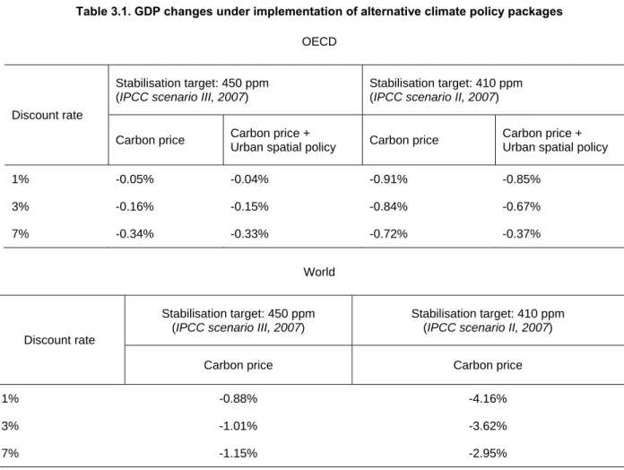
To illustrate the combined effect of climate and urban policies, an emission reduction scenario was simulated at 450 ppm (IPCC Scenario III, see Box 3.2). 45 _{In terms of carbon abatement, this scenario}

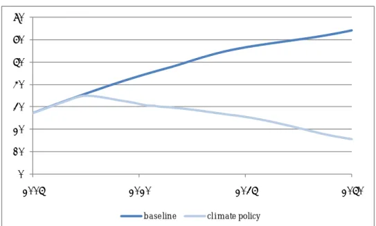
corresponds roughly to more than a three-fold reduction in world carbon emissions by 2050, compared with the baseline (from above 30 to less than 20 GtCO2). Between 2005 and 2050, world GHG emissions are reduced by roughly half. In the OECD, the abatement is even bigger in relative terms (Figure 3.4). The associated GDP losses could represent up to one-third of a percentage point for the OECD (Table 3.1).

Box 3.2. Emission Targets and Modelling of Climate Policy

When carbon emission targets set to avoid serious climate change (e.g. limiting global warming at 2° C) are compared with those considered in energy economics literature on mitigation scenarios, substantial discrepancies emerge. So far, most model assessments of mitigation costs have considered stabilisation levels of atmospheric greenhouse gas concentrations above 500 ppm CO2eq (e.g. Stern (2007) focuses on mitigation scenarios aiming at 500 to 550 ppm CO2eq). Although such stabilization levels are likely to be insufficient for keeping warming below 2°C (Meinshausen et al., 2006), they are used as a benchmark for climate-energy modelling exercises: out of 177 mitigation scenarios considered in the IPCC AR4, only six were grouped in the lowest stabilization category (corresponding to 445–490 ppm CO2eq, which is consistent with a medium likelihood of achieving the 2°C target).

The rationale behind the limited number of studies considering reduction targets that are consistent with the 2°C target is that such low stabilisation can only be attained under a number of restrictive assumptions: i) a high degree of flexibility of substitution within the energy economic system; ii) a broad portfolio of technology options (including bio-energy, other renewables and carbon capture and storage); iii) a full and immediate participation in a global mitigation effort; and, iv) the necessity of generating negative emissions.

Figure 3.4. Trends in carbon emissions under climate policy compared with the baseline

World Carbon Emissions (GtCO2) (2005-2050)

  0 10 20 30 40 50 60 70 2005 2020 2035 2050

baseline climate policy

OECD Carbon Emissions (GtCO2) (2005-2050)

  0 5 10 15 20 25 2005 2020 2035 2050

baseline climate policy

Table 3.1. GDP changes under implementation of alternative climate policy packages

OECD

Discount rate

Stabilisation target: 450 ppm (IPCC scenario III, 2007)

Stabilisation target: 410 ppm (IPCC scenario II, 2007)

Carbon price Carbon price +

Urban spatial policy Carbon price

Carbon price + Urban spatial policy

1% -0.05% -0.04% -0.91% -0.85% 3% -0.16% -0.15% -0.84% -0.67% 7% -0.34% -0.33% -0.72% -0.37% World Discount rate Stabilisation target: 450 ppm (IPCC scenario III, 2007)

Stabilisation target: 410 ppm (IPCC scenario II, 2007)

Carbon price Carbon price

1% -0.88% -4.16% 3% -1.01% -3.62% 7% -1.15% -2.95%

Notes:

For a given discount rate r, GDP losses are actualized starting from 2010, year at which the urban densification policy is expected to be set in place;

Actualized GDP losses are computed by making use of the standard formula:

2050 2010 2010(1 ) t t t GDP r − = +

∑

Note that with high discount rates both, loses and gains, in the long term, yield low discounted values. In a scenario in which loses take place at the beginning of the period and gains at the end (such as in Figure 3.3) then the discounted cumulated losses are higher the discount rate.

Source: Calculations based on the IMACLIM-R model.

For the group of OECD countries, it was possible to simulate the joint effects of implementing both a carbon price and urban spatial policies. Under the 450 ppm target, the gains from urban policies are relatively mild, although positive. If a more demanding target, such as 410 ppm, were to46 _{be reached, the}

complementarity between the two policies would be sizeable (around 0.3% of OECD GDP, when a strong discounting rate is used. The global GDP losses under the 410 ppm climate policy scenario range from 3% to greater than 4% of GDP. Although it could not be simulated at this stage by lack of data, it is likely that urban policies implemented at a global scale could generate much larger benefits.

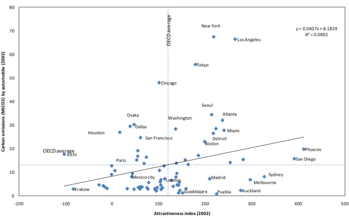
Going beyond the alleviation of carbon abatement costs, there are complementarities between carbon emission reductions and economic growth that can be found at the urban level. Using the attractiveness

46. This is the result for the OECD using the highest discount rate (7%) It is the difference between -0.72%

index that is the heart of the agglomeration dynamics in the spatialised version of IMACLIM-R model, it can be seen that a group of highly attractive metro-regions are associated with high levels of carbon emissions stemming from commuting, such as Los Angeles, New York, Seoul, Tokyo or Toronto. In contrast, a number of metro-regions combine relatively low emission levels per automobile and high attractiveness (e.g. Auckland, Madrid, and Sydney, Figure 3.5). Commuting modes could therefore be at the heart of carbon emission patterns, implying that a more intensive use of public transport may contribute significantly to reducing GHG emissions.

Figure 3.5. Attractiveness and Carbon Emissions related to Automobiles across Metro-regions

Atlanta Boston Chicago Dallas Detroit Houston Miami Los Angeles New York Phoenix San Diego San Francisco Washington Paris Krakow Madrid London _Melbourne Sydney Aichi Osaka Tokyo Seoul Auckland Guadalajara Mexico city Puebla y = 0.0407x + 8.1829 R² = 0.0802 0 10 20 30 40 50 60 70 80 ‐200 ‐100 0 100 200 300 400 500 Ca rb o n  em is si o n s  (M tC O 2 )  by  au to m o b ile  ( 2 002) Attractiveness index (2002) OE CD  av e rag e OECD average

Source: Calculations based on the IMACLIM-R model and OECD Metropolitan Database.

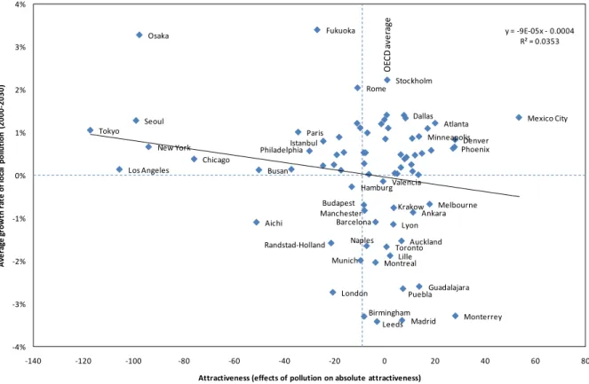
In this context, low pollution levels will increasingly be a factor driving the attractiveness of urban areas. In the next two decades, cities that could become more attractive will do so while also curbing local pollution. According to the results of the CGE model, and if current trends are sustained, cities that could experience improvements in attractiveness by 2030 include Ankara, Auckland, Barcelona, Krakow, Lille, Melbourne, Montreal, Monterrey, and Toronto; they will do so while also trimming down local pollution (Figure 3.6). Conversely, metro-regions could lose attractiveness if they continue to pollute, as in the cases of Chicago, Los Angeles, New York, Osaka, Paris, Philadelphia, Seoul and Tokyo if current trends continue.

Figure 3.6. Changes in Attractiveness and Local Pollution Emissions across Metro-regions Atlanta Chicago Dallas Denver Minneapolis Los Angeles

New York _Philadelphia Phoenix

Lille Lyon Paris Hamburg Munich Budapest Naples Rome Randstad‐Holland Krakow Madrid Barcelona Valencia Stockholm Ankara Istanbul Birmingham Leeds London Manchester Melbourne Aichi Fukuoka Osaka Tokyo Busan Seoul Auckland Montreal Toronto Guadalajara Mexico City Monterrey Puebla y = ‐9E‐05x ‐ 0.0004 R² = 0.0353 ‐4% ‐3% ‐2% ‐1% 0% 1% 2% 3% 4% ‐140 ‐120 ‐100 ‐80 ‐60 ‐40 ‐20 0 20 40 60 80 Av e ra ge  gr o w th  ra te  of  lo ca l  pol lut io n  ( 2 000 ‐2 030) Attractiveness (effects of pollution on absolute attractiveness) OE CD  av e ra ge

Source: Calculations based on the IMACLIM-R model and the OECD Metropolitan Database.

If local pollution is related to attractiveness, and the latter associated to population and firm creation, higher incomes, productivity and wages, then an environmental policy at the local level could generate economic gains. In particular, changing the urban structure by increasing cities’ density and intensifying the use of public transportation may induce both improvements in attractiveness – and therefore economic performance – and in cities’ responsiveness to climate change. As will be developed below, densification policies to respond to climate change can take the form of removing tax and development disincentives in the urban core, actively pursuing compact spatial form, and increasing mass transit networks and urban amenities in areas targeted for higher-density growth. These issues should be at the heart of the ongoing debate about a green growth strategy.

3.3. Benefits for non-climate policies

Additional local benefits resulting from emissions reductions and climate adaptation policies may also be partly responsible for a potential positive relationship between economic growth and GHG emissions reduction at the metropolitan regional level. These benefits can be grouped into five categories:

i) Public health improvements

ii) Cost savings and increased efficiency

iii) Energy security and infrastructure improvements iv) Improved quality of life

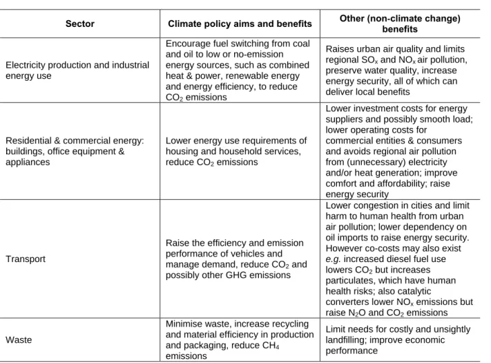
Each of these categories of benefits represent gains beyond those directly related to reduced GHG emissions or protection against climate change impacts. Table 3.2 provides an overview of some of the main co-benefits of mitigation policy in urban areas. The non-climate benefits of certain climate change policies are strong enough to warrant their implementation regardless of their impact on mitigating or adapting to climate change. In these cases they are considered “no-regrets” strategies (Hallegatte et al., 2008).

Table 3.2. Related aims and co-benefits of sector policies to reduce GHGs at urban scale

Sector Climate policy aims and benefits Other (non-climate change) _benefits

Electricity production and industrial energy use

Encourage fuel switching from coal and oil to low or no-emission energy sources, such as combined heat & power, renewable energy and energy efficiency, to reduce CO2 emissions

Raises urban air quality and limits regional SOx and NOx air pollution, preserve water quality, increase energy security, all of which can deliver local benefits

Residential & commercial energy: buildings, office equipment & appliances

Lower energy use requirements of housing and household services, reduce CO2 emissions

Lower investment costs for energy suppliers and possibly smooth load; lower operating costs for

commercial entities & consumers and avoids regional air pollution from (unnecessary) electricity and/or heat generation; improve comfort and affordability; raise energy security

Transport

Raise the efficiency and emission performance of vehicles and manage demand, reduce CO2 and possibly other GHG emissions

Lower congestion in cities and limit harm to human health from urban air pollution; lower dependency on oil imports to raise energy security. However co-costs may also exist

e.g. increased diesel fuel use

lowers CO2 but increases particulates, which have human health risks; also catalytic

converters lower NOx emissions but raise N2O and CO2 emissions Waste

Minimise waste, increase recycling and material efficiency in production and packaging, reduce CH4

emissions

Limit needs for costly and unsightly landfilling; improve economic performance

Source: Hallegatte, Stéphane, Fanny Henriet and Jan Corfee-Morlot (2008), “The economics of climate change impacts and policy

benefits at city scale: a conceptual framework”, Environment Working Papers No. 4, OECD Publishing, Paris.

Mitigating greenhouse gas emissions provides public health benefits by reducing many dangerous air pollutants (OECD, 2008a), making health benefits an important co-benefit of efforts to reduce GHG emissions in metropolitan regions. Indeed, reduction in urban air pollution is an important component of many national estimates of climate change mitigation co-benefits.47 GHG emissions reductions may benefit human health to such a degree as to offset in large part the local costs of emissions reduction (OECD, 2009b).48

Policies to reduce GHG emissions through increasing energy efficiency can result in significant reductions in energy costs. Initiatives to improve building energy-efficiency are examples of no-regrets

47. Cifuentes (1999), Davis et al. (2000) and Kunzli et al. (2000) as cited in OECD (2009b).

strategies because the energy savings achieved can compensate for the initial investment costs in as little as a few years (Hallegate et al., 2008). Policies to reduce the amount of energy already going to waste are cost-neutral if their implementation costs are compensated over time.

Both mitigation and adaptation policies can improve the security of local infrastructure and public services. Policies to mitigate greenhouse gases improve national security through reducing dependency on foreign energy sources and by reducing the risks involved in transporting highly combustible fossil fuels around the world (Schellnhuber et al., 2004). Adaptation measures can also improve the security of an area’s energy supply. For example, improving the resilience, efficiency and redundancy of energy supply networks protects against interruptions in electricity service during extreme heat events and also reduces the risk of shortfalls (peak demand outstripping supply) or intentional attacks on the system. Similarly, some infrastructure to protect coastal cities from storm surge and flood risks can be economically justified even at current sea levels (Hallegate et al., 2008).

Many of the measures that mitigate climate change and that help adapt to its effects also make cities more liveable and therefore potentially more competitive. For instance, cities that reclaim land in flood plains as part of adaptation plans can make this land available to the public as parks or recreational land. This provides an amenity to residents, removes buildings and other infrastructure from flood plains, reduces the urban heat island effect, helps control downstream flooding, provides habitat for animals, and limits water pollution by slowing storm water runoff into large bodies of water. Efforts to reduce personal vehicle use and increase use of mass transit can improve public safety and reduce traffic congestion and noise (Hallegate et al., 2008).

Adaptation to climate change and mitigation of climate change can also be complementary strategies. Adaptation focuses on expanding the ability to cope with changes in climate, whereas mitigation focuses on reducing the amount of change through reducing emissions or removing greenhouse gases from the atmosphere through sequestration. In choosing a portfolio of mitigation and adaptation measures, it may be necessary to make investment trade-offs between them. However, adaptation and mitigation can go hand in hand, for example when developing a decentralized energy system based on locally available energy sources. Here, GHG emissions may be lower, as may be the vulnerability to large-area outages from severe weather impacts.

Synergies between policies to reduce GHG emissions and adapt to expected climate change impacts are particularly important at the urban level. For example, efforts to reduce building energy demand for cooling can also reduce urban heat island effects and prevent electricity shortfalls and blackouts during extreme heat events. On the local level, adaptation and mitigation policies are deployed through the same policy sectors, including land-use planning, transportation, and building sectors, as opposed to the global scale, where mitigation and adaptation goals are designed separately. This synergy presents opportunities to design urban mitigation and adaptation policies within a consistent framework (Hallegatte et al., 2008).

REFERENCES

Crassous, Renaud, Jean-Charles Hourcade, and Olivier Sassi (2006), “Endogenous Structural Change and Climate Targets: Modeling experiments within IMACLIM-R”, The Energy Journal, Special Issue #1, International Association for Energy Economics, pp. 259-276.

Fargione, J., J. Hill, D. Tilman, S. Polasky, P. Hawthorne (2008), “Land Clearing and the Biofuel Carbon Debt”, Science, Vol. 319, No. 5867, pp.1235–1237.

Grazi, Fabio and Henri Waisman (2009), “Urban Agglomeration Economies in Climate Policy: A Dynamic CGE Approach”, CIRED Working Paper Series, CIRED (Centre International de Recherche sur l’Environnement et le Développement), Paris.

Grazi, Fabio, Jeroen van den Bergh and Jos van Ommeren (2008), “An Empirical Analysis of Urban Form, Transport, and Global Warming”, The Energy Journal, Vol. 29, No. 4, pp. 97-122.

Hallegatte, Stéphane, Fanny Henriet and Jan Corfee-Morlot (2008), “The Economics of Climate Change Impacts and Policy Benefits at City Scale: A Conceptual Framework”, Environment Working Papers No. 4, OECD, Paris.

Henderson, Vernon (1974), “Road congestion. A reconsideration of pricing theory”, Journal of Urban

Economics, Vol. 1, No. 3, pp. 346–365.

Krugman, Paul (1991), “Increasing returns and economic geography”, Journal of Political Economy, Vol. 99, No.3, pp. 483-499.

Meinshausen, M. (2006), “What does a 2°C target mean for greenhouse gas concentrations? – A brief analysis based on multi-gas emission pathways and several climate sensitivity uncertainty estimates”, in: Avoiding Dangerous Climate Change. J. S. Schellnhuber, W. Cramer, N. Nakicenovic, T. M. L. Wigley and G. Yohe (eds.), Cambridge University Press, Cambridge, UK.

Metz, B., O. Davidson, H. de Coninck, M. Loos and L. Meyer (2005), Carbon Dioxide Capture and

Storage: Special Report to the IPCC, Cambridge University Press, Cambridge, UK.

OECD (2008a), “Competitive Cities in a Changing Climate: an Issues Paper” in Competitive Cities and

Climate Change: OECD Conference Proceedings, Milan, Italy, October 9-10, 2008, OECD, Paris.

OECD (2009a), The Economics of Climate Change Mitigation: Policies and Options for Global Act ion

beyond 2012, OECD, Paris.

OECD (2009b), “Cities, Climate Change and Multilevel Governance”, Environment Working Papers, OECD, Paris

Searchinger, T.R. et al. (2008), “Use of U.S. Croplands for Biofuels Increases Greenhouse Gases Through Emissions from Land-Use Change.” Science, Vol.319, No. 5867, pp. 1238-1240.

Schellnhuber, J. et al. (2004), “Integrated Assessment of Benefits of Climate Policy”, The Benefits of

Climate Change Policies, OECD, Paris.

ANNEX A: COMPUTABLE GENERAL EQUILIBRIUM MODEL OF CITIES AND CLIMATE CHANGE (IMACLIM-R AND OECD METROPOLITAN DATABASE)

A.1 The Model and Methodology

Approach and capabilities of the model

Our methodology is based on a model that takes into account patterns in OECD metro-regions and the feedback mechanisms that can take place between cities and more aggregate dimensions of the economy. Thus, the OECD Metropolitan Database is used to model the behaviour of cities and a general equilibrium model that allows for the interaction of such metro-regions and the national macroeconomic activity as well as carbon emissions affecting climate change. Understanding those feedback mechanisms is crucial to better inform on long-run trends of aggregate indicators of local and global economic development that are relevant for policy scenario analysis.

The model that is developed in this paper will yield information on the spatial and economic dimensions of the metro-regions such as: i) the social and economic aspects of the spatial structure of the metro-regions; ii) the behaviour of the supply side of the metro-regional economies; iii) the behaviour of the demand side of the metro-regional economies. These dimensions of the urban economy will allow constructing an indicator of attractiveness for our metro-regions and differences in such attractiveness will determine the long-run spatial and economic development patterns of the 78 metro-regions through firms’ migration decisions.

The model proposed in this paper has the capacity to predict the potential impacts of certain policies at the metro-region scale on energy consumption, carbon emissions and economic growth. Our analysis aims at comparing the impact of alternative policy measures at the metro-regional level on core economic and environmental variables. In terms of policy implications, the lesson emerging from the comparative analysis could provide useful information on the extent to which the role played by alternative setting of the spatial economy is relevant in combating carbon emissions. The modelling analysis can also be seen as a useful base for further studies of OECD metro-regions, since studies combining theoretical modelling approach and empirical dynamic computable general equilibrium technique applied to the relationship between spatial development of metro-regions, location choices, energy consumption pathways and climate change are, to the best of our knowledge, not available.

The model

In our model, the world is composed of many macro-regions each of which can be seen as a mass of metro-regions. We assume that each metro-region is monocentric and axi-symmetrical that spreads along an one-dimensional space x∈ −

[

d d;

]

, where d is the overall city size. Like traditionally approached by urban and regional economics since von Thünen (1966), the central business district (CBD), situated at the originx= , is the location where firms choose to distribute once they locate in the metro-region. All 0 economic activities take place in the j-CBD, whereas the urban population is distributed within circular peripheral areas surrounding it. In our economy three types of decision-makers exist: governments, producers, and consumers. We assume that the government chooses housing policies that maximise the utility of the representative consumer. Profit-maximizing firms do not consume land, while

utility-maximizing workers do. Urban workers settled at a certain point x of d consume λj(x) units of land and

commute a distance x to the CBD. The number of urban workers Lj is given by:

0 d ( ) j j x d x L x λ ≤ ≤ =

_∫

(1) At the land market equilibrium, workers are indifferent between any x-location around the CBD of metro-region j∈ . This comes down to assuming that all people living inside each peripheral rings at J

each point x face identical external costs resulting from the interplay between different commuting costs (being different the distance from each individual’s residential place and the CBD, where jobs and all varieties of the differentiated goods are available) and housing costs (being heterogeneous the value and the consumption of land throughout the periphery).

Government owns the available land and decides of the spatial distribution of housing supply. Hence, heterogeneity of density within the metro-region does not result from households’ preferences over the available land but is rather exogenously set. We take the trend for the density function λj(x) as given and

choose a power functional form for the sake of simplicity.

* ( ) , with 0 1 j x Jx ξ λ =λ ≤ ≤ξ 103 (2) As in Murata and Thisse (2005), each urban worker supplies one unit of labour. Considering unitary commuting costs θ_j ≥ in the iceberg form à la Samuelson (1954),0 104 _{the effective labour supply of a}

worker living in the urban area at a distance x from the CBD is:

( ) 1 2 , with j j j j s x = − θ x −d ≤ ≤x d (3) Condition: 1 2 j j d

θ ≤ ensures positive labour supply. The total effective labour supply throughout the urban area is therefore:

(

)

1 * ( ) 2 1 d 1 2 ( ) 1 2 j j j j j j j j J d x d s x d S x d x ξ ξ θ λ λ ξ ξ − − ≤ ≤ − = = − − − ⎛ ⎞ ⎜ ⎟ ⎝ ⎠

∫

(4) whereas the total potential labour supply is given by:

(

)

1 * 2 1 d ( ) 1 j j j j j J d x d d L x x ξ λ λ ξ − − ≤ ≤ = = −

∫

(5)

103. Condition ξ ≥0ensures that λj( )x _{is an increasing function, so that the empirical evidence of higher}

population density in the centre of the city is captured. Condition ξ ≤1is necessary to have population

convergence in (1).

104. Considering different unitary commuting costs θj_{across the agglomerations captures the specificities of}

Letting wj be the wage rate firms pay to workers to carry out their activity within the j-urban area,

commuting costs CCj faced by one worker in the metro-region j result from the losses of effective labour.

Combining (4) and (5), we obtain:

(

)

(

)

* 2 1 1 2 j j j j j j j j L S w CC d L ξ _θ λ ξ ξ − ₋ = = − − (6) We normalize at zero the rent value of the land located at the edges of the city: Rj(dj) = 0. Given that

all urban workers are identical from a welfare perspective, using (3) the value of commuting costs 2θ_jxand rent costs Rj(x) is the same throughout the urban city. Precisely:

(

)

2θ_jd w_{j j} +λ_j( ) ( )x R x_j =s d w_j( )_{j j}+ =0 s_j(−d w_j) _j + = −0 1 2θ_jd w_{j j}

(7) From (7), the equilibrium land rent is simply derived, as follows:

(

)

2 ( ) ( ) j j j j j d x R x w x θ λ − = (8) In order to understand how the land rent is distributed among urban workers by the local government, we first calculate the aggregated land cost by integrating Rj(x) over distance x that represents the available urban land, and then divide the resulting figure by the labour force that is active in the city:

1 ( ) ( ) d ( ) ₁ ( ) 2 2 j j j j j d x d j j j j x R x x x RC x w L λ λ θ ξ − ≤ ≤ = = −

∫

(9)

Combining (6) and (9) gives j 1

j

CC

RC = − which determines the distribution of external costs over ξ

commuting and housing: the lower ξ, the more commuting costs are relatively important. From each labourer’s income, an amount: CCj +RCj = ECLj is deduced as compensation to live in the urban area. This

amount is expected to affect consumers’ purchasing power ϒ . _j

Consumption

We consider a macro-regional economy comprised by a mass of metro-regions (labeled j = (1; J)), two sectors, one composite sector D of the Imaclim-R manufacturing-plus-service type taking place in a j-metro-regional agglomeration, and one traditional sector F that is active in the non-j-metro-regional land. We assume that the many firms of the manufacturing-plus-service type produce each one variety (labeled i = (1; N)) of one type of the differentiated good q under increasing returns to scale. Therefore, the number of available varieties in each metro-region j, nj∈ , is equal to the number of firms that are active in the N same metro-region. The traditional good is produced produces under Walrasian conditions (constant returns to scale and perfect competition) and can be freely traded across metro-regions. At any time, by assuming the well-known iceberg structure for transport costs (Samuelson, 1952), any variety of the composite good can be traded between the two regions. Transportation costs are zero for intraregional shipment of both goods. We extend the standard NEG literature (Krugman, 1991) by tracking bilateral

flows for the mass of metro-regional agglomerations, so that a quantity cjk(i) of a variety produced in

metro-region j is consumed in k and purchased at a price pjk. We define a price index Pj of the composite

good available in j in order to be able to treat the various products as a single group.

1 1 1 1 1 1 ( ) d ( ) d d j k n j jj i n kj k j i P p i i p i i k ε ε ε − − = − ≠ = =⎡⎢ + ⎤⎥ ⎢ ⎥ ⎣

∫

∫ ∫

⎦ ₍₁₀₎ Here ε > is the elasticity of substitution between varieties. The economy employs a unit mass of 1 mobile workers L: wherever they are employed. Workers (L) are both input production factors and output end-users. Given a certain net incomeϒ_j , individuals should decide allocating over the consumption of the above described differentiated good D (produced in the metro-regions), and a ‘traditional’ good F (freely traded and purchased at a homogenous price pF). We consider households that reach identical

welfare levels and bare identical external costs ECLj stemming from being located in the j- metro-region

(see eq. (7)). Given individual’s utility Uj defined over the disposable income ϒj for consumption in each j,

welfare maximization behaviour imposes:

maxU_j =U_{j ⎣}⎡D_j(ϒ_j),F_j(ϒ_j)⎤_{⎦ (11)} For the sake of simplicity, we choose a Cobb-Douglas functional form for the utility function:

( ) ( ) ( )

1

j j j j

U = D β F −β Z −ζ

(12)

where, Z_j=k Q_{j j} =k n q_{j j j}captures the negative environmental externalities associated to production Qj via

a j-specific coefficient k. The intensity of the environmental burden is measured by the parameter ζ. Price and utility homogeneity throughout the j-metro-region impose that aggregate consumption of the composite good is independent on the distance x from the j-core. The constant-across-metro-region sub-utility from aggregate consumption of all the varieties composing the manufacturing good is:

1 1 1 1 1 ( ) d ( ) d d j k n j jj i n kj k j i D c i i c i i k ε ε ε ε ε ε − − = − ≠ = =⎡⎢ + ⎤⎥ ⎢ ⎥ ⎣

∫

∫ ∫

⎦ ₍₁₃₎ The representative consumer has to satisfy the following budget constraint:

1 1 d ( ) ( ) ( ) ( )d j k n n jj jj kj kj j i k j i k p i c i di p i c i i = ≠ = + = ϒ

∫

∫ ∫

(14)

where ϒ_j is the net disposable income for consumption, already discounted from external costs for workers ECLj(see eq. (7)). Maximizing utility given in (12) subject to (14) gives the aggregate demand in

metro-region j for the variety i produced in metro-region k

( )

( )

1 ( ) kj kj j j j p c i L P ε ε − − = ϒ (15) Production

All firms producing in a given metro-region j incur the same production costs and rely upon capital and labour as the same spatially mobile input factors. We consider labour as subject to external economies of scale resulting from improved production process through some metro-region-specific technology spillover, as follows: ,0 j j j l l nα = (16) where lj is the effective unitary labour input requirement for production, nj is the given number of active

firms in region j, α is a parameter that captures the non linearity of the external agglomeration effect (Fujita and Thisse, 1996; Grazi et al., 2007), and lj,0 is the agglomeration-specific unitary labour input requirement

for production in absence of agglomeration effects (α= 0)

Due to the fixed input requirement, the amount of productive capital in metro-region j, Xj is

proportional to the number of domestic firms, nj :

j j

X =χn

(17) Firms of the above type find it profitable to join a certain metro-region j to benefit from a specialised labour market. This brings about differences in terms of labour productivity between producing inside and outside the metro-region. To avoid all firms concentrating in the same place because of absent specific differentiation, we introduce inherent reasons for differential location choices. We therefore assume that firms choose to locate according to the trade-off between production benefits and costs that are specific of the metro-region j. Concerning the former, they take the form of heterogeneous labour productivity across different metro-regions (that is l_j ≠ ), whereas the latter are indirectly captured by the different labour l_K

costs (namely, the wage rate wj) firms face across the different metro-regions to compensate workers for

the metro-region-specific external costs. Letting rj and wj the unitary returns of, respectively, capital Xj and

labour lj, the total cost of producing qj for a firm i n in region j is expressed as: ∈ j ( )= _jχ+ _{j j j}( )

TC i r l w q i

(18) Given its monopoly power, it is clear that each firm acts to maximise profit:

( ) ( ) ( )

j i p q ij j rj l w q ij j j

In order to allow the model for the spatial dimension, trade is allowed between the metro-regions. We use the iceberg form of transport costs associated with trade of the composite goods (Samuelson, 1952). In particular, if one variety i of manufactured goods is shipped from metro-region j to metro-region k, only a fraction will arrive at the destination, the remainder will melt during shipment. This means that if a variety produced in location j is sold in the same metro-region at price pjj, then it will be charged in consumption

location k at a price

pjk = Tjk pjj (20)

where Tjk >1 captures the trade cost from metro-region j to metro-region k.

As already mentioned, the freely tradable traditional good F is produced under constant returns to

scale and perfect competition. Letting rF and wF the unitary returns of, respectively, capital XF and labour lF,

the total cost of producing qF for a firm settled outside the metro-regional area is expressed as follows:

[

]

F F F F F F

TC = r X +l w q ₍₂₁₎

In such a perfectly competitive market, the price of the traditional good is obtained directly from marginal production costs:

F F F F F

p =r X +l w ₍₂₂₎

Short-run market equilibrium

Given nj firms operating in the metro-region j, the labour-market equilibrium condition posits that the

total labour effectively supplied Sj (see eq. (4)) is equal to the total labour requirements by production ljnjqj:

1 1 2 2 j j j j j j j S L ξ θ d l n q ξ ⎡ − ⎤ = _⎢ − _⎥= − ⎣ ⎦ ₍₂₃₎ where, we recall, dj is the size of metro-region j, θj is the unitary commuting cost in metro-region j and njqj

is the total domestic production of the composite good.

Moreover, market clearing condition imposes that all that is produced by firms is also consumed by individuals. Hence, production size qj(i) of a firm located in region j is as follows:

( ) ( ) ( )d j jj jk jk k j q i c i T c i k ≠ = +

∫

(24) For the sake of simplicity and without loss of generality we consider that all the varieties are identical. This allows us to drop the notation i for the variety in the reminding of the analysis. In particular, the price

index in (10) can be re-written as:

(

)

1 1 1 1 d j j j k kj k k j P n p n T p k ε ε ε − − − ≠ =

⎡

⎢

+

⎤

⎥

⎢

⎥

⎣

∫

⎦

By plugging (15) into (24), we obtain the equilibrium production of one firm operating in metro-region j.

( )

( )

1

(

( )

1

)

d j jk k j j j jk k k k j k j p T p q L T L k P P ε ε ε ε − − − − ≠ = ϒ +

∫

ϒ (25) As a consequence of the profit maximization behaviour, firms will enter and exit the manufacturing sector until the point at which profits are zero, as an equilibrium condition of monopolistic competition. Therefore, by substituting (25) into (19) and setting π_j = , the return to capital r0 j at equilibrium is

straightforwardly obtained:

(

j j j

)

j j p l w q r χ − = (26) Recalling that pj is the price of a variety i that is both produced and sold in metro-region j, under

Dixit-Stiglitz monopolistic market we have that a profit-maximizing firm sets its price as a constant mark-up on variable cost by assuming a constant elasticity of substitution (CES), ε > 1:

1 1 j j j j j j TC l w p q nα ε ε ε ε ∂ = = − ∂ − ₍₂₇₎ All varieties are sold in the metro-region at the same price and no trade costs occurs to spatially differentiate the market value of a given variety. It is now worth spending a few words in order to make clear what we consider as the wage rate wj. In our spatial economy, a fraction of the whole available land

hosts metro-regional activities. The equilibrium on workers’ migration imposes that the utility level per

unit of labour reached by living within the j-metro-regional area is identical to the one achieved within the k-one. This is because certain beneficial effects are expected to be homogeneously faced by individuals as

they decide to enter the metro-regional market.

Workers will chose to enter the metro-regional market if the utility they reach in there is at least equal to level of (unitary, per unit of work) utility in the outside area, u*_.

( ) ( ) (

1

)

* j j j j j j j j D F n q u l n q β β δ κ − − = (28) Our model allows for income distributional effects and assumes that all revenues produced in metro-region j are redistributed locally. In other words, the aggregate revenue in metro-metro-region j, L_jϒ equals the _j sum of total wages ljwjnjqj and return to capital rjXj: Ljϒ =j l w n qj j j j+ r Xj j.

105

105. Note that implicitly, this expression means that the housing rents are also redistributed across households,

Utility maximization under the Cobb-Douglas specification in (1) leads to the following identities between prices and quantities for the two market goods: P D_{j j} = ϒ andβ _j p F_{F j}= −

(

1 β

)

ϒ . Substituting the _j two identities into (28) gives the equilibrium wage rate for a worker in metro-region j:

(

)

( ) (1 )

(

)

* 1 1 1 j j F j j j w u P pβ β n q δ β β ε _κ εβ β − − − = − (29)

The long-run model

This section extends the short-run model so as to address dynamics and ensure analytical consistency for its inclusion in the Imaclim-R framework as a specific module accounting for the spatial organization of the economy at the urban scale. Dynamics in our modeling framework is carried out in two steps.

Spatial disaggregation

We consider the Imaclim-R static equilibrium at time t. At this time, macroeconomic information at the macro-regional and national levels are disaggregated into a combination of local urban economies where the interactions between economic agents occur in the form developed in the previous sub-sections.

In each metro-region j at time t, a fixed number of profit-maximizing firms nj(t) sets prices pj(t) and

quantities qj(t) to meet households’ demand for the composite good D, according to (25) and (27). Labour

requirement for production drives population distribution Lj(t) and metro-region size dj(t) through relations

(23) and (5), respectively. Consistency between descriptions of the economy at the metro-regional and macro-regional or national scales requires ensuring that the average value of each spatially disaggregated (i.e., metro-regional) variable equals the value of the corresponding aggregate (macro-regional) variable resulting from the Imaclim-R equilibrium.

Firm mobility

The second step of the module describes firms’ location decisions and induced changes in the spatial distribution of firms and productive capital in the national economy. Metro-regions differ in labour and infrastructure endowment, captured by labour productivity lj and unitary commuting costs θj, respectively.

These j-specificities act as constraints on production expectations (through (18)) and expected capital returns (through (26)), and hence influence the attractiveness of metro-regions for productive investment. The attractiveness of metro-regions ultimately affects the migration decisions of firms.

Location decisions across the set of available metro-regions at time t are taken by firms on the basis of an index of relative attractiveness aj(t) that accounts for the capital return investors expect to receive from

investing in a given metro-regional market. This reflects the active role of shareholders who want to maximise the return to capital, which is a priori a cost to firms. The relative attractiveness aj(t) helps

determine the stable spatial distribution of firms across the available metro-regions at equilibrium time t + 1, nj(t + 1).

Two types of firms base their location decisions on aj(t): the existing firms at previous equilibrium

time, and the newly created firms. For each of the two groups of firms we are able to establish the stable number of firms at a given equilibrium time.

(i) First, consider the case of two metro-regions labeled j and k, with j, k = (1; 2); j ≠ k. For a generic old j-firm (that is a firm coming from previous equilibrium time and settled in metro-region j), the magnitude of the incentive to migrate to a k depends on the relative attractiveness of metro-region j: 2 3 1 1 1 ( ) ( ) ( ) ( ) j k k j jk k j m a t a t l t l t γ γ γ δ → ⎛ ⎞ = ± − ⎜_⎜ ⎟_⎟ − ⎝ ⎠ ₍₃₀₎ were δjk is the distance between the metro-regions j and k, lk(t) measures the productivity of labour in

metro-region k , and γ1, γ2, γ3 (such that γ1, γ2, γ3 > 0 and γ1 +γ2 +γ3 =1) represent the measurement of the

relative migration incentive of, respectively, attractiveness, distance, and labour productivity.

Equation (30) writes that a generic j-firm is encouraged to move to k from metro-region j if condition: ak(t)

-aj(t)>0 is verified (as this ensures mj→k >0). The magnitude of this incentive is a function of: a) the

difference in relative attractiveness between metro-regions; b) the physical distance δjk between them; and

c) the absolute difference between metro-regions in the structure of production, as captured by the labour productivity term ( )l t_k −l t_j( ). Extending (30) to entail a more generic frame, in which many alternative metro-regions are spatially available, the incentive to move to an metro-region j from any other k (with j, k

= (1; J) and j ≠ k) is derived as follows:

d

M j j k k j

M

μ

m

_→

k

≠

=

∫

(31) where μM _{is a parameter that homogenizes the units of measurement.}

(ii) Consider now the case of new firms that are created at the equilibrium time t. They spatially sort out themselves across the J metro-regions according to the value of relative metro-regional attractiveness. The number of firms created in metro-region j is proportional to the emerging force Ej:

( ) E ( )

j j

E t =μ a t

(32) where μE _{is a parameter that homogenizes the units of measurement. Given the economy size at the time t,}

the total number of firms in metro-region j at the equilibrium time t + 1 results from the interplay between firms’ migration decisions from other metro-regions and entry of new firms:

( 1) ( ) ( ) ( )

j j j j

n t+ =n t +M t +E t

(33) The absolute attractiveness Aj(t) of a j-metro-region is given by the absolute variation of firms between to

consecutive equilibria, (n t_j + −1) n t_j( ), so that:

( ) ( ) ( )

j j j

A t =M t +E t

A. 2 Main results of the model with a climate policy only

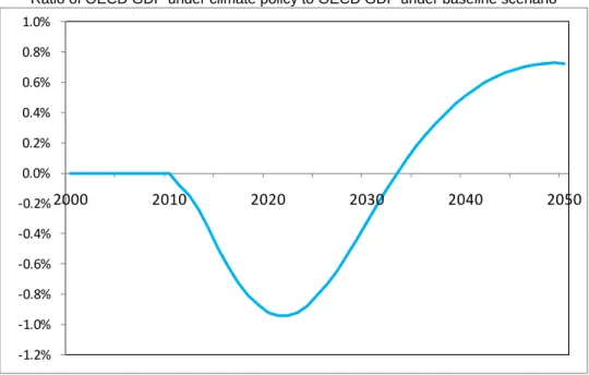
As section 3 aims at evaluating possible impacts of local policies, it is important to bear in mind the impacts that a carbon policy alone might entail without the urban module in the IMACLIM-R model. The results in terms of cost effects of implementing a single carbon tax can be expressed as the ratio of GDP under the carbon tax compared to the baseline scenario (no carbon tax). In the first 20 years of the carbon tax implementation period the OECD economy faces significant, yet temporary, losses with respect to the baseline (in which no tax is put into operation). This is due to the initially strong increase of the price of carbon, which tends to accelerate technical change despite the inertias characterizing the renewal of production equipment, technologies and infrastructure. By 2032, the improvement of energy efficiency confirms to be highly beneficial for the economic activity, especially because it renders the economy less vulnerable to oil shocks. This is captured by a rapid increase in GDP (Figure A.1).

Figure A.1. Economic Impact of a Climate Policy Alone using the Baseline Scenario

Ratio of OECD GDP under climate policy to OECD GDP under baseline scenario

‐1.2% ‐1.0% ‐0.8% ‐0.6% ‐0.4% ‐0.2% 0.0% 0.2% 0.4% 0.6% 0.8% 1.0% 2000 2010 2020 2030 2040 2050

Credits for cover photos (from left to right) are as follows:

Réf. 13649991 © MissMedia - Fotolia.com Réf. 17570634 © shocky - Fotolia.com Réf. 1010731 © Matt Poske - Fotolia.com