Understanding the Reallocation of Displaced Workers to Firms

(1)

HAL Id: halshs-03082302

https://halshs.archives-ouvertes.fr/halshs-03082302

Preprint submitted on 18 Dec 2020

HAL is a multi-disciplinary open access archive for the deposit and dissemination of sci-entific research documents, whether they are pub-lished or not. The documents may come from teaching and research institutions in France or abroad, or from public or private research centers.

L’archive ouverte pluridisciplinaire HAL, est destinée au dépôt et à la diffusion de documents scientifiques de niveau recherche, publiés ou non, émanant des établissements d’enseignement et de recherche français ou étrangers, des laboratoires publics ou privés.

Understanding the Reallocation of Displaced Workers to

Firms

Paul Brandily, Camille Hémet, Clément Malgouyres

To cite this version:

Paul Brandily, Camille Hémet, Clément Malgouyres. Understanding the Reallocation of Displaced Workers to Firms. 2020. �halshs-03082302�

(2)

WORKING PAPER N° 2020 – 82

Understanding the Reallocation of Displaced

Workers to Firms

Paul Brandily Camille Hémet Clément Malgouyres

JEL Codes: J63, J31

(3)

Understanding the Reallocation of Displaced

Workers to Firms

Paul Brandily

*

_{Camille Hémet}

†

_{Clément Malgouyres}

‡

December 15, 2020

Abstract

We investigate the cost of job displacement using administrative data from France that covers employer and employee over both employment and unem-ployment spells. We find that displaced workers experience earnings losses both because of a decline in hours worked (especially in the short run) and because of lower re-employment hourly wages. In line with an active literature, we find that loss in employer-specific wage premium drives most of earnings losses in the long run. However, displaced workers tend to be re-employed by more pro-ductive firms. This result contrasts strikingly with the strong positive correlation between firms’ productivity and wage premium in the cross-section. We further show that the re-employment firms also display lower labor shares. Overall, our results show that the commonly estimated loss in wage premium following job displacement does not reflect a reallocation toward low productivity firms. In-stead they are most consistent with a loss in bargaining power and reallocation towards low-labor share firms.

JEL classification: J63, J31

Keywords: Displaced workers, Wage, Reallocation, Labor share.

*_PSE

†_{PSE, ENS/PSL}

‡_{PSE-Institut des politiques publiques}

We thank participants at the INSEAD - Collège de France brownbag seminar, at the Public Pol-icy Institute (IPP) internal seminar, at the Université Paris-Saclay (RITM) seminar and at the PSE macroeconomic workshop for useful comments. This work is supported by several public grants overseen by the French National Research Agency (ANR): ANR-10-EQPX-17 - Centre d’accès sécurisé aux données - CASD, ANR-18-CE22-0013-01 and the EUR grant ANR-17-EURE-0001.

(4)

1 Introduction

Declining industries and struggling businesses are the inevitable consequences of a changing economy. An economy’s ability to direct resources to productive uses fol-lowing business restructurings has important implications for its aggregate perfor-mance (Foster et al., 2001). In standard models of misallocation (Hsieh and Klenow,

2009), the process of reallocation has clear social benefits but no explicit private cost. Yet, in any economy where factors of production are paid above their cost of oppor-tunity, the reallocation of factors of production from downsizing to expanding firms is likely to be costly for the concerned factor.

This phenomenon is particularly well documented in the case of labor by the liter-ature on job displacement, which has consistently documented substantial long-run losses since the early papers byJacobson et al.(1993) andFarber(1993). Recent contri-bution to this literature go further and shed light on the role of reallocation between firms in explaining such losses. In particular, and even though they point to different magnitudes, several recent studies (Gulyas and Pytka, 2019; Lachowska et al., 2019;

Moore and Scott-Clayton, 2019; Schmieder et al., 2020) find that a substantial part of earnings losses is explained by the loss of firm-specific premium. In these papers, premium are measured as firm fixed-effects retrieved from two-way fixed effects re-gressions following the method ofAbowd et al.(1999) (henceforth AKM). Productivity and wage premium being positively related across firms (Card et al.,2013), the reallo-cation of displaced workers to lower-wage firms appears likely to reflect movements toward lower productivity firms. It could instead be driven by reemployment at low labor share, high productivity firms (Autor et al., 2020). Both possibilities would be compatible with the documented earnings losses but would have different implica-tions regarding the efficiency of labor reallocation in the wake of downsizing event. Yet, little is known regarding the productivity of firms where displaced workers end up being re-employed.

In this paper, we fill this gap by studying the earnings losses following job dis-placement in France and contrasting the features of the sending (firing) and receiving (hiring) firms. Our results are as follows. Looking at a large set of workers dismissed for economic reasons, we first find evidence of large and persistence earnings losses, which still represent more than a third (36%) of pre-displacement earnings after 6 years. Using detailed administrative data on hours worked, we find that while work-ing time explain almost all of the short run losses (1 to 2 years post-displacement), this component of earnings tends to recover in the medium run. By contrast, losses

(5)

in hourly wage rate are smaller in magnitude, but show no sign of recovery within 5 years after displacement. These persistent losses in hourly wage are explained to a very large extent (84.5%) by loss in firm wage premium—which we measure using the standard AKM framework. We find broadly comparable patterns focusing on a sample of mass layoff whose definition follows the standard of the literature.

This first set of results is in line with the long-run earning losses measured in the literature, even though there is no consensus on the role played by firm premium ((Lachowska et al.,2019;Schmieder et al.,2020;Gulyas and Pytka,2019)). Having this in mind, we then go one step further to understand the mechanisms driving this loss in firm premium. Specifically, we show that the reallocation of workers to lower wage premium firms does not reflect a reallocation towards low productivity firms. Instead we find that displaced workers are disproportionately hired by high productivity firms which display a lower wage premium and a lower labor share of value-added. While among the cross-section of firms, higher productivity is associated with higher premium, hiring firms tend to be both more productive and paying lower premium than firing firms. Comparing firing and hiring firms to the rest of active firms in the economy, we show these firms to be more productive and paying higher wage premium than the average firm in the economy. Overall, this pattern suggests that the private losses experienced through lower wage premium is more likely to represent a decline in bargaining power than a reallocation toward less productive firms. As such, it could suggest that the social cost of job displacement does not exceed its private cost.1

We contribute to the literature in two main ways. First, thanks to an administra-tive definition of lay-off for economic reasons, we are able to focus on a larger set of involuntary labor market separations for economic reasons, as opposed to dismissal for cause, than what is captured by the reliance on mass lay-off episodes associated with a specific share decline of firm (or plant) level employment—typically in ex-cess of -30% (Jacobson et al., 1993; Kletzer, 1998). We show however that our results are robust to using a sample of workers displaced from mass-layoffs comparable to the rest of the literature. Second, we document precisely the components explaining

1_{Naturally, establishing this would require measuring the marginal productivity of displaced workers}

in their new workplace which is not feasible with the data at hands. However given that losses in firm-wide wage premium account for a large fraction of losses in hourly wage rate, individual specific decline in productivity, such as depreciation in human capital (Burdett et al.,n.d.) or losses in worker-firm matches (Lachowska et al.,2020), does not appear to be of first order importance in our setting. At any rate, we show that workers are reallocated to work places where average labor productivity is high.

(6)

earnings losses in hours and hourly wages, and the fraction of the hourly wage that is explained by loss in firm-specific wage premium. Although these decomposition exercises were performed in previous studies, we go one step further by digging into the underlying channels for losses in wage premium. Specifically, we contrast these losses in wage premium with other features of the receiving employers, focusing on measure of productivity, available surplus per worker (value-added per worker) and labor compensation as a percentage of overall value added. Doing so, we observe that displaced workers tend to reallocate toward more productive firms, suggesting that the overall effect is driven by a reduction of their bargaining power.

The remainder of the paper is as follows. Section2provides a detailed description of the data we use and of the institutional context. Section 3 presents our empirical approach and our main results regarding the earnings loss due to job displacement and the role of losses in firm specific premium in shaping overall job displacement effects. Section4studies the productivity and performance of the firms where workers end up being re-employed. It further studies the correlates of wage premium and compare the characteristics the firing and hiring firms in our sample with respect to the rest of the corporate sector. Section 5concludes.

2 Data

We rely on French administrative data sources to identify and follow the trajectories of workers affected by a displacement. We complement this analysis with firm-level administrative data sources. In this section we first present the French institutional context that enables us to identify workers laid-off for economic reason 2.1. We then present the main data sources used to build our sample and to measure firm charac-teristics in subsection2.2. Finally, subsection2.3 briefly describes our main sample of analysis.

2.1 Displaced workers

2.1.1 Institutional background: economic layoffs in France

In France, as in most OECD countries, separations and dismissals are classified into different types, depending on whether they are justified on economic or personal or

(7)

disciplinary grounds. Given the scope of this paper, we focus on a panel of workers administratively registered as "laid-off for economic reasons" (licenciement économique, LE henceforth) at the French employment agency, between 2002 and 2012. We ar-gue that focusing on these LE workers has three main advantages. First, it allows us to minimize the risk studying individuals who voluntarily left their firm and whose employment trajectory is highly endogenous. Indeed, this administrative status of laid-off for economic reason is defined by law and characterizes separations that are most likely caused by poor economic performances. Second, relying on this sample does not require us to select specific firms, contrary to what is done in the literature on mass layoffs. Finally, we note that by using such administrative definition we en-sure that all LE individuals face similar unemployment insurance scheme. We now detail further the first two advantages.

Our first point directly follows from the legal definition of LE. In France, in or-der to displace workers for economic reasons, the employer has to provide evidence of the existence of economic difficulties for the firm. Under French law, “economic reasons” entail mainly four types of situations: (i) “difficulties” (persistent reduc-tion of turnover, reducreduc-tion of gross income, etc.), (ii) “technological transformareduc-tion” (implying the need for different skills), (iii) “re-organisation” (in order to anticipate type-(i) issues, as opposed to improving performance) and (iv) “cessation of busi-ness”. Economic dismissal can be individual or collective. During collective economic lays-off, the employer must also justify its choice of who remains employed and who is laid-off. As pointed out byBatut and Maurin(2020), French labor laws suggest em-ployers to dismiss lower seniority workers first, as well as workers with lower family responsibility (see article 1233-5 of French labor laws). The process for “licenciement économique” depends on the size of the firm and the number of affected workers, with more stringent conditions regarding retraining imposed upon larger employer (Bender et al.,2002).2 Considering the very strict legal definition and associated condi-tions, it is therefore unlikely that a firm could misclassify a layoff for personal reason as an economic layoff. Yet, because dismissals for personal reasons are more likely to be contested in court than economic layoffs (Fraisse et al., 2015), one may suspect some employers to disguise personal dismissals as being economic in order to avoid

2_{France being characterized by a high level of employee protection legislation (EPL) – in particular}

for permanent contracts (OECD,2004) – terminating a contract (as LE or another type of layoff) has economic consequences not only for the worker but also for the firm. For instance, laying-off workers for economic reasons imply severance payments.

(8)

litigation costs. However, Signoretto and Valentin(2019) provides an empirical analy-sis of the firm-level determinants of this choice (economic versus personal) and finds that economic dismissals are overwhelmingly explained by the economic conditions of firms (whereas personal layoffs are predicted by other variables – such as the propen-sity of human resource management to retain employees). Overall, this suggests that economic dismissals are primarily driven by economic circumstances experienced by the firm and not by individual factors. As such, LE provide a shock to individual workers that is unlikely to be the result of his own will. It is also worth stressing that because our sample is based on the reason for the layoff as legally reported, it reflects the employer motivation for the layoff rather then workers’ subjective perception of the ultimate cause for the dismissal.

The second advantage of working on a sample of LE workers is to enable us to rely on a more representative set of employers, especially compared to the literature focusing on mass-layoffs. Many studies in the displaced workers literature use panel data on workers to identify events that can be suspected of being a mass layoff (e.g.

Jacobson et al.,1993; Gathmann et al.,2020;Gulyas and Pytka,2019;Lachowska et al.,

2019;Schmieder et al.,2020). The typical definition of a mass layoff event is an episode over one or several years where firms see their employment decline by more than 30 percent. This approach is often justified in part because the administrative data do not distinguish directly between quits (voluntary separations) and layoffs (involun-tary separations).3 In effect, it requires the researchers to assume that all separations from firms experiencing a mass layoff are involuntary. Perhaps more importantly, this approach implies that the analysis focuses on a minority of displaced workers, in particular because the mass layoff studies often impose some restrictions on the size of the employer (so that the 30% decline would not simply reflect some small number variability)4 as well as on the tenure of workers. The tenure requirements imply that the focus of such studies is on workers for whom the employment rela-tionship was most valuable (Kletzer,1998)—thus resulting in a potential upper bound on the effect of displacement. The focus on fairly large firms, which are more likely to provide more general training, might on the other hand result in a lower bound of the average displacement cost—especially if some separations are voluntary. Relying

3_{This is the initial concern of} _{Jacobson et al.} ₍₁₉₉₃_{), that actually observe separations but not their}

cause.

4_{For instance,}_{Schmieder et al.} ₍₂₀₂₀_{) focus on employers with at least 50 employees which is typical}

(9)

on the administrative definition of economic layoffs enables us to avoid these caveats. Nonetheless, with the data at hand, we also build a second sample of mass-layoffs (the “MLO sample”) following the approach adopted in the above-mentioned papers. We use this second sample to analyze specific aspects of the layoffs, but also to confirm our main analysis and compare it more directly with the rest of the literature. An important difference between LE and MLO individuals is that the LE do need to tran-sit by unemployment insurance, while MLO workers may find a job without needing any unemployment benefit—especially if a fraction of MLO sample separations are voluntary.

2.1.2 Data

Our main sample consists in a panel of LE workers, for whom we can not only char-acterize the unemployment spell following the economic layoff, but also the employ-ment history before and after this event. Being able to track these individuals over time and across employment statuses is made possible by using the FH-DADS data, a unique panel resulting from the merge of two administrative datasets thus cover-ing both employment (DADS) and unemployment (FH) episodes. More precisely, the DADS (Déclaration Annuelle des Données Sociales) is a matched employer-employee dataset nearly covering the universe of employees in the private sector in France over the 2002-2012 period. This DADS comes from the administrative declaration that all employers report annually to social security authorities and tax administration, whereby they provide information on both their establishments (e.g. size, industry and municipality) and on each employee (occupation, wage, hours worked, start and end date, type of contract, etc.).

The panel version of this dataset which allows us to follow workers over time contains 1/12 of the universe of jobs. This panel is matched to the FH (Fichier His-torique) data, an historical administrative file produced by the national unemploy-ment agency (Pôle Emploi) which records individuals’ unemployunemploy-ment spells. Any em-ployment seeker who wishes to claim unemem-ployment benefits must register to Pôle Emploi, and therefore appears in the FH. The FH contains information about date of registration, duration and amount of unemployment benefits, etc. Crucially, this dataset enables us to precisely identify LE workers (laid-off for economic reasons) as it documents the administrative reason (or “cause”) for registration. In addition, we observe some dimensions of the job search and, in particular, reservation wage, on

(10)

which we intend to rely to document job search behaviour.5

2.1.3 Sample construction

Workers laid-off for economic reasons (LE panel). To construct the LE panel, we need to link a specific LE-registration (in the FH) to a specific job (in the DADS), which is not clearly identified. We define a laid-off worker’s previous job as the position which end date is the closest to the end of contract date recorded by the unemployment agency. In line with the literature, we are interested in individuals losing their main, stable job. We therefore select workers based on the following rules: they must be aged between 25 and 60 in the year they register as LE (year t); they must have worked more than 1800 hours in the previous job in years t−1 and t−2; and we also make sure they are not employed in the same firm on June 30, t+1. A given individual is included in the sample only when he is first registered as LE and complies to the aforementioned selection rules.6

We provide descriptive statistics for the LE sample in tables1 and 2 as well as in Figure1 below. We comment these statistics more thoroughly in the next subsection. In total, 2 semesters before their layoffs we observe 16,434 LE individuals, displaced in 13,463 events (i.e. firm times year layoffs).

Control group. We use propensity score matching to construct a control group for the LE workers. We perform the matching on all workers found in DADS (excluding those belonging to the LE panel) and who meet the basic criteria also applied to the displaced workers, namely: the individual must be between 25 and 60 in year t; he must have worked more than 1800 hours in the same job in years t−1 and t−2. We then perform the matching within year and sector (2 digits-level, 99 sectors) using the following variables: age in t, plant size in t−1, hourly wage in t−1 and t−2, number

5_{To be more specific, workers fill in their reservation wage once, at registration, in order to help the}

agency to select appropriate job offers.Barbanchon et al.(2019) provide more details on the reservation wage and confirms the quality of the measure. For instance, they show that higher minimum wage are associated with higher unemployment spells once accounting for individual fixed-effects. In the version of the dataset they use however they do not dispose of reemployment wages, and accordingly cannot assess directly the link between reservation and reemployment wages.

6_{That is to say: (i) we ignore LE from a job that does not meet the criteria (i.e. part-time, low tenured,}

(11)

of hours worked in t−1 and t−2.7 We keep the nearest neighbor, with replacement, using a simple probit model.

Workers displaced during mass layoffs (MLO panel) As mentioned before in sec-tion 2.1.2, we build a second sample made of individuals working in closing plants that we qualify as mass-layoffs, closer to what the literature usually uses. We describe the construction of this sample as well as its summary statistics in appendixC.1.

In summary, this sample is made of any worker who was a full-time employee (in t−2 and t−1) of a plant that closed in year t, where we define closure as a reduction of employment of 90% or more. We purposely choose a very high threshold as compared to the literature (where it usually is 30%) because we want to rely on individuals who are very unlikely selected within the workplace (i.e. workers whose dismissal is orthogonal to their characteristics). Our MLO panel includes 12,815 such workers, displaced from 6,617 events (i.e. firm times year layoffs). We eventually match these MLO individuals to a control group built in the same spirit as for the LE sample.

2.2 Firm characteristics

In order to understand the losses associated to economic layoffs, we use two ad-ditional sources of data to characterize pre-layoff firms (to which we alternatively refer as sending or firing firms) and post-layoff firms (called receiving or hiring firms henceforth).

2.2.1 Data

Firm premium. We compute firm premium relying on the exhaustive version of the DADS (so-called “DADS postes”), which covers the universe of workers employed in France over the 2001-2014 period. Each firm is identified with a unique administrative number (the 9 digit SIREN code) that remains constant across years. It allows match-ing each employee to an employer and trackmatch-ing firms’ employment and wage policy over time. This dataset does not allow us to build a panel of workers because each

7_{Here, we refer to wages and hours from the main job. In further analysis, we sometime include (and}

(12)

worker is assigned a new identifier at each vintage. We can however track individu-als across jobs within a given year t as well as between year t and t−1, because any vintage t of DADS-postes contains information on jobs existing at time t and t−1.8

This data allows us to compute firm premiums for a large group of employers. Since the exhaustive DADS is a panel at the firm level but only a rolling window (yearly) panel at the individual level, it is possible to estimate an AKM model on this data, but not to map the individual fixed effect from this version of the DADS to the panel version we use to build our main sample (LE sample). In summary, using the exhaustive version of DADS allows us to estimate firm fixed-effects for a larger set of firms compared to studies focusing on the worker-level panel, but this comes at the cost of not being able to retrieve worker fixed-effects and use them with the worker-level panel.

Other firm characteristics. We also build measures of labor productivity and the labor share using income statement and balance-sheet data coming from the FICUS database. FICUS is a nearly exhaustive administrative dataset covering the universe of firms in the private sector, at the notable exception of the agricultural and the financial corporate sectors. FICUS is built from the tax returns of firms and their social security declarations. It provides detailed information on firms’ revenues and expenses.

2.2.2 Firm premium

We compute firm premium in a standard AKM framework for three periods of 4 to 5 years (2001-2004, 2005-2009, 2010-2014), using the exhaustive version of the DADS. For each period, we estimate the following model:

ln(wit) = ψJ(i,t)+αi+λt+x0itβ+eit (1)

where ψ_J(i,t) is the firm fixed effect associated with the firm J(i, t) where worker i was employed at period t. αi is an individual fixed effect and λt a set of time fixed

effects. Time varying controls are included in the vector xit. Finally, the dependent

variable wit refers to worker i’s hourly wage in year t. Further details on the

imple-mentation of the two-way fixed effects estimation with the exhaustive version of the

8_{Note that the individual-level unique identifier from the exhaustive version of the DADS presented}

here and the panel version of the DADS presented in section 2.1.2 are different, so that we cannot merge the exhaustive and panel datasets at the worker-level.

(13)

dataset is provided in section B of the appendix. In our main analysis, we rely on fixed effects estimated over the 2001 to 2004 period, i.e. before the layoffs we focus on. That way, we characterize and "compare" firing and hiring firms in a period that is sufficiently early before the event to avoid these characteristics being affected by the layoffs (e.g. firing firms’ characteristics tend to vary within two years preceding the layoffs, while hiring firms are "survivors" whose characteristics may differ after other firms closed or went through financial difficulties).

2.2.3 Other firm characteristics

In order to investigate further the relative characteristics of sending (firing) versus receiving (hiring) firms, and to understand the dynamics underlying the reallocation process, we measure additional firm characteristics using FICUS data. In particular, we build two measures of labor productivity: our first direct measure is the value added per worker, while our second measure accounts for differences in capital in-tensity. More precisely, this alternative measure of productivity is the residual of a regression of value-added onto tangible and intangible capital and employment. Moreover, we also compute firms’ labor share as the ratio of total labor costs over the value added.

Importantly, our main analysis also relies on measures taken over the period pre-ceding the layoffs under study (2001-2004), for the sake of consistency with the period over which firms fixed effect are estimated. Alternatively, we compute the average of firm characteristics over a three-year period, centered around five years before dis-placement (t−5). That is, for a worker laid-off in 2011, we measure the characteristics of the firm that fired him and of the firms where he is re-employed as the 2005 to 2007 averages of the variables at hand. These rolling-window measures of firms’ characteristics are currently used to test the robustness of our results in section 4.

2.3 Descriptive statistics on the estimating sample

Our main sample (the LE sample) consists of 32,868 individuals equally distributed among treated and control individuals. Table 1 reports the mean and standard de-viation of the six quantitative variables measured at baseline and used to match dis-placed individuals to suitable controls (cf. above). The average disdis-placed individuals is almost 45 years old, works in a firm employing 553 employees and earned 17.53 (respectively 17.43) euros per hour in year t−1 (t−2), over which he worked 1,917

(14)

hours (respectively 1,917). Given the matching procedure described above, it comes at no surprise that these variables are well balanced across groups. In column (3) we report the Imbens & Rubin “normalized difference” (a scale-free measure used to compare two distributions). Imbens and Rubin(2015) suggest that this value should never exceed 0.25, which is always the case here.

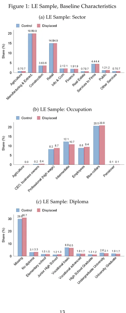
Table 2 and Figure 1 report the distribution of quantitative and qualitative vari-ables, respectively, that were not directly used in the matching process. In these dimensions as well, both treated and control groups look similar. Table 2 shows that about two thirds of the sample are males, who earned about 35,500 euros in t−1 when considering all their contracts, that is when taking into account that (beyond their main job) they worked in about 1.05 firms on average. Finally, we also verify that the two groups were, on average, employed in similar type of firms, as measured by the pre-layoff firm wage premium – estimated from the AKM framework using exhaustive data of firms over the 2001-2004 period (as explained in subsection 2.2.2). Here again, none of the differences in distribution seems to exceed Rubin and Im-bens rule of thumb. Figure 1 finally displays the distribution of treated and control individuals by categories of sector of employment (1a), occupation (1b) and highest diploma (1c). The distribution across sector is balanced by construction; while the bal-ance in the two other qualitative variables can be seen as a test of the procedure. One year before layoff, displaced and control workers mainly worked in manufacturing and extraction or the retail sectors; a large share were blue collars, clerical (called “in-termediate professions” in the French classification) or employees. The information about diploma is missing for a large part of the sample (and we most often exclude it from further analysis) but the balance among observed individual remains (with the highest observed share being vocational basic training).

(15)

Figure 1: LE Sample, Baseline Characteristics (a) LE Sample: Sector

(b) LE Sample: Occupation

(16)

Table 1: Matching variables

(1) (2) (3)

LE Control Norm. Diff.

Age 44.83 45.05 -0.02 (9.85) (9.45) (0.00) Wage rate t₀D−1 17.53 17.88 -0.02 (10.69) (10.26) (0.00) Wage rate t₀D−2 17.43 17.74 -0.02 (10.61) (10.25) (0.00) Hours worked tD₀ −1 1917.29 1920.79 -0.02 (132.19) (139.36) (0.00) Hours worked tD₀ −2 1917.18 1920.40 -0.02 (130.55) (139.25) (0.00) # employees at firm t₀D−1 553.35 516.07 0.02 (1829.89) (1554.01) (0.00) Obs 16434 16434 32868 Events 13463

Notes: Individuals are observed 2 semesters before layoff. Here, events are defined as all layoffs taking place in the same firm, commuting zone and year The last column reports Imbens-Rubin, Normalized difference.

Table 2: Matched samples

(1) (2) (3)

LE Control Norm. Diff.

Gender: Male 0.65 0.68 -0.04 (0.48) (0.47) (0.00) Gross earnings 35513.22 36140.81 -0.01 (34408.27) (32509.70) (0.00) # of employers 1.05 1.05 0.01 (0.34) (0.45) (0.00) Firm-wage premium 01-04: bψJ(i,t) 0.09 0.07 0.04

(0.37) (0.20) (0.00)

Obs 16434 16434 32868

Events 13463

Notes: Individuals are observed 2 semesters before layoff. Here, events are defined as all layoffs taking place in the same firm, commuting zone and year The last column reports Imbens-Rubin, Normalized difference. bψ_J(i,t)refers to AKM firm-fixed effects, see Section2.2.2for details on their estimations.

(17)

3 Earning loss and the role of firm premium

In this section, we show evidence that past-employer wage premium contributes to post-displacement long-term losses in a sizeable way. To do so, we first follow the ex-isting literature and analyze the long-term losses of displacement in France in subsec-tion3.1. We then assess the importance of past-employer wage premium in explaining loss differences in subsection3.2.

3.1 Average displacement effects

We estimate long-term displacement losses using the following standard model:

Yit = 5

∑

d=−2 βd×1{tDi +d =t} ×1{Di =1} + 5

∑

d=−2 δd×1{tDi +d=t} +αi+δt+ei (2)

Where Yit is an outcome of interest measured in year t for individual i, who was

displaced in year tD_i . The coefficient βdmeasures the change in Y for displaced

work-ers (indicated by D =1) compared to the control group counterfactual, d periods after displacement. The model includes worker (αi) and year (δt) fixed-effects. Standard

errors are clustered at the individual level.9

We start by estimating equation 2 alternatively using overall earnings and em-ployment status as outcomes. Figure 2reports the losses induced by displacement in terms of annual earnings. The magnitude of the losses culminates 1 year following displacement (t+1) at about e19,500, which represents roughly 55% of the baseline annual earnings (see Table 2). The losses attenuate over time and represent slightly more than e13,000 at t+5, i.e. about 36% of the baseline earnings.

9_{Note that we use a matching procedure with replacement. This implies that some non-displaced}

individuals may enter the control group multiple times if they are the best match for several displaced workers. In this case they will appear under different “worker” identities. We cluster standard errors at the true “individual” level however to account for the dependence between observations that this may introduce.

(18)

Figure 2: Displacement Effects: Annual Earnings -20000 -15000 -10000 -5000 0 -2 -1 0 1 2 3 4 5 6

Time relative to displacement

Notes: The sample contains 16434 economic dismissals. 99% confidence interval are displayed, based on robust standard errors clustered at the worker-level. The specification includes individual and year fixed-effects, see equation (2) and associated text for more details.

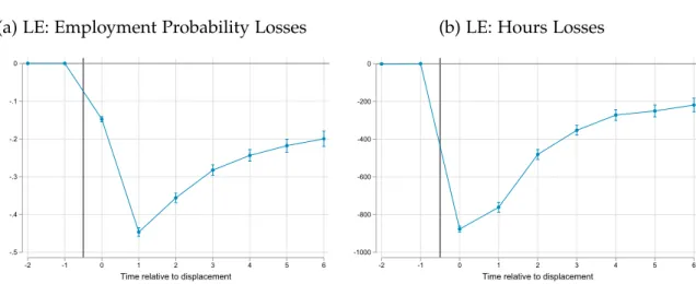
This decline in annual earnings is driven both by a decline in employment and in the number of hours worked, and by a reduction in hourly wage. The drop in employment is depicted in Figure3a: immediately after the event (t+1), the employ-ment probability of displaced workers is about 44 percentage points lower than that of the control group. This effect progressively attenuates overtime, up to reaching -20 percentage points after 6 years. On top of this extensive margin effect, we observe an effect at the intensive margin as well: Figure 3b reports the effect on the number of hours worked, focusing on re-employed workers only. The drop in the number of hours reaches its lowest at t, at slightly less than 900 hours, and tends to recover with time: 6 years after the event, we still observe a loss in the number of hours worked of around 220 hours. Combined together, these findings suggest that in the medium run, both margin contribute to reducing the overall loss in hours worked.

(19)

Figure 3: Displacement Effects: Employment at the intensive and extensive margin (a) LE: Employment Probability Losses

-.5 -.4 -.3 -.2 -.1 0 -2 -1 0 1 2 3 4 5 6

(b) LE: Hours Losses

-1000 -800 -600 -400 -200 0 -2 -1 0 1 2 3 4 5 6

Notes: The sample contains 16,434 economic dismissals in panel (a), and 11,117 events in panel (b) which focuses on re-employed workers only. 99% confidence interval are displayed, based on robust standard errors clustered at the worker-level. The specification includes individual and year fixed-effects, see equation (2) and associated text for more details.

We then repeat the analysis using the hourly wage rate as the dependent variable, where the wage rate is only defined for those workers who have been re-employed after layoff, so that the composition of the sample is actually changing over time. Specifically, as the length of time post-displacement increases, so does the average number of workers back to employment, as illustrated in Figure 3a. The sign of the bias induced by such composition changes is not clear. For instance, to the extent that intrinsically low-wage workers take longer to regain employment, and do so at lower wages, the persistence in the loss in terms of hourly wage could be overestimated. Nevertheless, the overall impact of hourly wage could be underestimated, if high-wage workers are more likely to remain in the estimating sample at any point in time.

The change in (log) hourly wage, depicted in Figure 4, displays a noisy (yet fa-miliar) pattern at year t. This is arguably driven by some measurement error or selection of very specific workers who quickly re-enter employment. Another expla-nation for this pattern lies in the fact that severance payments are included in earnings in our data, hence artificially increasing hourly wage at the time of layoff. Interest-ingly, while the pattern of losses in overall earnings, employment, and hours worked showed a clear recovery, we see that the loss in log hourly wages tends to stagnate in the medium run at around -0.12. This finding is in line with recent research on displacement in other countries or over different periods, such as in Lachowska et al.

(20)

Figure 4: Displacement Effects on (log) Hourly Wage Rate -.15 -.1 -.05 0 .05 .1 -2 -1 0 1 2 3 4 5 6

Notes: The sample contains 11,117 economic dismissals. 99% confidence interval are displayed, based on robust standard errors clustered at the worker-level. The specification includes individual and year fixed-effects, see equation (2) and associated text for more details.

3.2 The role of employer wage premium in shaping earnings losses

A key question to understand the reduction in earnings associated with job displace-ment is to assess whether it is driven by a deterioration of the quality of jobs to which displaced workers have access. Early papers defined job quality based on industry-wide premium and tended to find that displaced workers experienced wage losses through the loss of wage industry fixed-effects (Krueger and Summers,1988). Extend-ing this literature, more recent papers have used matched-employer employee data and the AKM framework to show that inter-industry wage differentials are mostly the reflection of pervasive and persistent firm-level wage differentials (Goux and Maurin,

1999; Card et al., 2013; Song et al.,2019).

Whether the loss of firm-level wage premium (as proxied by firm fixed-effects estimated in the AKM framework) represents a sizable contribution to the earnings losses of displaced workers is a topic of active research. Recent papers byGulyas and Pytka(2019) andSchmieder et al.(2020) find that firm premium play an important role in shaping earnings losses, consistent with the work of Goldschmidt and Schmieder

(2017) on outsourced workers. Conversely,Lachowska et al.(2020) find this source of loss to be of modest quantitative importance.

(21)

the loss in firm-specific wage premium in our context. To do so, we use firm premium as a dependent variable in our main model (equation 2). In Figure 5, we represent the associated coefficients. For the sake of comparison, Figure 5 also reports the co-efficients associated to estimations with our previous three main dependent variables (total earnings, hours and hourly wage, all taken in log). Because we want to compare our results to the literature, we also reproduce the same analysis using our MLO sam-ple and present the results in Figure6. An important difference between our analysis on economic layoffs and the mass layoff literature is that a LE requires individuals to register into unemployment; while mass layoffs also include individuals who imme-diately find a job after displacement, which contributes to explain why the losses are of a lower for the MLO sample. An additional advantage of the MLO sample is that it spans over a longer time period, allowing us to look at additional pre-layoffs periods and hence assess the absence of pre-trends.

To give a sense of the contribution of firm premia in explaining the loss in hourly wages, Lachowska et al. (2020) report the loss in log premium at t+5 (they find -0.020) to the total loss in log hourly wage at t+5 (-0.115) whereby they obtain that firm premium loss explains 17 percent of the total loss in hourly wage at t+5.10 We repeat this exercise on our two samples and find that loss in premia explains 84.5% (-0.093/-0.11) of hourly wage loss in the LE sample and 95.5% (-0.063/-0.066) in the MLO sample at t+5. In other words, although our estimates of total hourly wage loss at t+5 are roughly comparable (around 10%), we find evidence that the loss in firm premium contributes to a much greater extent to hourly wage loss in our context. As we also happen to find much larger earning loss thanLachowska et al.(2020), the contribution of premium loss to earning loss at t+5 that we obtain for the LE sample (22.3%) is closer to theirs (12%).1112 Our findings are actually closer to Schmieder et al. (2020) where the contribution of firm premia to hourly wage losses are around 76%.13 Schmieder et al. (2020) also provide two useful observations: first, although

10_{These comparisons are built from}_{Lachowska et al.}₍₂₀₂₀_{), Table 2.}

11_{However, the contribution of premium loss to earning loss at t}₊_{5 that we obtain for the MLO sample}

is larger, at 37.5%.

12_{Note also that we find much stronger (log) total earnings and hours effect than} _{Lachowska et al.}

(2020). At t+5, log earnings in the LE sample (respectively, MLO) decrease by -0.417 (-0.160) and log hours by -0.307 (-0.094) as compared to -0.164 and -0.047 inLachowska et al.(2020). The discrepancy between our two (LE and MLO) samples show that part of the difference between the two studies is driven by the sample definition.

13_{Cf. Table 3 of (}_{Schmieder et al.}_, ₂₀₂₀_{) that provides losses in log daily wage and firm premium,}

across two different moment of the business cycle. Estimate in recessions in 76.3% (6.94/9.09) and 75.5% (3.91/5.16) in booms.

(22)

wage losses differ between booms and recessions, the total contribution of firm premia seems stable along the business cycle; second, they discuss the potential causes of the different estimations of the premium contribution, attributing at least part of the gap to composition effects (i.e. different distribution of observed displaced workers across type of firms). We conclude from this analysis that firm premium loss is an important contribution to hourly wage loss. In our specific case, because we observe that loss in premium accounts for most of the loss in hourly wage, we argue that firm-premium loss matters more than alternative explanations such as employer-employee match effects.14

Figure 5: Loss in wage premium: Economic layoffs (LE) sample

-1 -.75 -.5 -.25 0 .25 -2 -1 0 1 2 3 4 5 6

Premium Log Hourly wage Log Hours Log Earnings

Notes: 99% confidence interval are displayed, based on robust standard errors clustered at the worker-level. The specification includes individual and year fixed-effects, see equation (2) and associated text for more details.

(23)

Figure 6: Loss in wage premium: Mass-layoff (MLO) sample -1 -.75 -.5 -.25 0 .25 -5 -4 -3 -2 -1 0 1 2 3 4 5 6 7 8

Premium Log Hourly wage Log Hours Log Earnings

Notes: 99% confidence interval are displayed, based on robust standard errors clustered at the worker-level. The specification includes individual and year fixed-effects, see equation (2) and associated text for more details. Details on the contruction of the sample are provided in AppendixC.1.

A question naturally follows from this conclusion: are these losses in firm pre-mium due to workers reallocating in low-productivity, low-wage firms? Or are they driven by a loss in bargaining power (with for instance, the reallocation to low-wage, high-productivity firms)? While the first case implies that the reallocation process is likely to be inefficient; in the second case, this process would mostly entail redistribu-tive consequences with lower losses in potential output.

4 The reallocation of displaced workers across firms.

In the previous section, we established that displaced workers are reallocated to low-wage premium firms, low-wage premium being estimated over the 2001-2004 period for all firms (Figure5). A natural explanation of this result could be that displaced workers are reallocated towards low-productivity firms, which tend to pay lower-premium. Indeed, as we document just below in section 4.1, more productive firms tend to pay higher wage premium. However, we show in section 4.2 that displaced workers are rather re-employed in more productive firms, which nonetheless tend to have a lower labor share of value-added. Eventually, we further explore firms characteristics in section 4.3, comparing firms that fired or hired our displaced workers to other firms.

(24)

4.1 More productive firms, higher wage premium

In Table 3, we present the result of a simple linear regression, where we regress firm fixed-effects from an AKM framework (section 2.2.2) onto a set of accounting vari-ables. Productivity (either directly measured as value-added per worker or through the residual from a regression of value-added on inputs) is among the strongest pre-dictors of firm-wage premium, even after controlling for firm size and sector fixed effects. The unconditional coefficient of correlation between wage premium and ei-ther measure of productivity is about 0.20 (not displayed in the Table). Column (5) and (6) show that older and manufacturing firms, respectively, display a positive wage premium.

Table 3: Firm-level correlates of firm wage premium

(1) (2) (3) (4) (5) (6) (7) (8) Employees 0.0618*** 0.0634*** 0.0571*** 0.0580*** 0.0477*** (96.53) (99.64) (89.29) (87.74) (70.16) VA 0.0751*** (129.91) VA per worker 0.118*** (82.67) Productivity 0.131*** 0.132*** 0.0902*** (89.23) (89.42) (57.19) Age>10 years 0.0395*** -0.00877***-0.00861*** (24.63) (-5.44) (-5.35) Manufacturing 0.0156*** -0.00169 (7.74) (-0.85) Sector FE √ Observations 506036 506036 506036 506036 506036 506036 506036 506036 R2 0.015 0.029 0.032 0.035 0.001 0.000 0.035 0.048 Adjusted R2 0.015 0.029 0.032 0.035 0.001 0.000 0.035 0.048

Notes: t-stat based on robust standard errors in parentheses, clustered at the employer-level. All accounting ratio are in log. * p<0.05, ** p<0.01, *** p<0.001

The positive relationship between value-added per worker is close to what is found inCard et al. (2018) in the case of Portugal. This result is also consistent with the re-sults ofCoudin et al.(2019) who estimate gender specific wage premia and correlation between the estimated premia and value-added per worker as well as with the results ofAbowd et al.(1999)—who regress value added per worker on firm fixed effect.

(25)

4.2 Pattern of reallocation of displaced workers in terms of

firm-productivity.

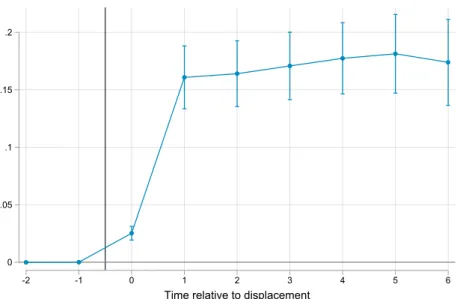
In Figure 7, we show the impact of displacement on the average productivity (ad-justed for capital intensity) of the subsequent employers. As explained in section2.2.3, firm-level productivity is measured over the 2001-2004 period, so that the event study coefficients simply trace out the effect of displacement on the reallocation of work-ers toward differently productive firms. It clearly appears that on average displaced workers reallocate toward much more productive firms than their counterfactual.

Figure 7: Productivity 0 .05 .1 .15 .2 -2 -1 0 1 2 3 4 5 6

Notes: The sample contains 9,251 economic dismissals. 99% confidence interval are displayed, based on robust standard errors clustered at the worker-level. The specification includes individual and year fixed-effects, see equation (2) and associated text for more details. Productivity is computed as the residual of a regression of value-added onto tangible and intangible capital and employment during the period 2001-2004.

The same qualitative conclusion can be drawn from the patterns observed when using value added per worker as an outcome (see Figure 8a). As expected given the average loss in firm premium, we further find that displaced workers also reallocate toward firms with lower labor share of value-added, which is computed as the in-verse of pre-tax value added over reported total labor cost (Figure8b). To get a better sense of the type of firm towards which displaced workers are reallocated, we further look at firm’s size (log of labor force). The pattern displayed in Figure 9 reveals that workers laid-off for economic reasons are re-employed by larger firms.

(26)

Figure 8: Value-added per worker and labor share of value-added (a) Log of value-added per worker

-.05 0 .05 .1 .15 -2 -1 0 1 2 3 4 5 6

(b) Log of labor share of value-added

-.2 -.15 -.1 -.05 0 -2 -1 0 1 2 3 4 5 6

Notes: The sample contains 10,336 economic dismissals. 99% confidence interval are displayed, based on robust standard errors clustered at the worker-level. The specification includes individual and year fixed-effects, see equation (2) and associated text for more details. value added per worker is computed as pre-tax value added over reported employment during the period 2001-2004. The labor share is computed as the inverse of pre-tax value added over reported total labor cost during the period 2001-2004.

Figure 9: Firm size (log of labor force)

0 .5 1 1.5

-2 -1 0 1 2 3 4 5 6

Notes: The sample contains 10,336 economic dismissals. 99% confidence interval are displayed, based on robust standard errors clustered at the worker-level. The specification includes individual and year fixed-effects, see equation (2) and associated text for more details. Productivity is computed as the residual of a regression of value-added onto tangible and intangible capital and employment during the period 2001-2004.

We find that the same reallocation towards high-productivity, low-labor share, large firms applies to the MLO sample as shown in Figure10: workers displaced fol-lowing a mass layoff tend to be re-employed in more productive firms (Figure 10a),

(27)

featuring a larger value-added per worker (Figure 10b), but where the labor share of value-added is nonetheless lower (Figure 10c). Consistent with prior results, MLO workers are also re-employed in larger firms (Figure10d).

We eventually confirm these patterns when computing the average of each firm characteristics (productivity, value-added per worker, and labor share of value-added) over the t−6 to t−4 period, rather than at a fixed point in time (2001-2004). The cor-responding "rolling-window" results are reported in appendixA.2for the LE (Figures

A3and A4respectively).

Figure 10: Productivity, value-added per worker and labor share (MLO sample) (a) Productivity 0 .05 .1 .15 .2 .25 -2 -1 0 1 2 3 4 5 6 7 8

(b) Log of value-added per worker

0 .05 .1 .15 .2 .25 -2 -1 0 1 2 3 4 5 6 7 8

(c) Log of labor share of value-added

-.2 -.15 -.1 -.05 0 -2 -1 0 1 2 3 4 5 6 7 8

(d) Firm size (log of labor force)

0 .2 .4 .6 .8 1 -2 -1 0 1 2 3 4 5 6 7 8

Notes: The sample contains 5,614 mass-layoffs in plot (a); 6,423 in plots (b), (c) and (d). 99% confidence interval are displayed, based on robust standard errors clustered at the worker-level. The specification includes individual and year fixed-effects, see equation (2) and associated text for more details. Produc-tivity is computed as the residual of a regression of value-added onto tangible and intangible capital and employment during the period 2001-2004. Value added per worker is computed as pre-tax value added over reported employment during the period 2001-2004. The labor share is computed as the inverse of pre-tax value added over reported total labor cost during the period 2001-2004.

(28)

4.3 Characterizing hiring and firing firms.

The firms that are laying off workers on economic grounds appears to be different from the firms where these workers are re-employed. This appears at first unsurpris-ing: shrinking firms are expected to be less dynamic than expanding ones, almost by definition. The interesting pattern however is that while the firing firms tend to be less productive than those where the workers end-up working post-displacement, they tended to be associated with higher wage premium on average. This is some-what surprising as we saw that in the cross-section of firms, high value-added per worker is strongly associated with firm wage premium. In this section, we character-ize firing and hiring firms not only in relative terms—as is already done implicitly by the event-study results from the paragraph above—but also with respect to the entire population of firms.

Results are presented in Table 4. Column (1) shows that both firing and hiring firms are characterized by a larger wage premium than other firms in the sample. As suggested by the event-study results, firing firms are characterized by higher wage premiums. Column (2) shows that despite paying higher wage premium, firing firms are less productive in terms of value added per worker. If one consider value-added per worker as a proxy of the available surplus per worker, this suggests that firing firms are characterized by a higher bargaining power of / share of surplus going to workers. Interestingly, firing firms exhibit a higher level of productivity than the av-erage firm in the sample. This is also true when measuring productivity as a residual as in Column (3).

Columns (4) to (6) repeat the same specification as previously but including sector fixed-effects. Differences with respect to the rest of the firms in the economy are atten-uated. The gap between firing and hiring firms however remain fairly stable both in terms of wage premiums and productivity. This suggests differences in sectoral com-position explains some of the positive gaps between firing and hiring firms and the rest of the economy, but do little to explain the gap between these two categories of firms. Column (7) explores further differences in terms of wage premium, controlling for important determinants of such premium, namely size and productivity. Condi-tional on such variables, hiring firms appears to provide lower wage premium than the rest of the firms in the sample. The gap between hiring and firing firms however remains very stable. The inclusion of sectoral fixed-effects in column (8) does little in affecting the estimated coefficients.

(29)

Table 4: Comparison of firing and hiring firms with respect to a broad set of firms (1) (2) (3) (4) (5) (6) (7) (8) WP VA/L Prod. WP VA/L Prod. WP WP Hiring firm 0.0639*** 0.125*** 0.193*** 0.0197* 0.0667*** 0.113*** -0.0746*** -0.0740*** (7.08) (8.93) (14.98) (2.22) (4.75) (9.13) (-8.02) (-8.10) Firing firm 0.113*** 0.0251** 0.0590*** 0.0655*** -0.0145* 0.000978 0.00523 -0.00235 (20.80) (3.26) (8.01) (12.12) (-1.99) (0.14) (0.94) (-0.42) VA/worker 0.118*** 0.0847*** (82.77) (57.00) (mean) ln_L 0.0638*** 0.0509*** (97.75) (74.57) Observations 506036 506036 506036 506036 506036 506036 506036 506036 R2 0.001 0.000 0.000 0.033 0.131 0.197 0.032 0.048 Adjusted R2 0.001 0.000 0.000 0.033 0.131 0.197 0.032 0.048 2-digit sectoral FE √ √ √ √

Notes: WP stand for wage premium. Firing firms are defined as firms where to be displaced workers were employed the year before they were displaced. Firing firms is the set of firms where displaced workers were employed four or five years later. All statistics are computed over the 2001-2005 period. All accounting ratio are in log. z-stat based on robust standard errors in parentheses, clustered at the employer-level. * p<0.05, ** p<0.01, *** p<0.001

5 Conclusion

In this paper, we show that displaced workers in France experience large and per-sistent earnings losses. The short run losses are entirely explained by lower hours worked. We find that lower hourly wage rates after re-employment account for a larger share of earnings losses in the longer run. Consistent with the prior literature, we show that losses in employer specific wage premium account for a substantial share of the decline in hourly wage rate. Contrasting these losses in wage premium with measures of productivity and available surplus per worker (value-added per worker), we observe that displaced workers tend to be remployed by more produc-tive firms with a lower labor share of value-added. These findings thus suggest that the loss in firm wage premium is not driven by a reallocation toward low-surplus firms but instead that re-employment occurs in firms that feature unfavorable wage policies given their productivity.

An hypothesis consistent with these findings is that the loss in firm wage premium reflects a reduction towards firms that are able to capture a large share of the surplus, potentially due to greater labor market power. Obtaining measures of firm-level mar-ket power (through their mark-up on product marmar-ket or through their mark-down on labor market) in the spirit of Hershbein et al.(2020) would provide a way to test this hypothesis.

(30)

References

Abowd, John M, Francis Kramarz, and David N Margolis, “High wage workers and high wage firms,” Econometrica, 1999, 67 (2), 251–333.

Andrews, Martyn J, Len Gill, Thorsten Schank, and Richard Upward, “High wage workers and low wage firms: negative assortative matching or limited mobility bias?,” Journal of the Royal Statistical Society: Series A (Statistics in Society), 2008, 171 (3), 673–697.

Autor, David, David Dorn, Lawrence F Katz, Christina Patterson, and John Van Reenen, “The fall of the labor share and the rise of superstar firms,” The Quarterly Journal of Economics, 2020, 135 (2), 645–709.

Barbanchon, Thomas Le, Roland Rathelot, and Alexandra Roulet, “Unemployment insurance and reservation wages: Evidence from administrative data,” Journal of Public Economics, 2019, 171, 1 – 17. Trans-Atlantic Public Economics Seminar 2016. Batut, Cyprien and Eric Maurin, “Termination of employment contracts by mutual

consent and labor market fluidity,” Technical Report, IAAEU Discussion Paper Se-ries in Economics 2020.

Bender, Stefan, Christian Dustmann, David Margolis, Costas Meghir et al., “Worker displacement in France and Germany,” Losing work, moving on: international perspec-tives on worker displacement, 2002, pp. 375–470.

Burdett, Kenneth, Carlos Carrillo-Tudela, and Melvyn Coles, “The cost of job loss,” The Review of Economic Studies.

Card, David, Ana Rute Cardoso, Joerg Heining, and Patrick Kline, “Firms and labor market inequality: Evidence and some theory,” Journal of Labor Economics, 2018, 36 (S1), S13–S70.

, Jörg Heining, and Patrick Kline, “Workplace heterogeneity and the rise of West German wage inequality,” The Quarterly journal of economics, 2013, 128 (3), 967–1015. Coudin, Elise, Sophie Maillard, and Maxime Tô, “Family, firms and the gender wage

gap in France,” 2019.

Farber, Henry S., “The Incidence and Costs of Job Loss: 1982-91,” Brookings Papers on Economic Activity, 1993, 24 (1 Microeconomics), 73–132.

(31)

Foster, Lucia, John C Haltiwanger, and Cornell John Krizan, “Aggregate produc-tivity growth: lessons from microeconomic evidence,” in “New developments in productivity analysis,” University of Chicago Press, 2001, pp. 303–372.

Fraisse, Henri, Francis Kramarz, and Corinne Prost, “Labor disputes and job flows,” ILR Review, 2015, 68 (5), 1043–1077.

Gathmann, Christina, Ines Helm, and Uta Schönberg, “Spillover Effects of Mass Layoffs,” Journal of the European Economic Association, 2020, 18 (1).

Goldschmidt, Deborah and Johannes F Schmieder, “The rise of domestic outsourc-ing and the evolution of the German wage structure,” The Quarterly Journal of Eco-nomics, 2017, 132 (3), 1165–1217.

Goux, Dominique and Eric Maurin, “Persistence of interindustry wage differentials: a reexamination using matched worker-firm panel data,” Journal of labor Economics, 1999, 17 (3), 492–533.

Gulyas, Andreas and Krzysztof Pytka, “Understanding the Sources of Earnings Losses After Job Displacement: A Machine-Learning Approach,” CRC-TR-224 Dis-cussion Paper Series, University of Bonn and University of Mannheim, Germany Oct 2019.

Hershbein, Brad, Claudia Macaluso, and Chen Yeh, “Monopsony in the U.S. Labor Market,” Technical Report, mimeo 2020.

Hsieh, Chang-Tai and Peter J Klenow, “Misallocation and manufacturing TFP in China and India,” The Quarterly journal of economics, 2009, 124 (4), 1403–1448.

Imbens, Guido W. and Donald B. Rubin, Causal Inference for Statistics, Social, and Biomedical Sciences, Cambridge University Press, 2015. Publication Title: Cambridge Books.

Jacobson, Louis S., Robert J. LaLonde, and Daniel G. Sullivan, “Earnings Losses of Displaced Workers,” The American Economic Review, 1993, 83 (4), 685–709.

Kletzer, Lori G, “Job displacement,” Journal of Economic perspectives, 1998, 12 (1), 115– 136.

Krueger, Alan B and Lawrence H Summers, “Efficiency wages and the inter-industry wage structure,” Econometrica: Journal of the Econometric Society, 1988, pp. 259–293.

(32)

Lachowska, Marta, Alexandre Mas, and Stephen A. Woodbury, “Sources of Dis-placed Workers’ Long-Term Earnings Losses,” Working Papers 631, Princeton Uni-versity, Department of Economics, Industrial Relations Section. October 2019. , , and , “Sources of Displaced Workers’ Long-Term Earnings Losses,” American Economic Review, October 2020, 110 (10), 3231–66.

Moore, Brendan and Judith Scott-Clayton, “The Firm’s Role in Displaced Workers’ Earnings Losses,” Technical Report, National Bureau of Economic Research 2019. OECD, “Employment Protection Regulation and Labour Market Performance,” in

“Employment Outlook 2004,” OECD, 2004.

Royer, Jean-Francois, “Evaluation des effets des brusques fermetures d’établissements sur les trajcetoires salariales,” Economie et Statistique, 2011, 446.

Schmieder, Johannes, Till von Wachter, and Joerg Heining, “The Costs of Job Dis-placement over the Business Cycle and Its Sources: Evidence from Germany,” Work-ing Papers February 2020.

Signoretto, Camille and Julie Valentin, “Individual dismissals for personal and eco-nomic reasons in French firms: One or two models?,” European Journal of Law and Economics, 2019, 48 (2), 241–265.

Song, Jae, David J Price, Fatih Guvenen, Nicholas Bloom, and Till Von Wachter, “Firming up inequality,” The Quarterly journal of economics, 2019, 134 (1), 1–50.

(33)

A

Additional Tables and Figures

A.1 Raw means.

Figure A1: Displacement Effects: Mean Overall Earnings in Control and Treatment Groups

Notes: The sample contains 16343 economic dismissals and as many controls.

Figure A2: Displacement Effects: Mean Hours Workers in Control and Treatment Groups

(34)

A.2 Firm characteristics: rolling windows

Figure A3: Firms characteristics, rolling-windows (LE sample) (a) Productivity 0 .05 .1 .15 -2 -1 0 1 2 3 4 5 6

-.1 -.05 0 .05 .1 -2 -1 0 1 2 3 4 5 6

-.15 -.1 -.05 0

-2 -1 0 1 2 3 4 5 6

0 .2 .4 .6 .8 1 -2 -1 0 1 2 3 4 5 6

Notes: The sample contains 8,533 economic dismissals in plot (a); 9,614 in plot (b); 9,636 in plot (c) and 9,711 in plot (d). 99% confidence interval are displayed, based on robust standard errors clustered at the worker-level. The specification includes individual and year fixed-effects, see equation (2) and associated text for more details. Each dependent variable is the average of the firm characteristics computed over 3 years and centered in t−5 (i.e. average characteristics over the t−6 to t−4 period.

(35)

Figure A4: Firms characteristics, rolling-windows (MLO sample) (a) Productivity 0 .05 .1 .15 .2 .25 -2 -1 0 1 2 3 4 5 6 7 8

0 .05 .1 .15 .2 .25 -2 -1 0 1 2 3 4 5 6 7 8

-.2 -.15 -.1 -.05 0 -2 -1 0 1 2 3 4 5 6 7 8

0 .2 .4 .6 .8 -2 -1 0 1 2 3 4 5 6 7 8

Notes: The sample contains 5,119 mass-layoffs in plot (a); 5,887 in plot (b); 5,893 in plot (c) and 5,970 in plot (d). 99% confidence interval are displayed, based on robust standard errors clustered at the worker-level. The specification includes individual and year fixed-effects, see equation (2) and associated text for more details. Each dependent variable is the average of the firm characteristics computed over 3 years and centered in t−5 (i.e. average characteristics over the t−6 to t−4 period.

B

Estimation of firm premiums

The exhaustive French administrative data features a worker id starting in 2001. The drawback of this dataset is that it is not a full panel at the worker level. Instead, workers can be tracked for 2 years only. 15

In practice, we work based on a set of two-year panels starting in 2001. A two-year panel allows us to track workers moves across firms. However, we cannot identify workers across these two-year panels. To estimate fit the model in equation (1), we

15_{A true panel exists, it is however solely a 1/24 sample as used in}_{Abowd et al.}₍₁₉₉₉_{) (1/12 starting}

in 2002) which could magnify concerns over limited mobility bias (Andrews et al.,2008).. Note that firms however can be followed over the entire sample period.

(36)

stack the exhaustive data in a long form for periods of 5 years, starting with the period from 2001 to 2005. A simple example allowing to compare the structure of a standard panel versus a stacked two-year panel is illustrated in table A1.

Table A1: Comparison of panel types standard panel

worker id year firm id wage

i 2001 a w_i,a,2001

i 2002 a wi,a,2002

i 2003 b w_i,b,2003

→

stacked panel

worker id year firm id wage

i 2001 a w_i,a,2001

i 2002 a wi,a,2002

i0 2002 a wi0_,a,2002

i0 2003 b wi0_,b,2003

We fit equation (1) and retrieve firm fixed effect using the stacked data set over periods of 5 years—2001-2005; 2006-2010 and 2011-2015.16 The connected set accounts for about 90% of employment in all three periods.17

C

Mass Layoff Sample

C.1 Construction and description of the mass-layoff sample

We build an alternative sample of displaced workers we call “ mass-layoff” (MLO) using a different technique and in order to meet three objectives. To build this sample we ignore unemployment insurance information and only rely on employer-employee data. The first advantage of this alternative process is that individuals suffering from a mass-layoff but who do not register into unemployment insurance will still be ob-served as long as they enter private employment again. Second, such process is closer to what most of the literature about displacement usually do and allows us more direct comparisons. Third, an issue with the LE process is that firms may select the workers to be displaced among many; such selection process is problematic if the firms accesses and uses relevant characteristics unobserved to us. To circumvent this last issue, we adopt a restrictive definition of mass-layoff in which we only consider events where the whole plant virtually stops its activity. Such restriction is a departure

16_{We also experimented with a 10-year period 2001-2010 with no noticeable differences in results.} 17_{Concretely, we stack the datasets using the software R and determine the main component of the}

network using the package “lfe”. The fixed-effects were then computed used the command “reghdfe” in Stata.

(37)

from the literature but limits further the issue of selection by employers.18 As com-pared to LE sample, the MLO sample has the disadvantages of: i) being constructed from the data (as opposed to administratively defined) and therefore allowing some measurement errors, ii) being restrictive and therefore smaller in size.

C.1.1 Defining mass-layoff and sample construction

We define the mass-layoff sample as all workers observed in DADS-Panel who were employed in year t−1 by a plant that closed in year t. We follow Royer (2011)’s definition of a plant and use the exhaustive source of DADS Postes to identify closures affecting plants in the private sector.19 We consider that plant p closes in year t if: the number of workers in December of year t, t+1 and t +2 is lesser than or equal to 10% of the number of workers in year t−1. Based on the exhaustive record of movement of workers (an improvement as compared to much of the literature), we exclude closures where many workers keep on working in a common plant in year t+1.20 We next build our sample by selecting the workers found in a closing plant in year t by imposing that: the worker is aged 25 to 60 in year t; he worked more than 1800 hours in the closing plant in years t−1 and t−2; is not employed in the closing plant at the end of t+1; there were at least 10 workers in plant p in t−1.

As with the LE sample, we use propensity score matching to construct a control group. We perform the matching on all workers found in DADS and who meet the basic criteria (age, hours in years t−1 and t−2). Here again, we perform the match within year and sectors (2 digits-level, 99 sectors) and match in year t on age, plant size in t−1, hourly wage in t−1 and t−2, number of hours worked in t−1 and t−2.

18_{Articles in the literature often consider events where 30 to 50% of a plant workforce is laid-off; we set}

this threshold at 90% of a plant, ensuring that we observe a clear cut of an entire plant within a firm.

19_Royer₍₂₀₁₁_{) aggregates all the establishment units (identified by a unique 9+4 digits SIRET number)}

from a same firm (unique 9 digits SIREN number) that are located in the same commuting zone (Zone d’Emploi). Aggregating at SIREN*ZE instead of directly using SIRET is a way to smooth identifiers change over time and ignore the many irrelevant SIRET changes.

20_{Here, we apply the same rule as in}_{Gathmann et al.}₍₂₀₂₀_{) and exclude closures where either (i) 30%}

of the workers of plant p in year t−1 work in the same plant p0 in year t+1 or (ii) 70% of workers of plant p in year t−1 work in one of the same three plants p0₁, p0₂and p0₃in year t+1 or