IJFP – */2005. ***, pages 1 to n
A Damage Constitutive Law for Steel at
Elevated Temperature
Identification of the Parameters
Sylvie Castagne
1– Didier Talamona
2– Anne Marie Habraken
Institute of Mechanics & Civil Engineering University of Liège
M&S Department 1 Chemin des Chevreuils B-4000 Liège
Belgium
[email protected] [email protected] [email protected]
ABSTRACT. This paper presents a methodology of damage analysis at elevated temperature using the finite element method. Both the model and the methodology to identify parameters are summarized. The mechanical properties are established using compression tests at elevated temperature. An elasto-visco-plastic model depending on temperature is identified. A metallographic analysis is used to determine the original size and morphology of the austenitic grains. The experimental damage analyses consist in acoustic tests in order to determine the apparition of the first crack during compression. Finite element simulations of these experiments allow the determination of the damage parameters using a reverse method. KEY WORDS: interface damage law, parameters identification, steel, elevated temperature, acoustic tests, finite element analysis.
1Currently at the Queen’s University Belfast UK 2Currently at the University of Ulster Jordanstown UK
1. Introduction
Transverse cracking is recognized as a major problem in continuous casting of micro-alloyed and low carbon steels. Experimental studies have demonstrated that such steel grades present a gap of ductility and that they become more brittle at temperatures between 1000 and 600°C (Brimacombe et al., 1977; Suzuki et al., 1984). Transverse cracks generally appear in the unbending zone of the continuous casting mill. These cracks can be related to the steel grade but also to the mechanical and thermal fields occurring during the process and to other factors such as the oscillations marks caused by the vertical oscillations of the mould during the process. To improve the quality of cast products, a better understanding of the behaviour of the strand during the continuous casting process is necessary.
The main objectives of the research are to model the continuous casting process and the evolution of the damage at the grain scale, referred to as the mesoscopic scale. Due to the huge amount of computational resources that would be required, it is not realistic to model the whole steel slab at the mesoscopic scale. As the critical areas for crack initiation are well known specific zones can be defined for the finite element meshes and the mesoscopic simulations.
In the investigated temperature range, the cracks have been shown to be intergranular and the principal damage mechanisms are grain boundary sliding and creep controlled by diffusion (Mintz et al., 1991). To model these effects, a mesoscopic cell, which represents the microstructure of the material, is defined. The mesoscopic model requires information from the macroscopic scale, which are available through a macroscopic finite element analysis of the continuous process previously realised (Pascon et al., 2003).
A detailed description of the mesoscopic model can be found in section 2 where the constitutive equations are summarized together with a description of the parameters. The rest of the paper focuses on the identification of the parameters of the elastic-viscous-plastic law used in the grains and the damage law used at the boundaries (section 3). The finite element simulations associated with the identification process are also presented (section 4).
2. Numerical model
The finite element model is developed at the mesoscopic scale and comprises interface and solid elements used in combination with a damage constitutive law.
2.1. Mesoscopic cell
In order to represent intergranular creep fracture, the present model contains two-dimensional (2D) finite elements for the grains and one-dimensional (1D)
interface elements for their boundaries (Onck et al., 1999). Inside the grains, a elastic-viscous-plastic law is used, and at its boundaries a law with damage is defined.
The grains are modelled by thermomechanical 4-nodes quadrilateral elements of mixed type with one integration point (Zhu et al., 1995). This element contains anti-hourglass stresses that prevent zero-energy anti-hourglass deformation modes to appear. A law of Norton-Hoff type (Habraken et al., 1998a) is used to quantify the viscous-plastic behaviour inside the grain for the studied steel. Its expression in terms of equivalent stress e, equivalent strain e and strain rate e is given by equation [1]:
3 4 p p e e .exp p1 e .p . 3.2 3. e [1]where the parameters p1 to p4 are temperature dependent. p1 represents the effect of softening, p2 is linked to the maximum value of the curve, p3 models the viscosity and p4 the hardening.
The 2D elements modelling the grains are connected by interface elements to account for cavitation and sliding at the grain boundary. As the thickness of the grain boundary is small in comparison with the grain size, the grain boundary can be represented by 1D interface elements. These elements have two nodes and two integration points and are associated with a constitutive law which includes parameters linked to the presence of precipitates, voids, etc. The damage variable explicitly appears in this law.
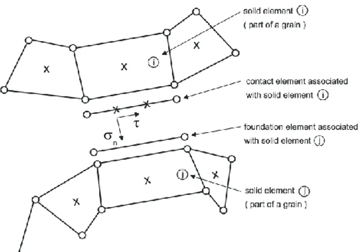
Figure 1. Interface element: contact element, associated foundation, linked solid
elements. Dots symbolize nodes and crosses represent integration points.
The interface element is composed of a modified contact element and a foundation element (see figure 1). At each iteration, the program determines the
foundation element associated to each integration point of each contact element by searching the intersection between the normal of the contact element at this integration point and the foundation elements surrounding the area. The state variables for each integration point of each interface element are computed at each iteration using information from the two solids elements in contact (elements i and j in figure 1), i.e. the solid elements attached to the contact element and foundation element determined for this particular integration point at this iteration. The state variables in the interface element are the corresponding mean values at the integration points of elements i and j. As the two surfaces of the interface can slide against each other, the foudation element facing a contact element may change during the simulation. Likewise, two integration points of a contact element may be linked to two differents foundation elements, i.e. to two different solid elements.
The original contact element was described by Habraken et al. (1998b) and is usually combined with a Coulomb’s friction law. This element has been modified in order to introduce a new interface law and a cohesion criterion. The stress components of the contact element are represented in figure 1, their evolution is described by the following viscous-elastic-type relationships:
and
s s n n c
k u u k
[2]In this penalty method the penalty coefficients ks and kn are large to keep the deviations
u u and s
c
small. u and are respectively the relative sliding velocity of adjacent grains due to shear stress and the average separation rate, normal to the interface, due to damage growth. These variables are directly computed from nodal displacements. us and are the similar variables to c u and but related to the damage law. Their evolutions are described in the section 2.2
(equations [3] and [19]). Equation [2] enforces u and to be equal to us and . c
2.2. Interface law: evolution of the damage
The major damage mechanisms at the mesoscale are viscous grain boundary sliding, nucleation, growth and coalescence of cavities leading to microcracks. The linking-up process subsequently leads to the formation of a macroscopic crack. 2.2.1. Grain boundary sliding
Grain boundary sliding is governed by:
s B u w [3]
where us is the relative velocity between two adjacent grains, w is the thickness of the grain boundary and B is the grain boundary viscosity. However wB can be expressed in term of the strain-rate parameter B defined as follows:
1 0 0 0 n n B B w d [4]
d is a length parameter related to the grain size and n is the creep exponent (Onck et al., 1999). 0, 0 are reference stress and strain-rate that depend on the steel grade. The intergranular sliding can be characterized by the ratio e B, which measures
the relative resistance between the grain and the grain boundary. In case of free sliding (B = 0), e B = 0. When there is no sliding (B), e B.
The classic creep law is defined as:
n n e e 0 e 0 B [5]Using equations [4] and [5] the ratio wB becomes:
n 1 1 n n B B w d B [6]where B is the creep coefficient.
Four parameters are then necessary to define the boundary sliding: the creep exponent n, the creep parameter B, the grain size d and the parameter characterizing the viscosity e B. The three first parameters are determined in section 3 using the
experimental results, e B is chosen equal to an intermediate value of 10 (Onck
et al., 1999).
2.2.2. Voids evolution
In the context of damage at high temperature, the mechanism of voids nucleation, growth and coalescence is established.
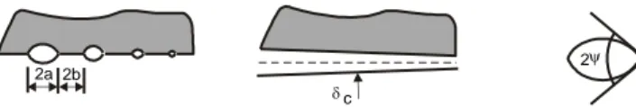
The model uses an idealized formulation of the grain boundary geometry where the cavities are supposed to be uniformly distributed on each grain boundary segment (i.e. at each integration point) with an average spacing of 2b and a diameter of 2a. Figure 2 illustrates this idealized representation: on the left each individual void is represented and on the right the voids are replaced by a continuous variable
c
elements to account for the interface thickness updating due to the presence of voids at the grain boundaries (see equation [2]). Detailed equations for the variables used for the computation of are presented in the next sections. A fracture criterion is c also proposed.
Figure 2. Discrete and continuous representations of the grain boundary (Onck et
al., 1999) and definition of
angle.2.2.2.1. Voids nucleation – computation of the cavity spacing growth rate b
In most engineering alloys, cavities have been observed to continuously nucleate. The following experimental relation has been suggested:
2 2 0 with 0 n n e n e n N F [7]
N is the average number of cavities per unit length of grain boundary. e is the equivalent creep strain rate from equation [1]. n is the normal stress, introduced to allow a faster nucleation on those grain boundaries which are perpendicular to the loading direction. is a material constant (van der Giessen et al., 1994) which is related to 0 and to Fn. 0 is a normalization constant representative of the average stress level in the material surrounding the crack. Fn is the microstructural parameter which influences the nucleation rate at the grain boundary. Zones where nucleation is more important can be introduced through this parameter. It can represent, among others, the precipitation state or the influence of the thin ferrite film that can form close to the grain boundary leading to strain concentration (Mintz et al., 1991). According to equation [7], the nucleation will begin with the plastification. However, experiment shows that nucleation appears later, that is why a threshold is used to indicate the beginning of the nucleation. For this purpose, the parameter S which combines the stress and the cumulated strain is defined:
20
n e
S [8]
The parameter S characterizes the state of the material before nucleation. It will grow with the strain until the threshold value Sthr is reached. Sthr is assumed to be related to the minimum cavity density NI from which nucleation can be observed and to the factor Fn that indicates the importance of the nucleation activity of the material:
2 2a 2b
thr I n
S N F [9]
Once nucleation begins the parameter S is not used any more in the model.
Finally, experience shows that the cavity density tends to saturate for large creep strains, then the nucleation of new cavities stops when N reaches the value Nmax. If 2b is the cavity spacing (see figure 2), N is related to it by:
2 1
N b [10]
The evolution of the cavity spacing is found by derivation of equation [10]:
1 2 N b b N [11]
By substituting equations [7] and [10] in equation [11], we have: 3 2
2 n e
b b [12] The nucleation rate N is related to the internal state of the material N as well as to the stress n and strain rate e states on the grain boundary. With a one-dimensional element, this nucleation rate N can be interpreted as a measure of the rate of evolution of the cavity spacing b. In practice, the finite element model uses equations [7] and [11] to compute the decrease rate of b due to continuous nucleation of cavities.
2.2.2.2. Voids growth – computation of the cavity size growth rate a
A detailed formulation of the cavity growth under diffusion and creep deformations was proposed by Tvergaard (1984). Assuming that a cavity is defined by two parameters : the cavity tip angle and 2a its size, the cavity growth rate is:
2 2 1 2 / 4 / 4 aV
a h VV
a h [13] where
1 1 cos 0.5 cos h sin (shape function of the cavity) and V is the
total cavity volume growth rate, which is divided into diffusion growth V (equation 1
[14]) and creep deformation V (equation [15]): 2
1 4 ln 1 3 1 2 n V D f f f [14]for for for n m m e e n m 2 e n m m e e 3 A C 1 2n 3 V A C 1 2n 3 A C 1 2n [15]
where C
n1
n0.4319
n2 and A2eCa h3
. D is a constant related to the material diffusion, n the creep exponent, n, eand m are respectively the normal, equivalent, and mean stresses applied on the grain boundary. The variable f, used in equation [14] is defined as follows:
2 2
f max a b , a a 1.5L [16] where
C
1 3 e e L D
.The coupling between diffusive and creep contribution to void growth is introduced trough the length scale L. For small values of a/L, cavity growth is dominated by diffusion while for larger values, creep growth becomes more and more important.
The diffusion parameter can be expressed as a function of the temperature by:
b0 b b D Q D exp kT RT [17]
with Db0b the grain boundary diffusion coefficient,
Ω
the atomic volume, Qb the activation energy, T the temperature in Kelvin, k = 1.3807 10-23 J K-1, the Boltzmann’s constant and R = 8.3145 J mol-1K-1, the universal gas constant. The particular values for austenitic steel are the following: Db0b= 7.5 10-14 m5 s-1, =
1.21 10-29 m3 and Qb = 159 kJ mol-1 (Needleman et al., 1980).
Finally the discrete cavity distribution is replaced by a continuous distribution on each facet of the grain boundary so that the average separation between two grains
c
, which is equivalent to a grain boundary thickness, evolves in a continuous way on the facet (see figure 2). c is determined using the volume of grain boundary cavities V and their average spacing b:
2 c V b
[18]Then, the separation rate used in equation [2] is given by: c 2 2 2 c V V b b b b [19]
To resolve the equations of this section, the following additional independent parameters have to be defined: the initial voids size a0 and spacing b0, the nucleation parameter Fn, the normalization constant 0, the cavity tip angle , the initial cavity density for nucleation NI and the maximum cavity density Nmax where nucleation stops. They are determined in section 3.3 using the damage experiments except for
, which is assumed to remain constant during voids growth and taken equal to 75° (Onck et al., 1999).
2.2.2.3. Voids coalescence and fracture criterion
Coalescence takes place when cavities are sufficiently close to each other to collapse. The parameter used to define the coalescence activation is the ratio a/b. It is called a damage variable in the current model. When this ratio reaches a critical threshold value dlim, coalescence is triggered and a crack appears. At this moment the contact is lost between the foundation and the contact element of the interface element where the criterion has been reached and a crack physically appears in the finite element model.
Preliminary simulations have been performed on simple representative cells to study and validate the model. The penalty coefficients ks and kn (equation [2]) have been defined so that the softer zone introduced in the finite element mesh due to the presence of interface elements does not influence the results before damage occurs. It has been shown that this condition is respected for ks = kn = 100000 Mpa/mm (Castagne et al., 2003). It has also been demonstrated through simulations with a mesh representing real grains that it is possible to follow the initiation and propagation of cracks with this approach (Castagne et al., 2004).
2.3. Meso-macro link
As the damage evolution is analysed at the grain scale, specific zones of study called the representative mesoscopic cells have to be defined for the finite element simulations. The macroscopic continuous casting model available at the University of Liège provides various results such as temperature field, thickness of the solidified shell, stress, strain and strain rate fields in the strand which will be used to define the thermomechanical history applied on the mesoscopic cell (Pascon et al., 2003). The macroscopic model also computes several crack risk indicators that are in agreement with observations made on industrial sites showing that transverse cracks always appear near the edge of the slab. This indicates that the mesoscopic cell has to be chosen in this zone.
To allow the transfer of data from the macroscopic model to the mesoscopic model, the mesoscopic cell has to be surrounded by a transition zone as shown in section 4.2. The history of forces and displacements are established by running a macroscopic simulation. These forces and displacements are imposed on each node of the boundary of the transition zone.
At each time step, the temperature of each node of the mesoscopic cell is fixed according to the results of the macroscopic simulation and no thermal exchange is computed at this scale as the thermal problem has already been solved by the macroscopic model.
3. Experimental analyses
The material was provided in the form of specimens cut from a rejected slab. A metallographic analysis has been preformed to establish the crystalline structure of the material. Mechanical tests have been performed to determine the material properties of the steel and damage tests have also been performed to identify the parameters that have to be introduced in the damage model.
3.1. Metallographic analysis
Metallographic analysis combining optical microscopy and picric acid etching on steel samples have been performed at room temperature to determine the original austenitic grain size and morphology.
Figure 3. Austenitic microstructure of the studied steel at mid-height of the slab
close to the lateral face on a facet parallel to this lateral face.
Figure 3 shows an example of the austenitic microstructure. The grain size was measured using the planimetric method described in the ASTM E112-96 (2004) standard. This method consists in counting the number of grains contained in a 5000 mm2 circle on an enlarged picture. Knowing the scale of the picture it is then
possible to transform this number of grains into an equivalent grain diameter. It was found that on a facet parallel to the lateral face of the slab, close to this lateral face, the grain size evolves from 1 mm at the corner of the slab to 1.5 mm in the middle, which is a huge grain size compared to the values usually found in the literature. As the cracks usually appear close to the corner of the slab, an average austenitic grain size d of 1 mm has been used in equation [4].
The austenitic microstructure (Figure 3) has also been used to define an accurate finite element mesh of the grains microstructure in the mesoscopic cell.
3.2. Mechanical analysis
Compression tests on cylindrical samples have been performed and the corresponding stress-strain curves recorded. Various strain rates (0.01, 0.001 and 0.0001 s-1) and temperatures (700, 800, 900, 1000 and 1100°C) have been used in the experimental program in order to identify the parameters p1 to p4 in equation [1]. A thermal treatment that was aimed at reproducing the thermal cycle of continuous casting had been applied on each test sample before compression.
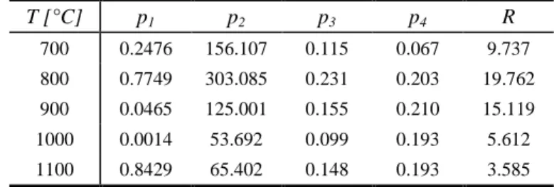
Table 1. Parameters of the Norton-Hoff law for an equivalent stress e in Mpa.
T [°C] p1 p2 p3 p4 R 700 0.2476 156.107 0.115 0.067 9.737 800 0.7749 303.085 0.231 0.203 19.762 900 0.0465 125.001 0.155 0.210 15.119 1000 0.0014 53.692 0.099 0.193 5.612 1100 0.8429 65.402 0.148 0.193 3.585
This identification has been done using a least squares method for each temperature to determine the parameters p1 to p4 of the Norton-Hoff law [1]. R2 is the variable that is minimized in the problem. It is a measure of the difference between the experimental data and the simulated curves. The results of the identification can be found in table 1. R is also given in table 1, it is a unique value for each temperature which gives an idea of the quality of the identification. R becomes zero when the difference between the data points and the fitted curve is zero.
The softening parameter p1 does not influence the results of the macroscopic continuous casting model as it has principally an effect in the large strains that will not appear in this process. Nevertheless, it is important to have an accurate model at larger strains for the acoustic tests simulations used to identify the damage
parameters and in case of localised higher strains due to the grain configuration in the mesoscopic cell. The evolution of p2, which is correlated to the maximum value of the stress, is consistent with the presence of the ductility gap leading to higher stresses at 800°C. The viscosity parameter p3 and the hardening parameter p4 lie almost in the interval 0.1 – 0.2, which fits with usual values found for steel. p3 does not increase monotonously as could have been expected for the majority of steel grades. This type of behaviour has also been found in the literature for several low carbon steel grades(Altan et al., 1983), which is the type of steel used in this study.
Figure 4 shows the results of the calibration at T=1100°C for 3 strain rates. The oscillating lines correspond to the experimental results and the smooth lines to the Norton-Hoff curves (equation [1]) using the parameters of table 1.
Figure 4. Experiments and Norton-Hoff curves at T=1100ºC.
The results of the mechanical experiments have also been used to determine the creep parameters of the interface model. Even if the curve shape could suggest that some recrystallization occurs, this phenomena is neglected in the model The creep parameters B and n can be determined using the Norton-Hoff law. The Norton-Hoff law [1] is different from the classic creep law [5] but the two formulations can be linked together if some assumptions are made. The Norton-Hoff links the equivalent stress to the equivalent strain and strain rate whereas the classic creep law only links the equivalent stress with the equivalent strain rate. For a given value of the strain
e
, equation [1] can be rewritten:
3 1 p e e [20] 0 5 10 15 20 25 30 35 40 0 0.1 0.2 0.3 0.4 0.5 0.6 0.7 eq eq [Mpa] eq= 0.01 /s eq= 0.001 /s eq= 0.0001 /sand n can be identified by comparison of equations [5] and [20]: 3 1 n p [21]
Although B is a function of the equivalent strain e, a unique value of B has been determined corresponding to a representative strain for this problem. e= 0.07 has been chosen as it corresponds to the value for which the stress reaches a plateau and B becomes quasi-independent of e. It is also of the order of magnitude of the strains found in continuous casting. Knowing p1 to p4 and e, B can be found by
identification of equations [1] and [5]. The normalization constant 0 is computed using the same method. 0 has to be representative of the stress level in the material and is therefore computed using the Norton-Hoff law with a strain e= 0.07 and an intermediate strain rate e= 10-3 s-1. The values of n, B and 0 are given in table 2. As in table 1, the units in table 2 are consistent with an equivalent stress in Mpa.
Table 2. Parameters n, B and Σ0.
T [°C] n B Σ0 [Mpa] 700 8.696 2.263E-21 106.955 800 4.329 1.270E-11 66.683 900 6.452 1.821E-14 46.202 1000 10.081 1.461E-18 29.625 1100 6.757 3.642E-13 24.941 3.3. Damage analysis
The damage analysis consists in acoustic tests realised in order to determine the apparition of the first crack during the compression of steel samples. At the origin, these tests were developed at IBF (RWTH-Aachen) to predict the formality of steel at low temperature and were then adapted to the conditions prevalent during hot forming (Kopp et al., 1999).
If the internal stresses in a crystal are exceeding locally a critical threshold during forming, a sudden change appears (the initiation of a micro-crack), which allows the material to go back to an equilibrium state with a lower potential energy. The potential energy emitted is dissipated in the form of elastic waves that can be detected in the surrounding area as sound pulses. Piezoelectric sensors are used to record the sound signals. These signals, that have a very low intensity, are
pre-amplified, filtered to separate the sound associated with the damage process from the interferences and amplified again before being introduced in the data acquisition system.
In order to reproduce the continuous casting conditions and the microstructure of the steel during this process, the samples were first heated up to 1375°C in an external radiation furnace and maintained at this temperature for ten minutes before cooling down to test temperature. To protect the sample material against surface oxidation, the furnace was rinsed with argon inert gas. Afterwards the samples were manually placed in the compression machine. The surrounding furnace was heated up to test temperature within the argon atmosphere. Finally the samples were compressed up to crack initiation with a constant strain rate while upcoming acoustic emission events causes by material failure were recorded.
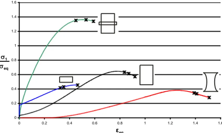
Several sets of acoustic tests have been done with different sample geometry (two cylindrical: flat and slim and two non-cylindrical: flange and concave shapes) to generate different stress-strain histories at the critical point of the samples (see figure 5). The critical point is the point where the crack is supposed to appear due to the mechanical loading, i.e. where the maximum principal stress will reach its maximum value (on the outer edge at mid-height for the flat, slim and concave samples and at the intersection of the outer edge of the cylindrical part with the ring for the flange sample). The location of the critical point has been determined experimentally for various samples at the time of the development of the technique at IBF.
Three temperatures (800°C, 900°C, 1000°C) and two strain rates (1·10-3 s-1, 5·10-4 s-1) have been tested with at least three samples for each combination and for each geometry to ensure statistically relevant results.
4. Finite element analysis
The parameters are identified using a reverse method that requires two major steps. First the loadings to be applied to the mesoscopic cell have to be determined by macroscopic simulations of the acoustic tests and then these data have to be transferred to the mesoscopic cell to solve the reverse problem.
4.1. Macroscopic modelling of the acoustic tests
The finite element simulations of the acoustic tests give the formability curves and also the stress, strain and temperature fields in the whole sample and in particular in the region where the crack is expected to appear. The material law used for these simulations is the elastic-viscous-plastic law that is also used to model the grains behaviour of the mesoscopic model (see equation [1]). The temperature is fixed at the corresponding test temperature for each simulation. The compression
0 0.2 0.4 0.6 0.8 1 1.2 1.4 1.6 0 0.2 0.4 0.6 0.8 1 1.2 1.4 1.6 1 eq eq ε
load is modelled using a tool whose displacement produces a vertical logarithmic strain in the sample corresponding to the required constant strain rate. A contact law with friction is used between the sample and the tool.
A sensitivity analysis has shown that the results where strongly dependent on the friction coefficient between the tool and the sample. Therefore, further experiments performed at IBF using the same procedure as for the acoustic tests have been necessary to determine the actual friction coefficient. The chosen tests were ring tests at 800 °C and with a constant displacement rate of the tool of 8·10-3 mm s-1. The friction coefficient found is 0.2.
Figure 5 shows the evolution of the specific maximal principal stress versus the equivalent strain at the critical point for a temperature of 900°C and a strain rate
= 5·10-4 s-1, these results have been obtained by finite element simulations of the compression tests for each sample geometry. The crosses on the curves in figure 5 indicate the moment of the first crack initiation for each test (three samples tested for each combination of temperature and strain rate).Figure 5. Macroscopic simulations (T = 900°C,
= 5·10-4 s-1).Different element sizes have been tested in the critical zone and the stress and strain fields compared in order to analyse the mesh dependence of the results. For the slim, flat and concave samples, a threshold (0.2 mm x 0.2 mm) has been determined for the minimum size of the elements under which it is not necessary to go as the results of the simulations in term of stresses and strains distributions remain similar. For the flange sample, the stress concentration is so high in the critical zone that it was not possible to find a mesh with a reasonable number of elements for which the results converged with a sufficiently high accuracy. Therefore, it has been decided to keep only the three first samples, which give reliable results, for the identification stage.
4.2. Mesoscopic simulation of the acoustic tests
4.2.1. Transfer of data
A surrounding transition zone is used to transfer the data from the macroscopic model to the mesoscopic model (figure 6). From a mechanical point of view, the mesoscopic cell is a slice in generalised plane strain state. This formulation allows applying non null stresses and strains simultaneously in the out-of-plane direction (Pascon et al., 2003). The history of forces and displacements are determined by running macroscopic simulations and are used as boundary conditions imposed on each node of the periphery of the transition zone. As an elastic-viscous-plastic constitutive law is used in the grains and the damage variables at the interfaces grow during the loading, it is important to follow the whole forming process.
Figure 6. Left: mesoscopic cell surrounded by a transition zone (50 mm x 50 mm).
Right: zoom on the grains (5 mm x 5 mm).
For the acoustic tests simulations, the temperature is fixed and is constant in the specimen. Nevertheless, the method could be used for simulations with variable temperatures, the temperature of each node of the mesoscopic cell should be fixed at each time step according to the results of the parent macroscopic simulation. No thermal exchange is computed at the mesoscopic scale as the thermal problem has already been solved by the macroscopic model.
During the data transfer, the objective is to reproduce in the mesoscopic cell the stress and strain tensors histories recorded at the critical point of the parent macroscopic simulation. These mechanical fields are assumed to be uniform on the cell with small variations in the grains zone due the grains pattern and to the damage initiating at the grain boundaries. The loading can be applied using forces or displacements or a combination of the two. The stress-strain fields are three-dimensional in the macroscopic simulations, with compression in the axial direction and tension in both radial and circumferential directions. In the critical element, the radial stress vanishes as the edge of the sample is reached but the strain field remains three-dimensional. The compression stress is reproduced on the mesoscopic cell in the direction normal to the plane (z direction) using the properties of the
x y
generalised plane strain state. The tensile stress, which is responsible for the apparition of the crack, is applied in the y direction of the mesoscopic cell. The stress in the x direction and the shear stresses have to be equal to zero.
For the first trial, displacements were imposed in the three directions as the simulations usually have a better convergence when the loadings are imposed through displacements only. Although the correct equivalent stress was computed in the mesoscopic cell, it appeared that the stress components distribution was not correct. This is due to the formulation of the elastic-viscous-plastic law, which is given in terms of equivalent stress and strain. Indeed, different stresses distributions can correspond to the same equivalent stress.
It has been found that the correct stress and strain tensors can be reproduced if a displacement is imposed in the x direction and forces in the y and z directions. This has been verified by plotting these fields for the critical point of the macroscopic simulations and for the elements of the transition zone of the mesoscopic cell. For this analysis, damage parameters from the literature have been used. Looking globally at the mesoscopic cell, it has been shown that the results of the data transfer were not dependent on the damage parameters as the influence of damage on the macroscopic stresses is negligible.
4.2.2. Sensitivity analysis
Figure 7 represents a typical damage evolution. Three phases can be defined. First the damage increases very slowly due the diffusion of voids and to the growth of the voids that are already present (A-B). Then the nucleation threshold is reached, new voids are created and the damage increases more rapidly (B-C). Finally, the saturation state is reached, no more cavities can be created and the growth of the damage slows down until final rupture (C-D).
Figure 7. Typical damage evolution. 0 0.1 0.2 0.3 0.4 0.5 0.6 0.7 0.8 0 200 400 600 800 1000 1200 1400 Time (s) D a m a g e A B C D
The damage parameter is the ratio between the voids diameter 2a and the average spacing between voids 2b. The initial damage value depends on the initial values a0 and b0. The initial density of cavities for nucleation by unit length NI and the nucleation activity parameter Fn determine the position of point B. The slope of the curve between B and C partially depends on the value of Fn. The maximum density of cavities Nmax influences strongly the position of point C. These five parameters (a0, b0, NI, Fn and Nmax) and the damage threshold for crack appearance
dlim have not been fixed yet and can be used for the calibration of the model. The diffusion and creep parameters that also influence the damage curve have already been fixed (see section 2.2).
4.2.3. Results of the identification
First, the mesoscopic cell has been loaded using the results of the acoustic simulations at T = 900°C,
= 5·10-4 s-1 for the three samples shapes (slim, flat and concave) and a range of damage parameters have been tested to reproduce the experimental results, i.e. so that the first crack appear at the expected time for each geometry. Then, the set of parameters that best fitted the experiments has been tested for the other combinations of temperature and strain rate and the parameters have been further optimized.The final parameters determined by the acoustic analysis are the following: a0 = 2.75·10-3 mm, b0 = 2.75·10-2 mm, NI = 380 mm-1, Fn = 1.5·105 mm-1, Nmax= 40 NI and
dlim= 0.7. Even if the numerical model allows a temperature dependence of these parameters, a unique set of parameters could be established. The temperature dependence is already modelled through the diffusion and creep parameters.
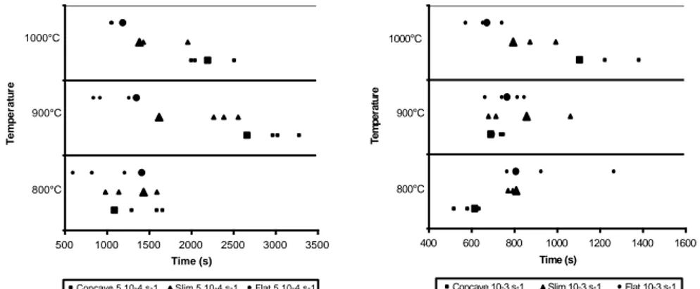
Figure 8. Time of crack appearance: comparison model and experiments for
= 5·10-4 s-1(left) and
= 1·10-3 s-1(right). The small symbols represent the experiments while the corresponding large symbols represent the model.500 1000 1500 2000 2500 3000 3500
Concave 5 10-4 s-1 Slim 5 10-4 s-1 Flat 5 10-4 s-1 1000°C 900°C 800°C Time (s) T e m p e ra tu re 400 600 800 1000 1200 1400 1600
Concave 10-3 s-1 Slim 10-3 s-1 Flat 10-3 s-1 1000°C 900°C 800°C Time (s) T e m p e ra tu re
Figure 8 compares the results of the experiments (small symbols) with the results of the identified model (large symbols). With this set of parameters, the model predictions match the experiments quite well. The largest differences are for the concave and slim samples at T = 900°C and
= 5·10-4 s-1 for which the model predicts the crack too early. For the other combinations of parameters, the simulations results correspond to the data points except for the flat sample at
= 5·10-4 s-1 for which the model predicts the crack a little bit later than what has been experimentally observed. In global, the set of parameters is considered to be representative of the experiments.5. Conclusions
A model for crack initiation and propagation in steel at high temperature has been developed. Experimental results and a reverse method have been used to identify the mechanical and damage parameters at elevated temperature. The identified finite element model has shown that it gives good results. This validated model will now be used to investigate the apparition of cracks in continuous casting and in particular the link between the intergranular crack appearance at the mesoscopic level and different macroscopic factors such as the shape of oscillations marks and the thermo-mechanical history during the process.
Acknowledgements
As Research Associate, A.M. Habraken would like to thank the Belgian National Fund for Scientific Research for its support. The industrial partner ARCELOR is also acknowledged as well as IBF (RWTH-Aachen) and the Department of Metallurgy and Materials Science of the University of Liège who contributed to the experimental part of this study.
6. References
Altan T., Oh S. and Gegel H., Metal Forming Fundamentals and Applications, published by ASM International, 1983, p. 60-61.
Anonymous, “Standard Method for Determining Average Grain Size”, ASTM E112-96, published by ASTM International, 2004.
Brimacombe J.K and Sorimachi K., “Crack Formation in the Continuous Casting of Steels”,
Metallurgical Transactions B, vol. 8 no. 3, 1977, p. 489-505.
Castagne S., Pascon F., Blès G. and Habraken A.M, “Developments in Finite Element Simulations of Continuous Casting”, Journal de Physique IV, vol. 120, 2004, p. 447-455.
Castagne S., Remy M. and Habraken A.M, “Development of a Mesoscopic Cell Modelling the Damage Process in Steel at Elevated Temperature”, Key Engineering Materials, vol. 233, 2003, p. 145-150.
Habraken A.M., Charles J.F., Wegria J. and Cescotto, S., “Dynamic Recrystallisation during Zinc Rolling”, Int. J. Forming Processes, vol. 1 no. 1, 1998a, p. 53-73.
Habraken A.M. and Cescotto S., “Contact between Deformable Solids: the Fully Coupled Approach”, Mathl. Comput. Modelling, vol. 28 no. 4-8, 1998b, p. 153-169.
Kopp R. and Bernrath G., “The Determination of Formability for Cold and Hot Forming Conditions”, Steel Research, vol. 70 no. 4-5, 1999, p. 147-153.
Mintz B., Yue S. and Jonas J.J., “Hot Ductility of Steels and its Relationship to the Problem of Transverse Cracking during Continuous Casting”, Int. Mater. Rev., vol. 36 no. 5, 1991, p. 187-217.
Needleman A. and Rice J.R., “Plastic Creep Flow Effects in the Diffusive Cavitation of Grain Boundaries”, Acta Metallurgica, vol. 28 no. 10, 1980, p. 1315-1332.
Onck P. and van der Giessen E., “Growth of an Initially Sharp Crack by Grain Boundary Cavitation”, J. Mech. Phys. Solids, vol. 47 no. 1, 1999, p. 99-139.
Pascon F. and Habraken A.M., “2D½ Thermo-Mechanical Model of Continuous Steel Casting Using F.E.M.”, in Proc. 6th
Esaform Conference on Metal Forming, Salerno,
Italy, edited by V. Brucato at Nuova Ipsa Editore, 2003, p. 759-762.
Suzuki H., Nishimura S., Imamura J. and Nakamura Y., “Embrittlement of Steels occurring in the Temperature Range from 1000 degrees-C to 600 degrees-C”, Transaction ISIJ, vol. 24 no. 3, 1984, p. 169-177.
Tvergaard V., “On the Creep Constrained Diffusive Cavitation of Grain Boundary Facets”, J.
Mech. Phys. Solids, vol. 32 no. 5, 1984, p. 373-393.
van der Giessen E. and Tvergaard V., “Development of Final Creep Failure in Polycrystalline Aggregates”, Acta Metall. Mater., vol. 42 no. 3, 1994, p. 959-973.
Zhu Y. and Cescotto S., “Unified and Mixed Formulation of the 4-Node Quadrilateral Elements by Assumed Strain Method: Application to Thermomechanical Problems”, Int.

![Figure 4 shows the results of the calibration at T=1100°C for 3 strain rates. The oscillating lines correspond to the experimental results and the smooth lines to the Norton-Hoff curves (equation [1]) using the parameters of table 1](https://thumb-eu.123doks.com/thumbv2/123doknet/6555941.176943/12.892.238.658.491.736/figure-results-calibration-oscillating-correspond-experimental-equation-parameters.webp)