Simulation of the VVER-1000 pump start-up experiment in the OECD/DOE/CEA V1000CT benchmark by the FLICA4/CRONOS2 coupled code system

HAL Id: cea-02356018

https://hal-cea.archives-ouvertes.fr/cea-02356018

Submitted on 9 Dec 2019

HAL is a multi-disciplinary open access archive for the deposit and dissemination of sci-entific research documents, whether they are pub-lished or not. The documents may come from teaching and research institutions in France or abroad, or from public or private research centers.

L’archive ouverte pluridisciplinaire HAL, est destinée au dépôt et à la diffusion de documents scientifiques de niveau recherche, publiés ou non, émanant des établissements d’enseignement et de recherche français ou étrangers, des laboratoires publics ou privés.

FLICA4/CRONOS2 coupled code system

Sylvie Aniel-Buchheit

To cite this version:

Sylvie Aniel-Buchheit. Simulation of the VVER-1000 pump start-up experiment in the

OECD/DOE/CEA V1000CT benchmark by the FLICA4/CRONOS2 coupled code system. Progress in Nuclear Energy, Elsevier, 2006, 48 (8), pp.773-789. �10.1016/j.pnucene.2006.06.006�. �cea-02356018�

SIMULATION OF THE VVER-1000 PUMP STARTUP

EXPERIMENT IN THE OECD/DOE/CEA V1000CT BENCHMARK

BY THE FLICA4/CRONOS2 COUPLED CODE SYSTEM

Sylvie Aniel

DM2S/SFME/Laboratoire d'Etudes Thermiques des Reacteurs CEA Saclay - 91 191 Gif sur Yvette Cedex – France

Phone : (33)169086488 Fax : (33)169088568

saniel@cea.fr ABSTRACT

In the framework of joint effort between the Nuclear Energy Agency (NEA) of OECD, the United States Department of Energy (US DOE), and the Commissariat à l’Energie Atomique (CEA), France a coupled 3-D thermal hydraulics/neutron kinetics benchmark was defined. The overall objective of OECD/NEA V1000CT benchmark[7] is to assess computer codes used in the analysis of VVER-1000 reactivity transients where mixing phenomena (mass flow and temperature) in the reactor pressure vessel are complex. Original data from the Kozloduy-6 Nuclear Power Plant are available for the validation of computer codes: one experiment of pump start-up (V1000CT-1) and one experiment of steam generator isolation (V1000CT-2). The CEA presented results for the V1000CT-1 Exercise 2 using a coupling of FLICA4[3] and CRONOS2[2] via the coupling tool ISAS[4. The FLICA4/CRONOS2 VVER-1000 model is based on the data available in the benchmark specifications. This paper summarizes the FLICA4/CRONOS2 model build-up with the associate sensitivity studies and presents the CEA results for V1000CT-1 Exercise 2 as well as a comparison with experimental results at Hot Power Steady State (HP SS).

KEYWORDS

1. INTRODUCTION

The CEA participated in V1000CT-1 by submitting results for Exercise 2 and by collaborating in the participants’ results analysis[1]. This paper focuses on the CEA results for V1000CT-1 Exercise 2[6. After a brief presentation of the FLICA4 and CRONOS2 codes and the ISAS coupling tool, the first part describes, in manner as exhaustive as possible, the coupled reference model used to obtain the submitted results for code to code and code to experiment comparisons. The second part presents the sensitivity studies used to assess the modeling choices. The FLICA4/CRONOS2 V1000CT-1 Exercise 2 results are shown in a third part before a comparison with experimental results at Hot Power (steady state).

2. FLICA4/CRONOS2 REFERENCE MODEL

2.1 Codes presentation

FLICA4[3], CRONOS2[2] and ISAS[4] are part of the SAPHYR[5] system. SAPHYR codes are based on a modular structure that allows a great flexibility of use. A special user-oriented language, GIBIANE, and a shared numerical toolbox have been developed to chain the various computation modules.

CRONOS2 has been designed to provide all the computational means needed for nuclear reactor

core calculations, including design, fuel management, follow-up and accidents. CRONOS2 allows steady state, kinetic, transient, perturbation and burn-up calculations. The power calculation takes the thermal-hydraulic feedback effect into account, either by a 1-D simplified model, or by the coupling with FLICA4. All of this can be done without any limitation of any parameter (angular discretisation, energy groups, spatial meshes). The code solves either the diffusion equation or the even parity transport equation with anisotropic scattering and sources. Different geometries are available such as 1-,2- or 3-D Cartesian, 2- or 3-D hexagonal and cylindrical geometries. Four different solvers are available : PRIAM, MINOS ,CDIF and VNM. The PRIAM solver is used for hexagonal geometries. It uses the second order form of the transport equation and is based on SN angular discretisation and a finite element

approximation on the even flux (primal approximation).

FLICA4 is a 3-D two-phase compressible flow code especially devoted to reactor core analysis.

mixture and mass conservation of the vapor. The velocity disequilibria are taken into account by a drift flux correlation. A 1-D thermal module is used to solve the conduction in solids (fuel). Thanks to the modular design of the SAPHYR codes, numerous closure laws are available for wall friction, drift flux, heat transfer and critical heat flux (CHF). A specific set has been qualified in FLICA3 for PWR applications. An extensive qualification program for FLICA4 is under way, based on recent experimental data, in order to cover a wider range of flow conditions. FLICA4 includes an object-oriented pre-processor to define the geometry and the boundary conditions. Radial unstructured meshes are available, without any limitation of the number of cells. Zooming on a specific radial zone can be performed by a second calculation using a finer mesh (for instance a sub-channel calculation on the hot assembly). The fully implicit numerical scheme is based on the finite volumes and a Roe solver. This kind of method is particularly accurate, with a low numerical diffusion.

ISAS is a general coupling tool based on the Parallel Virtual Machine (PVM) data exchange

protocol, and provides a supervision language (GIBIANE or OCAML). Each coupled code remains independent, and is run as an individual process within a master-slave relationship. As long as an ISAS interface exists in a code, this code can be coupled to any other code through ISAS without any more specific developments. This applies very conveniently to modular codes such as CRONOS2 and FLICA4.

2.2 Coupled reference model

The physical modeling was done using as much as possible the specifications data[6]. The numerical models were chosen to reach the highest level of precision compatible with a reasonable computation time. The numerical convergence was estimated (see §4).

2.2.1 Neutronic modeling:

The radial core description is nearly identical to the specification data : the core heated part is described by 163 fuel assemblies and 54 assemblies are placed around to represent the radial reflector (6 reflector assemblies are added because the hexagonal geometries are described by rings in CRONOS2). Their radial dimensions are as specified in the benchmark. The axial physical meshing is as specified (10 layers for the heated core and 2 layers for the lower and upper axial reflectors). A specific tools has been developed to take the benchmark cross sections as neutronic data (for both fuel and reflector assemblies).

The CRONOS2 interpolation procedure was successfully checked by comparison with the results of the Pennstate University (PSU) interpolation procedure ([1]). The control rod insertion in an axial mesh is taken into account by doing an interpolation between the rodded and unrodded cross-sections using the ratio between the rodded length and the axial mesh length. As in the specifications, zero flux boundary conditions are taken on outer reflector surface for both radial and axial reflectors.

The PRIAM solver is used. Radially, the hexagonal calculations are done using the standard parabolic Lagrangian finite elements with 19, 61 or 127 nodes per hexagon (depending if hexagons are divided in 1, 2 or 3 calculation meshes) (see [1] for more details). The reference model uses 61 nodes per hexagon (the physical mesh, that is to say the hexagon, is divided in 2 calculation meshes). Axially, the reference model divides the axial meshes in two and uses parabolic polynomials.

2.2.2 Thermal-hydraulic modeling:

A 3-D physical description of the 163 coolant channels (corresponding to the 163 Fuel Assemblies (FAs)) is done in FLICA4. The total height of fuel assembly (as described in the specifications), going from the bottom of the bottom nozzle to the top of the top nozzle, is modeled. The assembly axial meshing is given in table 1. The channels thermal-hydraulic characteristics (flow areas, hydraulic diameters, singular pressure losses...) are derived from the benchmark specifications. The benchmark specifications are applied for the dimensions and the thermal properties of the fuel rods materials and of the fuel gap. The Doppler temperature is calculated with the benchmark formula.

The benchmark boundary conditions are applied to the bottom of the bottom nozzle (the inlet mass flow rate and the inlet coolant temperature) and to the top of the top nozzle (outlet coolant pressure).

A precision of 10-4 kg/ m3 is required for convergence of steady state runs.

2.2.3 Coupling scheme:

The diagram of the FLICA4/CRONOS2 iteration for steady state calculations is given in figure 1. The convergence criteria are the followings:

-evolution of CRONOS2 convergence criteria: the first iteration starts with a required precision of 10

-3

on the eigenvalue and on 10-2 on the flux. The required precision is divided by 2 at each N/TH iteration to reach 10-5 for the eigenvalue and 10-4 for the flux.

- criterion on the 3D power map evolution between 2 N/TH iteration : the maximum authorized local 3-D difference in the power between 2 iterations is 0.1%. But the required precision on the flux is low enough to enable a higher stabilization of the power map. The criteria on the power map convergence is thus of no use in this case.

The diagram of the FLICA4/CRONOS2 exchanges versus time is given in figure 2. The transient time scheme is fully explicit. At each time step, FLICA4 gives the 3-D feedback effects (fuel Doppler temperature and moderator density) to CRONOS2 via ISAS, CRONOS2 sends back the 3-D power distribution and the fission power level to ISAS and ISAS sends to FLICA4 the CRONOS2 3-D power distribution and the sum of the fission power level and the decay heat (use of the benchmark decay heat versus time curve). A transient with steady state boundary conditions (SS BC) is always run before the Exercise 2 specified transient to check the stability of the steady state conditions. The transient , as specified in the benchmark, starts at 0. The time step is 0.2s from –0s to 20s and 1s from 20s to 800s.

3. FLICA4/CRONOS2 RESULTS 3.1 V1000CT1-Exercise2 results

The results of the FLICA4/CRONOS2 modeling of V1000CT1-Exercise2 are given below to enable a complete comparison with other coupled codes results.

3.1.1 Results at Hot Zero Power (HZP)

Integral parameters:

Eigenvalue (keff) 0.99963 Radial power peaking factor 1.405 Axial power peaking factor 1.523

Axial offset -16.81

Ejected rod worth, %(dk/k) 0.0893 Control rod group #10, %(dk/k) 0.69112 Tripped rods worth, %(dk/k) 7.0116

Power distributions :

The 2-D radial power distribution at steady state Hot Zero Power is given in figure 3 and the corresponding axial power profile is given in figure 4.

3.1.2 Steady state and Transient results at Hot Power

Integral parameters

Time = 0 s Time = 15 s Time = 800 s Eigenvalue (keff) 1.00170

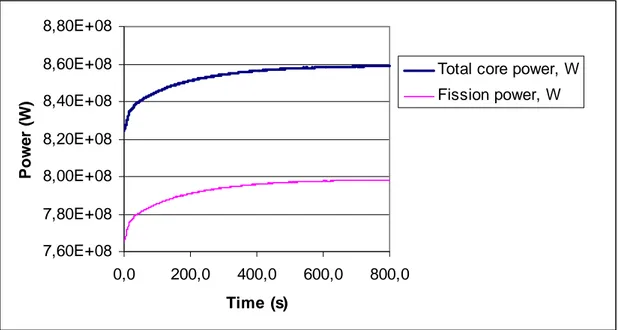
Radial power peaking factor 1.346 1.358 1.351 Axial power peaking factor 1.44 1.432 1.43 Axial offset -18.48 -17.49 -17.29 Total core power [MW] 824 834.5 858.9 Fission core power [MW] 765.4 775.6 798.2 Core average fuel temp. [K] 597.1 595.9 596.9 Core average moderator density [kg/m3] 754.8 757.8 758.1 Maximum nodal fuel temperature [K] 631.9 631 633

Power Distributions

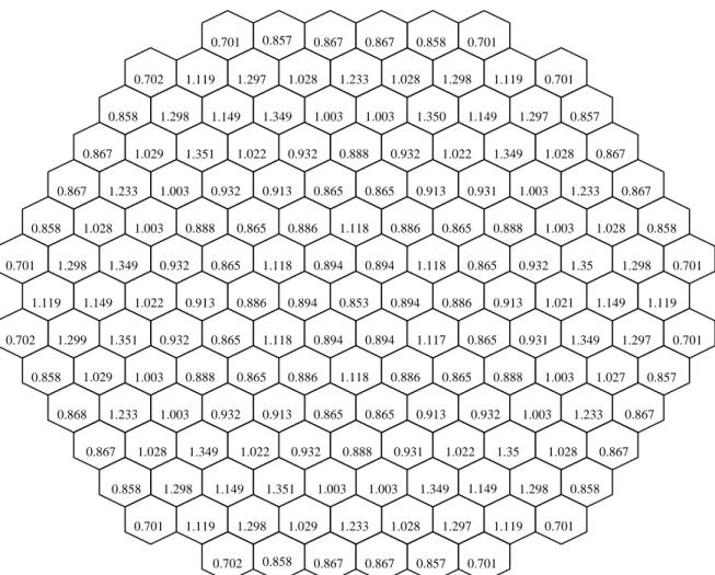
The evolution of the axial power profile during transient at Hot Power is given in figure 5. Figures 6,7 and 8 show the 2-D radial power distribution at different times of the transient.

Power level

The evolution of the core total power and of the fission power as a function of time are given in figure 9. Physical parameters

The time dependence of the average and maximum fuel temperatures and of the average coolant density is respectively given in figures 10 and 11.

3.2 Comparison with Experimental data at HP SS

The FLICA4/CRONOS2 results are compared to plant data obtained at HP SS.

As an uncertainty remained on the real position of the control rod group #10 (36% withdrawn or 36% inserted) experimental measurements are compared with two FLICA4/CRONOS2 simulations corresponding to the two possible positions of control rod group #10. Figure 12 and 13 give a comparison of the power maps. Figure 12 shows discrepancies randomly distributed over the core and a power underestimated in FAs close to the control rods group #10 positions. Figure 13 shows a clear and regular swinging from the peripheral zone to the center one. These comparisons prove that the control rods are 36% inserted in the experiment. Figure 14 shows that the discrepancies observed on core outlet temperatures (FLICA4/CRONOS2 model with control rod group #10 36% inserted) are not significant. As sensitivity studies highlight (see §4), the radial power map is not significantly affected by the feedbacks modeling, the observed swinging from the peripheral zone to the center one is certainly due to the neutronic modeling and more precisely to the reflector. The process for reflectors cross-sections build-up is described in reference [1]. As the spatial convergence of CRONOS2 modeling has already been tested (see §4) there is no reason for the CRONOS2 solution to differ from the analytical solution. The most probable source of error lies in the description of the reflector made in the HELIOS calculations. It would probably be worth to make tests on the reflector modeling and to refine its description if possible.

4. SENSITIVITY STUDIES 4.1 Convergence tests

4.1.1 Neutronic radial modeling

The reference model uses 61 nodes per hexagon (which is equivalent to 2 calculation meshes per hexagon (see [1])) with parabolic Lagrangian polynomials. A HP SS calculation has been performed with 127 nodes per hexagon (equivalent to 3 calculation meshes per hexagon) with the same polynomials. The discrepancies in term of eigenvalue and power distribution have the same order of magnitude as the required precisions. The convergence on the radial calculation meshing is thus reached with 61 nodes per hexagon when parabolic Lagrangian polynomials are used.

The reference model uses 2 calculation meshes per axial mesh and parabolic polynomials. A test using 4 calculation meshes per axial mesh with the same polynomials has been performed. The results are the following:

Comparisons on integral parameters:

The discrepancies, given in table 2, are negligible. Comparisons on power maps:

Table 3 gives the comparison of the axial power profiles. Differences are the highest in areas with the highest flux gradients (close to the axial reflectors). But they are kept reasonable knowing that theses zones are the ones having the lower power level.

The discrepancies observed on the 2-D radial power are not higher than 0.1% Impact on thermal-hydraulic parameters:

The moderator density and the fuel temperature are only slightly modified.

The computation time being about 4 times higher when changing from 2 to 4 calculation meshes per axial node and the discrepancies being kept very low, 2 calculation meshes per axial node were judged to be enough.

4.1.3 Thermal-hydraulic axial modeling.

A test has been done to check the FLICA4 axial discretization. The CRONOS2 and FLICA4 axial reference physical mesh size was divided by 2. For Cronos2 it is equivalent to have 4 axial calculation meshes per axial reference node. The steady state hot zero power results with the FLICA4 axial reference physical mesh size correspond thus to the results obtained for § 4.1.2 comparisons. It was thus possible to separate the impact of the FLICA4 axial modeling. The results are the following:

Comparisons on integral parameters:

Table 4 gives the influence of the FLICA4 meshing on the integral parameters. Comparisons on power maps:

Table 5 gives the comparison of the axial power profiles. Differences are again the highest in areas with the highest flux gradients (close to the axial reflectors). However the discrepancies can also reach 1.35% in the zone of higher power.

The discrepancies observed, on the 2-D radial power, between 1 FLICA4 axial mesh and 2 FLICA4 axial meshes per axial node, are not higher than 0.8%. The discrepancies observed, on the 2-D radial power, between 2 FLICA4 axial meshes per axial node and the reference model, are not higher than 0.9%. The impact on the radial power map is thus lower than the impact on the axial power profile. Impact on thermal-hydraulic parameters:

The discrepancies observed, on the local 3-D fuel Doppler temperatures, between 1 FLICA4 axial mesh and 2 FLICA4 axial meshes per axial node, are not higher than 0.36%. The discrepancies observed, on the local 3-D fuel Doppler temperatures, between 2 FLICA4 axial meshes per axial node and the reference model, are not higher than 0.37%.

The discrepancies observed, on the local 3-D moderator densities, between 1 FLICA4 axial mesh and 2 FLICA4 axial meshes per axial node, are not higher than 0.12%. The discrepancies observed, on the local 3-D moderator densities, between 2 FLICA4 axial meshes per axial node and the reference model, are not higher than 0.12%.

The reference FLICA4 axial meshing is less converged than the CRONOS2 one. The discrepancies are still weak and not worth the increase of computation time. The impact on the V1000CT1-Exercise2 transient results should also be low, but noticeable, if one refers to §4.2.2 steady state and transient results.

4.1.4 Convergence test on time step for transient runs

A transient has been run with a time step divided by 2: 0.1 s from –0s to 20s and 0.5s from 20s to 800s. But the observed discrepancies are not significant (< 0.1%).

4.2 Sensitivity to physical parameters

4.2.1 Sensitivity to the Doppler temperature formula: The formula given in the benchmark specifications is :

Tf = (1-a)T fuel center + aT fuel surface with a=0.7 The Rowland’s formula is:

Tf = 4/9 T fuel center + 5/9T fuel surface

Applying the Rowland’s formula instead of the one given in the benchmark specifications leads to no significant discrepancies (< 0.1%).

4.2.2 Sensitivity to the gap width between fuel and clad

The gap width has been decreased by a factor 2. The observed discrepancies are noticeable but still weak as show the tables 6,7 and 8 and the figures 15 to 18 .Table 6 shows a discrepancy of 59 pcm which is noticeable. The study of table 6 shows that this variation is due to a modification of the axial power profile, the radial power shape being only slightly affected. A decrease of the gap width leads a decrease of the fuel temperature. That is in favor of axial zones with the highest power since they have the highest fuel temperature as verified on table 8. The 2-D radial power map is only slightly modified (discrepancies<0.2%). Figure 15 shows that the discrepancies on the axial power profile reaches 2%, but in a zone of lower power. They are kept below 1% in the axial zones of high power. The axial power profile stays stable versus time but the TH boundary conditions changes are two weak to draw any kind of conclusion. Figure 16 shows however that the discrepancy on the total power reaches 2.5% at the end of the transient. The global behavior of the core is thus affected by the modification of the axial power profile (as it was already noticed with the modification of the eigenvalue). Figure 18 shows a noticeable modification of the Doppler fuel temperature with the gap width change that stay stable during the transient. This translates a change in the fuel temperature profile that stays stable since the transient is slow enough to be considered as a succession of steady-states. Figure 17 confirms that all the additional power is transmitted to the fluid.

5. CONCLUSIONS

A reference FLICA4/CRONOS2 model of the VVER-1000 has been defined. The FLICA4/CRONOS2 code convergence has been verified and the precision of the reference model determined.

The sensitivity to the Doppler temperature formula and to the fuel gap width has also been estimated. But only the gap width has a real impact on the steady state and transient results.

The results of the reference FLICA4/CRONOS2 model were compared to other codes results in the frame of the V1000CT-1 Exercise2 benchmark. They were reasonable.

The comparison with experimental results show reasonable discrepancies (kept below 10%, with a mean value around 5%). A large swinging from the peripheral zone to the center one is observed. The previous sensitivity studies (see [1]) lead to take interest in the physical description of the radial reflector made in the HELIOS calculations used in the process of reflector cross-sections build-up.

NOMENCLATURE

1-D One-Dimensional 2-D Two-Dimensional 3-D Three-Dimensional CEA Commissariat à l'Energie Atomique DOE Department of Energy

FA Fuel Assembly

FEM Finite Element Method

HP Hot Power

HP SS Hot Power Steady State

HZP Hot Zero Power NEA Nuclear Energy Agency

N Neutronic PSU The Pennsylvania State University PVM Parallel Virtual Machine

TH Thermal-Hydraulic SS BC Steady State Boundary Conditions

REFERENCES

[1] Boyan D. Ivanov, S. Aniel-Buchheit, P. Siltanen, E. Royer, Kostadin N. Ivanov, Impact of Cross-sections Generation Procedures on the Simulation of the VVER 1000 Pump Startup Experiment in the OECD/DOE/CEA V1000CT Benchmark by Coupled 3-D Thermal Hydraulics/Neutron Kinetics Models, NURETH-11, Avignon, France, October 2-6, 2005.

[2] B. Akherraz, A. M. Baudron, J.J. Lautard, C. Magnaud, F. Moreau, D. Schneider, M. Gonzales, Manuel de Référence CRONOS 2.6, Technical Report SERMA/LENR/RT/04-3433/A, CEA.

[3] I. Toumi, D. Gallo, A. Bergeron, E. Royer, D. Caruge, FLICA4 : a Three Dimensional Two-Phase Flow Computer Code with Advanced Numerical Methods for Nuclear Applications, Nuclear Engineering and Design, 200, pp 139-155, 2000.

[4] I. Toumi et al.,Specifications of the General Software Architecture for Code integration in ISAS, Euratom Fusion Technolology, ITER task S81TT-01/1, 1995.

[5] C. Fedon-Magnaud et al., SAPHYR : a Code System from Reactor Design to Reference Calculations, Proceedings M&C, 2003.

[6] Ivanov B., Ivanov K., Groudev P., Pavlova M. and Hadjiev V., VVER-1000 Coolant Transient Benchmark (V1000-CT). Phase 1 – Final Specifications. NEA/NSC/DOC (2002).

CRONOS2

FLICA4

ISAS

Fission power + decay heat

ISAS

FLICA4

BC

FLICA4 TRANSIENT STEP WITH TRANSIENT

BC ……….

TIME

T=-3s

T = -1s

T = 0 s

T= 800s

CRONOS2

KINETIC TIME STEP ………

KINETIC TIME STEP

KINETIC TIME STEP

……… Feedbacks Feedbacks Fission power + decay heat Fission power + decay heat Fission power + decay heat

Figure 2: FLICA4/CRONOS2 Exchange diagram for transient runs 1.061 1.405 1.159 1.06 1.404 1.23 0.769 0.917 0.769 0.881 0.917 0.768 0.881 1.23 0.997 1.401 0997 1.4 1.227 1.405 0.917 1.227 0.768 1.404 0.916 0.851 0.888 0.888 1.008 1.401 1.061 0.881 1.008 11.4 1.06 0.881 0.782 0.782 0.69 0.888 0.997 1.159 0.881 .69 0.888 0.997 1.159 0.796 1.033 0.782 0.851 0.997 1.06 0.916 0.796 0.782 0.851 0.997 0.836 0.836 1.033 0.782 0.888 1.4 1.404 1.033 0.782 0.888 0.888 0.881 1.401 1.061 0.917 1.405 0.769 0.804 0.836 0.836 0.796 0.69 1.008 1.227 0.796 0.69 1.008 1.227 1.23 0.768 0.836 0.836 1.033 0.782 0.888 1.401 1.405 1.033 0.782 0.888 1.4 1.404 0.768 1.23 1.033 0.796 0.796 0.782 0.851 0.997 1.061 0.782 0.851 0.997 1.06 0.916 0.769 0.782 0.69 0.782 0.69 0.888 0.997 1.159 0.888 0.997 1.159 0.881 0.917 0.888 1.008 0.851 0.888 1.008 1.4 1.06 1.401 1.061 0.881 0.881 1.4 1.227 0.997 0.997 1.401 1.227 1.404 1.405 0.917 0.881 1.404 1.23 1.06 1.159 1.061 1.405 1.23 0.769 0.916 0.768 0.768 0.881 0.917 0.769 0.916

0 0,2 0,4 0,6 0,8 1 1,2 1,4 1,6 1 2 3 4 5 6 7 8 9 10 axial node normalized power

0 0,2 0,4 0,6 0,8 1 1,2 1,4 1,6 1 2 3 4 5 6 7 8 9 10 Axial layer Norm alized power Time = 0 s Time = 15 s Time = 800 s

1.021 1.281 1.223 1.02 1.28 1.103 0.694 0.849 0.694 0.859 0.848 0.693 0.859 1.103 1.004 1.342 1.003 1.34 1.14 1.281 0.849 1.14 0.693 1.281 0.849 0.697 0.938 0.938 1.023 1.342 1.021 0.860 1.023 1.341 1.021 0.860 0.878 0.878 0.925 0.938 1.004 1.223 0.860 0.925 0.938 1.004 1.224 0.902 1.136 0.878 0.897 1.004 1.021 0.849 0.902 0.878 0.897 1.004 1.136 0.913 0.878 0.938 1.341 1.281 0.694 0.913 1.136 0.879 0.939 0.860 1.343 1.022 0.849 1.282 0.694 0.914 0.874 0.903 0.925 1.024 1.141 1.105 0.914 0.903 0.925 1.024 1.141 1.105 1.137 0.914 0.879 0.939 1.344 1.283 0.695 0.914 1.137 0.879 0.939 1.343 1.282 0.694 0.903 1.137 0.879 0.898 1.005 1.023 0.850 0.903 0.879 0.898 1.005 1.022 0.850 0.879 0.879 0.926 0.939 1.005 1.226 0.861 0.926 0.940 1.006 1.226 0.861 0.899 0.940 0.940 1.026 1.344 1.023 0.861 1.025 1.345 1.023 0.862 1.006 1.345 1.007 1.346 1.143 1.284 0.851 1.143 1.285 0.851 1.024 1.285 1.228 1.025 1.287 1.108 0.695 1.107 0.696 0.852 0.696 0.863 0.853 0.697 0.863

1.026 1.295 1.229 1.024 1.292 1.113 0.697 0.855 0.699 0.864 0 854 0.698 0.864 1.117 1.001 1.348 1.001 1.345 1.144 1.292 0.853 1.148 0.702 1.298 0.860 0.888 0.931 0.930 1.019 1.345 1.024 0.863 1.021 1.351 1.029 0.870 0.865 0.865 0.913 0.930 1.000 1.228 0.863 0.914 0.933 1.004 1.236 0.886 1.118 0.865 0.887 1.000 1.023 0.853 0.887 0.867 0.890 1.005 1.118 0.895 0.865 0.930 1.344 1.291 0.697 0.895 1.12 0.867 0.934 0.870 1.355 1.032 0.861 1.303 0.704 0.895 0.855 0.887 0.913 1.019 1.145 1.113 0.897 0.888 0.916 1.025 1.154 1.124 1.118 0.895 0.865 0.931 1.346 1.293 0.698 0.897 1.121 0.867 0.935 1.357 1.306 0.706 0.887 1.119 0.865 0.888 1.001 1.025 0.854 0.889 0.867 0.891 1.008 1.034 0.864 0.866 0.866 0.914 0.931 1.001 1.229 0.864 0.916 0.935 1.008 1.241 0.873 0.889 0.933 0.932 1.021 1.346 1.025 0.864 1.026 1.358 1.035 0.874 1.003 1.350 1.003 1.349 1.147 1.293 0.854 1.154 1.307 0.864 1.028 1.299 1.232 1.027 1.295 1.116 0.699 1.125 0.706 0.857 0.702 0.866 0 856 0.700 0.866

1.028 1.298 1.233 1.028 1.297 1.119 0.702 0.858 0.701 0.867 0.857 0.701 0.867 1.119 1.003 1.350 1.003 1.349 1.149 1.298 0.858 1.149 0.701 1.297 0.857 0.888 0.932 0.932 1.022 1.351 1.029 0.867 1.022 1.349 1.028 0.867 0.865 0.865 0.913 0.932 1.003 1.233 0.867 0.913 0.931 1.003 1.233 0.886 1.118 0.865 0.888 1.003 1.028 0.858 0.886 0.865 0.888 1.003 1.118 0.894 0.865 0.932 1.349 1.298 0.701 0.894 1.118 0.865 0.932 0.867 1.35 1.028 0.858 1.298 0.701 0.894 0.853 0.886 0.913 1.022 1.149 1.119 0.894 0.886 0.913 1.021 1.149 1.119 1.118 0.894 0.865 0.932 1.351 1.299 0.702 0.894 1.117 0.865 0.931 1.349 1.297 0.701 0.886 1.118 0.865 0.888 1.003 1.029 0.858 0.886 0.865 0.888 1.003 1.027 0.857 0.865 0.865 0.913 0.932 1.003 1.233 0.868 0.913 0.932 1.003 1.233 0.867 0.888 0.931 0.932 1.022 1.349 1.028 0.867 1.022 1.35 1.028 0.867 1.003 1.349 1.003 1.351 1.149 1.298 0.858 1.149 1.298 0.858 1.028 1.297 1.233 1.029 1.298 1.119 0.701 1.119 0.701 0.857 0.701 0.867 0.858 0.702 0.867

7,60E+08 7,80E+08 8,00E+08 8,20E+08 8,40E+08 8,60E+08 8,80E+08 0,0 200,0 400,0 600,0 800,0 Time (s) Po w e r ( W )

Total core power, W Fission power, W

595,6 595,8 596,0 596,2 596,4 596,6 596,8 597,0 597,2 597,4 0 200 400 600 800 Tim e (s) C o re av er a g e d f u e l tem p er at u re (° K ) 630,5 631,0 631,5 632,0 632,5 633,0 633,5 0 100 200 300 400 500 600 700 800 Tim e (s) m axim u m n o d al f u el t em p er at u re ( °K ) (a) (b)

754,5 755,0 755,5 756,0 756,5 757,0 757,5 758,0 758,5 0 100 200 300 400 500 600 700 800 Tim e (s) C o re aver ag e m o d er at o r d en si ty (k g/ m 3 )

CEA results Experimental data Discrepancy(%) 5.16 4.83 6.86 5.58 5.53 0.83 3.51 3.47 1.03 4.29 4.33 -0.97 4.29 4.21 1.93 5.58 5.48 1.75 5.76 5.48 5.16 5.76 5.42 6.33 4.74 4.85 -2.23 4.74 4.89 -3.07 5.17 5.27 -1.87 5.16 4.69 10.05 5.17 5.1 -1.40 5.16 4.87 5.98 4.44 4.85 -8.46 4.74 4.89 -3.02 4.74 4.85 -2.24 4.56 5.04 -9.51 5.16 4.79 7.75 4.44 4.79 -7.31 4.44 4.84 -8.25 4.74 4.9 -3.22 4.62 4.68 -1.35 4.44 4.76 -6.69 4.74 4.84 -1.97 5.17 4.77 8.31 4.62 4.85 -4.78 4.56 4.98 -8.39 5.77 5.58 3.37 5.59 5.6 -0.25 4.62 4.81 -3.99 4.56 4.91 -7.08 5.77 5.38 7.21 5.59 5.5 1.56 4.44 4.81 -7.64 4.75 4.92 -3.52 4.62 4.68 -1.30 4.44 4.82 -7.82 4.75 4.9 -3.14 4.56 5 -8.71 5.17 4.85 6.63 4.44 4.86 -8.56 5.17 4.61 12.07 4.45 4.89 -9.10 4.75 4.74 0.19 4.75 4.87 -2.45 4.75 4.82 -1.40 4.75 4.81 -1.17 5.19 5.20 -0.26 5.17 4.66 10.98 5.18 5.25 -1.30 5.17 4.74 9.10 5.78 5.42 6.61 5.78 5.39 7.20 5.17 4.76 8.75 5.18 4.69 10.48 5.60 5.41 1.03 5.60 5.5 1.75 3.52 3.45 2.01 4.36 4.17 4.66 3.52 3.35 5.12 4.36 4.29 1.69 3.52 3.35 5.12 3.50 3.58 -2.14

Figure 12: comparison experiment/ FLICA4/CRONOS2 on the2-D radial power distribution with control rod group #10 supposed 36% withdrawn.

CEA results Experimental data Discrepancy(%) 4.87 4.83 0.78 5.19 5.53 -6.12 3.24 3.47 -6.51 3.98 4.33 -8.12 3.98 4.21 -5.42 5.19 5.48 -5.26 5.51 5.48 0.46 5.51 5.42 1.57 5.00 4.85 3.22 5.00 4.89 2.15 5.32 5.27 0.91 4.87 4.69 3.79 5.32 5.1 4.28 4.87 4.87 -0.09 4.95 4.85 1.94 5.00 4.89 2.19 5.00 4.85 3.01 5.15 5.04 2.11 4.87 4.79 1.57 4.95 4.79 3.22 4.94 4.84 2.16 5.00 4.9 1.96 5.07 4.68 8.34 4.95 4.76 3.89 5.00 4.84 3.29 4.87 4.77 2.10 5.08 4.85 4.65 5.15 4.98 3.34 5.51 5.58 -1.25 5.20 5.6 -7.20 5.07 4.81 5.41 5.14 4.91 4.81 5.51 5.38 2.42 5.20 5.5 -5.51 4.95 4.81 2.82 5.00 4.92 1.63 5.08 4.68 8.45 4.95 4.82 2.61 5.00 4.9 2.03 5.15 5 2.92 4.87 4.85 0.48 4.95 4.86 1.79 4.87 4.61 5.67 4.95 4.89 1.18 5.00 4.74 5.51 5.00 4.87 2.73 5.00 4.82 3.82 5.01 4.81 4.07 5.33 5.20 2.47 4.87 4.66 4.56 5.33 5.25 1.49 4.88 4.74 2.89 5.52 5.42 1.85 5.52 5.39 2.32 4.88 4.76 2.52 4.88 4.69 4.11 5.21 5.41 -3.66 5.21 5.5 -5.33 3.25 3.45 -5.69 4.05 4.17 -2.78 3.26 3.35 -2.82 4.05 4.29 -5.52 3.26 3.35 -2.82 3.24 3.58 -9.46

Figure 13: comparison experiment/ FLICA4/CRONOS2 on the2-D radial power distribution with control rod group #10 supposed 36% inserted.

CEA results Experimental data Discrepancy(%) 295.84 293.9 0.66 295.22 293 0.76 295.82 293.5 0.79 291.21 291.2 0.00 291.2 291 0.07 293.1 292.4 0.24 296.68 295.5 0.40 293.09 291.1 0.68 296.65 294.3 0.8 295.85 293.3 0.87 291.1 290 0.38 295.69 293.4 0.78 290.91 289.7 0.42 292.61 290.8 0.62 296.69 295.1 0.54 296.55 294.2 0.8 292.96 291.5 0.5 294.9 293.8 0.37 293.12 292 0.38 295.24 292.7 0.87 291.23 291.1 0.04 294.97 293.8 0.4 293.14 292.1 0.36 292.97 291.9 0.37 295.07 293.6 0.5 296.06 293.4 0.91 292.93 292.1 0.28 292.62 291.3 0.45 293.11 292.3 0.28 293.46 291.8 0.57 292.49 291.4 0.37 292.97 292 0.33 295.97 293.4 0.88 293.16 291.7 0.50 296.64 294.6 0.69 295.84 293.9 0.66 289.43 289.8 -0.13 296.06 293.9 0.73 293.01 291.9 0.38 291.06 289.5 0.54 296.53 294.8 0.59 292.97 290.7 0.78 295.71 294.2 0.51 289.27 288.9 0.13 292.71 291.4 0.45 293.38 292.8 0.2 294.86 294.2 0.22 293.98 292.2 0.61 294.97 294.4 0.19 293.9 292.5 0.48 294.23 292.9 0.45 295.91 293.5 0.82 293.12 291.6 0.52 296.65 295.4 0.42 295.84 294.3 0.52 289.44 289.3 0.05 295.96 294.9 0.36 292.97 291.5 0.5 296.25 295.5 0.25 295.39 293.2 0.75 288.92 289.7 -0.27 295.91 294.7 0.41 292.92 292 0.32 292.58 291 0.54 293.08 291.8 0.44 293.42 292.1 0.45 292.22 292.2 0.01 292.68 291.9 0.27 292.66 292.1 0.19 292.93 291.6 0.46 294.86 294.5 0.12 293.07 291.7 0.47 295.23 294 0.42 291.22 291.3 -0.03 294.89 294.9 0.00 292.67 292 0.23 294.74 293.2 0.53 290.70 291.3 -0.21 292.43 291.5 0.32 293.83 293.3 0.18 296.61 295.1 0.51 296.23 294.9 0.45 292.9 292.7 0.07 296.46 294.7 0.6 292.9 292.7 0.07 296.46 294.8 0.56 295.84 294.1 0.59 291.09 291.8 -0.24 295.38 294.7 0.23 290.57 291.5 -0.32 295.68 294 0.57 295.07 293.4 0.57 295.69 293.8 0.64 290.93 290.0 0.32 290.93 290.6 0.11 290.93 290.6 0.11

Figure 14: comparison experiment/ FLICA4/CRONOS2 on the 2-D radial core outlet temperature distribution with control rod group #10 supposed 36% inserted.

-2,5 -2 -1,5 -1 -0,5 0 0,5 1 1 2 3 4 5 6 7 8 9 1 axial layer discrepancy(% ) 0 discrepancy at 0s (%) discrepancy at 15s (%) discrepancy at 800 (%)

0,0 0,5 1,0 1,5 2,0 2,5 3,0 0 100 200 300 400 500 600 700 800 time (s) discrepancy (% )

total power discrepancy (%) fission power discrepancy (%)

-0,03 -0,02 -0,02 -0,01 -0,01 0,00 0 100 200 300 400 500 600 700 800 Time (s) discrepancy (%

) core aver. Mod. Density discrepancy (%)

-6 -5 -4 -3 -2 -1 0 0 100 200 300 400 500 600 700 800 Time (s) Discrepancy (% )

core aver. Tfuel discrepancy (%) Maximum Node Tfuel discrepancy (%)

Figure 18: Discrepancies in the core average fuel temperature and maximum nodal fuel temperature evolution related to the gap width.

bottom elevation of the mesh -0.054 * 0.000 0.080 0.180 0.216 0.236 0.270 0.370 0.591 Mesh size 0.054 0.08 0.100 0.036 0.020 0.034 0.100 0.221 0.355 bottom elevation of the mesh 0.946 1.301 1.656 2.011 2.366 2.721 3.076 3.431 3.786 Mesh size 0.355 0.355 0.355 0.355 0.355 0.355 0.355 0.355 0.164 bottom elevation of the mesh 3.950 4.000 4.022 4.036 4.110 4.230 4.400 Mesh size 0.05 0.022 0.014 0.074 0.12 0.17 0.116 *

The first elevation is negative to make the 0. elevation of the FLICA4 modeling correspond to the the 0. elevation of the CRONOS2 modeling

2 meshes per axial mesh 4 meshes per axial mesh Eigenvalue (keff) 1.00170 1.00174

Hot spot 1.916 1.991

Radial peaking factor 1.346 1.346 Axial peaking factor 1.440 1.438

Table 2: Comparison of the integral parameters obtained at Hot zero power with 2 and 4 CRONOS2 calculation meshes per axial mesh

Core axial mesh 2 meshes per axial mesh

4 meshes per axial mesh Discrepancies(%) 1 0.585 0.595 1.7 2 1.146 1.151 0.4 3 1.422 1.422 0 4 1.440 1.438 -0.1 5 1.331 1.327 -0.3 6 1.207 1.202 -0.4 7 1.065 1.061 -0.4 8 0.881 0.878 -0.2 9 0.628 0.628 -0.03 10 0.295 0.298 1 Table 3: Comparison of the axial power profiles obtained at HP with 2 and 4 CRONOS2 calculation

1 FLICA4 mesh per axial node 2 FLICA4 meshes per axial node

Eigenvalue (keff) 1.00174 1.00181

Hot spot 1.991 1.942

Radial peaking factor 1.346 1.346 Axial peaking factor 1.440 1.476 Table 4: Comparison of the integral parameters obtained at Hot zero power with 2 and 4 calculation meshes per axial mesh

Core axial mesh 1 FLICA4 mesh per axial node

2 FLICA4 meshes per axial node

Discrepancies(%) Discrepancies with reference model

(%) 1 0.595 0.600 0.96 2.56 2 1.151 1.164 1.07 1.50 3 1.422 1.441 1.35 1.35 4 1.438 1.447 0.66 0.52 5 1.327 1.322 -0.42 -0.72 6 1.202 1.193 -0.71 -1.13 7 1.061 1.051 -0.95 -1.33 8 0.878 0.868 -1.16 -1.49 9 0.628 0.620 -1.30 -1.33 10 0.298 0.294 1.41 -0.25 Table 5: Comparison of the axial power profiles obtained at Hot zero power with 2 and 4 calculation

keff Benchmark gap width 1.00170

Gap width divided by 2 1.00229 Table 6 : Sensitivity of the eigenvalue to the gap width.

Integral parameters Benchmark gap width

Gap width divided by 2 Discrepancies (%) Radial power peaking factor (0s) 1.346 1.347 0.07 Radial power peaking factor (15s) 1.358 1.359 0.07 Radial power peaking factor (800s) 1.351 1.351 0.00 Axial power peaking factor (0s) 1.44 1.450 0.69 Axial power peaking factor (15s) 1.432 1.442 0.70 Axial power peaking factor (800s) 1.430 1.440 0.70 Axial offset (0s) -18.48 -19.13 3.53 Axial offset (15s) -17.49 -18.12 3.60 Axial offset (800s) -17.29 -17.95 3.82 Table 7: Influence of the gap width on integral parameters

Core axial mesh Benchmark gap width Gap width divided by 2 Discrepancies(%) 1 0.585 0.586 0.26 2 1.146 1.152 0.52 3 1.422 1.432 0.70 4 1.440 1.450 0.69 5 1.331 1.337 0.45 6 1.207 1.207 0 7 1.065 1.059 -0.56 8 0.8806 0.8707 -1.12 9 0.628 0.6176 -1.66 10 0.295 0.289 -2.03 Table 8: Comparison of the axial power profiles obtained at steady state hot power with two different gap