Earthquake focal mechanisms of the induced seismicity in 2006 and 2007 below Basel (Switzerland)

AbstrAct

to stimulate the reservoir for a “hot dry rock” geothermal project, that was initiated by a private/public consortium in the city of basel, approximately 11500 m3 _{of water were injected between December 2nd and 8th, 2006, at} high pressures into a 5 km deep well. More than 10500 seismic events were re-corded during the injection phase, and minor sporadic seismic activity was still occurring more than two years later. the present article documents the focal mechanisms of the 28 strongest events, with ML between 1.7 and 3.4, that have been obtained by the swiss seismological service (sED) during and after the stimulation. the analysis is based on data that was recorded by a six-station borehole network, operated by the project developers, as well as by several permanent and temporary surface networks. the hypocenters of the events

are located inside the stimulated rock volume at depths between 4 and 5 km within the crystalline basement. Of the 28 faultplane solutions two are normal faulting mechanisms and one is a strike-slip mechanism with a strong normal component. All others are typical strike-slip mechanisms with mostly Ns and EW striking nodal planes. As a consequence, the t-axes are all nearly hori-zontal and oriented in a NE or sW direction (mean azimuth 46 ± 11 degrees) and the P-axes of the strike-slip events point in a NW or sE direction (mean azimuth 138 ± 13 degrees). Overall, the observed focal mechanisms agree with what would be expected from both the stress observations within the well and the stress field derived from the previously known natural seismicity.

Introduction

to stimulate the reservoir for a “hot dry rock” geothermal project, that was initiated by a private/public consortium in the city of basel, approximately 11500 m3 _{of water were injected at}

high pressures into a 5 km deep well, between December 2nd and 8th, 2006, (Häring et al. 2008). A six-sensor borehole ar-ray, installed by the operators of the project at depths between 317 and 2740 meters around the well to monitor the induced seismicity, recorded more than 10500 seismic events during the injection phase. On December 8th, 2006, three events ocurred that exceeded the safety threshold for continued stimulation (including one event with a magnitude ML = 3.4), so that

injec-tion was stopped prematurely and the well was vented. In the following days about one third of the injected water volume flowed back out of the well (Häring et al. 2008). the seismic activity declined rapidly thereafter, but even more than two years later, sporadic microseismicity was being detected in the stimulated rock volume by the downhole-instruments.

Meanwhile, despite the setback with respect to the original plan, efforts to analyse the large amount of data generated by this project have produced first results, some in the form of

in-ternal reports to the sponsor (Geopower basel AG), and others as publications in the open literature. An overview of the proj-ect, including a documentation of injection pressures and flow rates, can be found in Häring et al. (2008). First analyses of the induced microseismicity have been published by Kumano et al. (2007), Asanuma et al. (2007) and Dyer et al. (2008). Under contract from Geopower basel AG, the swiss seismological service (sED) performed an extensive study that includes seis-motectonic aspects, scaling relationships between local magni-tude (ML) and moment magnitude (Mw), statistical analyses of

the temporal and spacial evolution of the microseismicity, and ground shaking scenarios for possible stronger events based on macroseismic models and numerical calculations (sED 2007). the main results of this study have been summarized by Kraft et al. (2009) and the scenario calculations by ripperger et al. (2009).

the present article is based on the analysis of the stron-gest events that have been recorded by the sED during and after the stimulation of the planned geothermal reservoir and presents a detailed documentation of the 28 focal mechanisms available to date.

Earthquake focal mechanisms of the induced seismicity in 2006 and

2007 below basel (switzerland)

N

D

& J

e

Key words: enhanced geothermal system, induced seismicity, focal mechanisms, basel

1661-8726/09/030457-10 DOI 10.1007/s00015-009-1336-y birkhäuser Verlag, basel, 2009

swiss J. Geosci. 102 (2009) 457–466

Tectonic setting

basel is located at the southern end of the rhine Graben, where it intersects the fold and thrust belt of the Jura Mountains of switzerland (Figure 1 and Figure 1 of Valley & Evans 2009). As such it is an area that in the geologic past has seen both exten-sion (rifting phase of the rhine Graben) and thrusting (folding of the Jura Mountains). A recent comprehensive summary of the evolution of the Upper rhine Graben and Jura Mountains through geologic time, together with an exhaustive reference list, can be found in Ustaszewski & schmid (2007).

the borehole itself is situated at the southern end of the rhine Graben and reaches a depth of 5 km. As shown in the lithological section reproduced in Häring et al. (2008) and in Valley & Evans (2009), it penetrates a 2426 m thick sedimen-tary sequence before entering the crystalline basement.

Seismic networks

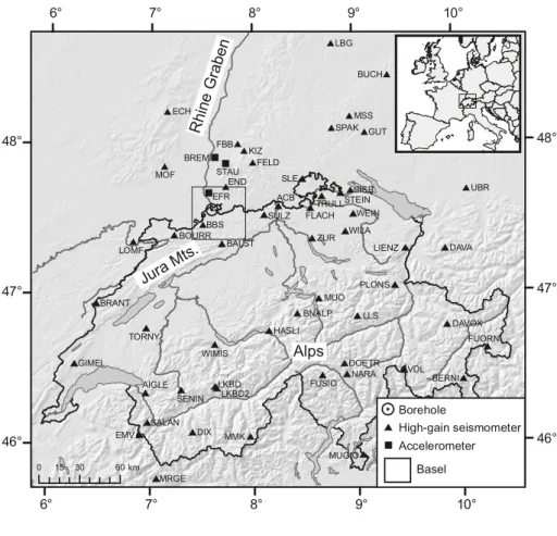
the seismic data available for the basel geothermal project and analyzed in this article were recorded by several different seismometer and accelerometer networks operated by three separate institutions, schweizerischer Erdbebendienst (sED), Landeserdbebendienst baden-Württemberg (LED) and Geo-thermal Explorers Ltd. (GEL). the locations are shown in Fig-ures 1 and 2 and comprise the following stations:

• GEL borehole sensors (in parenthesis is the depth below surface in m):

OtEr2 (2740), OtEr1 (500), JOHAN (317), HALtI (542), MAttE (553), rIEH2 (1213)

• sED high-gain seismometer-network:

bALst, bOUrr, sULZ, Acb, sLE, FLAcH, ZUr, trULL, stEIN, WILA, bNALP, HAsLI, WIMIs, tOrNY, MUO, WEIN, brANt, LKbD, LKbD2, LLs, sENIN, AIGLE, LIENZ, PLONs, FUsIO, GIMEL, DOEtr, NArA, sALAN, DIX, MMK, EMV, VDL, DAVOX, MU-GIO, FUOrN, bErNI, sENIN, DAVA, MrGE

• sED online accelerometers:

OttEr, sbAF, srHb, sbAP, sbAt sbIs sMZW sKAF sAUr

• sED offline accelerometers:

sbAE sbAJ sbAM sbEG sbIF sMZA scHc srNr • sED offline temporary accelerometers:

cHbAL, cHbbO, cHbrI, cHbMU, cHbDO, cHbPF • LED high-gain seismometer-network:

bbs, FELD, MOF, Fbb, LOMF, EcH, sIsb, sPAK, GUt, KIZ, LbG, bUcH, Ubr, END, Mss

• LED high-gain temporary seismometers: WL8, WL11, WL12

• LED accelerometers:

brEM, EFr, stAU, WEIL, WYH, LOEr, LOEs, WL2, WL7, WL9, WL10

Fig. 1. seismic stations in switzerland and south-ern Germany that supplied data used for the faultplane solutions of the induced seismicity in basel. JuraMts. Rhin eG rabe n Alps

this compilation does not include all potentially available seismic stations, but only those from which data was actually used in the analysis of the seismicity associated with the ba-sel geothermal project. the data from the borehole sensors of GEL and of the high-gain permanent seismometer network as well as of the online accelerometers of sED were available in real- or near-real-time and thus provided the basis for con-tinuous monitoring of the ongoing seismicity. the data from all other networks had to be downloaded or requested manually and then partly reformatted and integrated into the existing data files. they were thus not available for the near-real-time processing but only for a subsequent more detailed analysis, in particular for the calculation of focal mechanisms.

the borehole sensors are short-period geophones with a nat-ural frequency between 4.5 and 5 Hz and a damping coefficient of 0.21. the data was recorded at an original sampling rate of 1000 Hz, but the signals transmitted to the sED were downsam-pled to 500 Hz (OtEr1 120 Hz). In the shallower boreholes, all three orthogonal components are inclined at an angle of 54.7 de-grees, but their horizontal orientation is not known. In the deepest

monitoring well (OtEr2) the three components are mounted in the traditional way with one vertical and two horizontal, but again the horizontal orientation is not known. the high-gain network of the sED consists mainly of sts-2 broad-band seismometers and to a lesser degree of 1- and 5-second seismometers. their signals are digitized at a sampling rate of 120 Hz. the high-gain network of the LED consists of 1-second seismometers and their signals are digitized at sampling rates between 62.5 and 125 Hz. Most of the accelerometer data of the sED is available at sampling rates of 250 Hz, with some of the older off-line stations recording at sampling rates varying between 128 and 256 Hz, whereas the LED accelerometer signals are sampled at 100 Hz.

As an example, Figure 3 shows the P-phases of all 28 events, recorded by the borehole sensor at 553 m depth at station MAttE (distance 4 km) and by the broad-band seismometer at station bOUrr (distance 35 km). Note the differences in signal character visible at MAttE, which are due in part to dif-ferent focal mechanisms and in part to difdif-ferent degrees of rup-ture complexity (events 86, 108, 113, 159, 168, 170 and 174). by the time the signals arrive at station bOUrr, these differences

Fig. 2. seismic stations in basel and surround-ings, during the stimulation in December 2006 and for about six months thereafter. the darker shaded areas correspond to the city of basel and surrounding towns, while wood- and farmland are the light grey and white patches. the epicenters of the induced seismicity and the basel injection well are located immediately east of station sbAF and inbetween stations WEIL and OttEr.

FRANCE

GERMANY

have disappeared almost completely and the seismograms are dominated by path and site effects.

Focal mechanisms

Method

Focal mechanisms based on first-motion polarities were deter-mined for the 28 strongest events that occurred between

De-cember 3rd 2006 and May 6th 2007. the reliability of faultplane solutions based on first motion polarities depends strongly on correct azimuths and vertical take-off angles of the rays leav-ing the source. Normally, with data from stations at epicentral distances that are large compared to the focal depth, the un-certainty in azimuth as a function of location uncertainties can be ignored. In our case, however, the faultplane solutions are strongly constrained by several stations at epicentral distances of only a few kilometers. In order to minimize the influence of

Fig. 3. P-arrivals (ground velocity) recorded by the borehole sensor at MAttE (distance 4 km and depth 553 m) and by the broad-band seismometer at bOUrr (distance 35 km). For comparison, the signals at MAttE have been filtered with a 4th order acausal butterworth 40 Hz low-pass filter and the signals at bOUrr were convolved with the impulse response of the borehole sensor (natural frequency 5 Hz, damping 0.21). the numbers on the left side of the figure correspond to the event numbers in table 1.

-0.8 -0.6 -0.4 -0.2 0 0.2 0.4 0.6 2006 12 03 19 51 5 M 1.7 2006 12 06 22 27 2 M 2.2 2006 12 07 01 44 23 M 1.9 2006 12 08 01 49 31 M 1.9 2006 12 08 01 49 55 M 1.9 2006 12 08 03 06 19 M 2.6 2006 12 08 03 24 4 M 2.3 2006 12 08 09 01 44 M 1.8 2006 12 08 09 04 2 M 2.2 2006 12 08 11 36 29 M 2.2 2006 12 08 15 12 53 M 2.0 2006 12 08 15 29 52 M 1.8 2006 12 08 15 30 37 M 2.1 2006 12 08 15 46 56 M 2.7 2006 12 08 16 48 40 M 3.4 2006 12 08 19 26 43 M 2.3 2006 12 08 20 19 40 M 2.5 2006 12 10 06 10 39 M 2.0 2006 12 14 22 39 28 M 2.5 2006 12 19 23 50 8 M 1.8 2007 01 04 04 38 18 M 1.8 2007 01 06 07 19 53 M 3.1 2007 01 12 03 34 34 M 2.2 2007 01 15 00 02 36 M 1.9 2007 01 16 00 09 9 M 3.2 2007 02 02 03 54 28 M 3.2 2007 03 21 16 45 19 M 2.8 2007 05 06 00 34 4 M 2.3 MATTE - EHB, LP 40 Hz seconds 112 184 185 176 174 173 170 167 168 162 159 147 113 108 105 104 103 102 5 39 43 81 98 94 93 87 86 82 112 184 185 176 174 173 170 167 168 162 159 147 113 108 105 104 103 102 5 39 43 81 98 94 93 87 86 82 -0.8 -0.6 -0.4 -0.2 0 0.2 0.4 0.6 2006 12 03 19 51 10 M 1.7 2006 12 06 22 27 7 M 2.2 2006 12 07 01 44 28 M 1.9 2006 12 08 01 49 36 M 1.9 2006 12 08 01 50 0 M 1.9 2006 12 08 03 06 24 M 2.6 2006 12 08 03 24 9 M 2.3 2006 12 08 09 01 49 M 1.8 2006 12 08 09 04 7 M 2.2 2006 12 08 11 36 34 M 2.2 2006 12 08 15 12 58 M 2.0 2006 12 08 15 29 57 M 1.8 2006 12 08 15 30 42 M 2.1 2006 12 08 15 47 1 M 2.7 2006 12 08 16 48 45 M 3.4 2006 12 08 19 26 48 M 2.3 2006 12 08 20 19 46 M 2.5 2006 12 10 06 10 45 M 2.0 2006 12 14 22 39 33 M 2.5 2006 12 19 23 50 13 M 1.8 2007 01 04 04 38 23 M 1.8 2007 01 06 07 19 58 M 3.1 2007 01 12 03 34 39 M 2.2 2007 01 15 00 02 41 M 1.9 2007 01 16 00 09 14 M 3.2 2007 02 02 03 54 34 M 3.2 2007 03 21 16 45 24 M 2.8 2007 05 06 00 34 9 M 2.3 BOURR - HHZ, HP 5 Hz seconds

possibly mislocated hypocenters, we calculated azimuths and vertical take-off angles based on locations that were deter-mined relative to a well-constrained master event.

As a master event we chose the first event in table 1, which is located about 54 m from the injection well. the location of this event was determined not only from the records at the six GEL borehole sensors listed in the previous section, but also with the aid of the P-arrival time observed at a seismometer that was temporarily installed close to the casing shoe in the 5 km deep injection well during the first phase of stimulation. the differences between the calculated and observed arrival times (travel-time residuals) of the master event were then used as station corrections for all other events. this procedure takes advantage of the fact that all hypocenters are located in a restricted volume within the crystalline basement, where seis-mic velocities do not vary significantly, and of the fact that ray paths are similar for all events. consequently the remaining lo-cation errors of the hypocenters relative to each other are due to inconsistent arrival-time readings alone. As documented in more detail by Deichmann & Giardini (2009), the calculated standard deviations of the relative hypocenters determined by this method are on the order of 50 m horizontally and 70 m vertically.

to assess the influence of the location on the azimuths of the rays leaving the source, we need an estimate of the

ab-solute location accuracy of the epicenters. this is equivalent to estimating the uncertainty of the absolute location of the chosen master event as computed by GEL. A comparison of the master event locations of 183 events with the absolute lo-cations computed by GEL shows that they differ on average by 20 ± 45 m in the Ns direction and by 5 ± 65 m in the EW direction (sED 2007). Given that the location of the master event is based also on the P-arrival recorded by the geophone installed temporarily in the injection well, whereas most of the other locations are not, it is reasonable to conclude that the uncertainty of the absolute location of the master event is less than ± 65 m. Moreover, the s-phase in the seismograms of the master event, that were recorded by the temporary seismom-eter in the injection borehole, can not be clearly identified, so that the s-P time is certainly not more than about 0.01 s. this is equivalent to a maximum distance of about 80 m from the borehole, which is consistent with the 54 m determined for the absolute location by GEL. In addition, during cementation of the casing inside the well, a sequence of seismic events was in-duced by the injection of the cement into the open-hole section and the annulus between the casing and borehole wall. One of these events (2006/11/10 17 : 21 Utc) was strong enough to be recorded by the sED network (ML = 0.7). Given that the

duration of this operation was only a matter of a few hours and that consequently the injected fluid did not have enough time

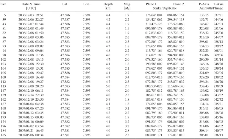
table 1. Focal mechanism parameters of the induced seismicity, based on first-motion polarities. Evn: event number in Figures 3, 6 and 7. Evn Date & time

[Utc]

Lat. Lon. Depth [km] Mag. [ML] Plane 1 Plane 2 strike/Dip/rake P-Axis t-Axis Azimuth/Plunge 5 2006/12/03 19 : 51 47.586 7.594 4.4 1.7 176/64/ 004 084/86/ 154 133/15 037/21 39 2006/12/06 22 : 27 47.587 7.593 4.2 2.2 154/42/–062 298/54/–113 152/71 044/06 43 2006/12/07 01 : 44 47.586 7.592 4.4 1.9 310/47/–123 173/52/–060 146/67 242/03 81 2006/12/08 01 : 49 47.587 7.592 4.5 1.9 096/80/–178 006/88/–010 320/08 051/06 82 2006/12/08 01 : 50 47.584 7.594 4.7 1.9 017/63/–020 116/72/–152 338/32 245/06 86 2006/12/08 03 : 06 47.585 7.595 4.1 2.6 089/78/–178 359/88/–012 313/10 044/07 87 2006/12/08 03 : 24 47.583 7.594 4.8 2.3 072/80/ 172 163/82/ 010 298/01 028/13 93 2006/12/08 09 : 02 47.583 7.596 4.2 1.8 178/65/ 007 085/84/ 155 134/13 039/22 94 2006/12/08 09 : 04 47.585 7.593 4.8 2.2 115/73/–164 020/75/–018 337/23 068/01 98 2006/12/08 11 : 36 47.584 7.596 4.6 2.2 114/82/ 180 204/90/ 008 339/06 069/06 102 2006/12/08 15 : 13 47.583 7.595 4.7 2.0 078/52/–160 335/74/–040 290/39 031/14 103 2006/12/08 15 : 30 47.585 7.594 4.1 1.8 190/58/ 009 095/82/ 148 146/16 048/28 104 2006/12/08 15 : 31 47.585 7.595 4.0 2.1 179/62/ 007 086/84/ 152 136/15 039/24 105 2006/12/08 15 : 47 47.588 7.593 4.1 2.7 097/80/–177 006/87/–010 321/09 052/05 108 2006/12/08 16 : 49 47.584 7.593 4.7 3.4 012/75/–013 105/77/–165 329/20 238/02 112 2006/12/08 19 : 27 47.582 7.596 4.7 2.3 077/58/–177 345/87/–032 296/24 036/20 113 2006/12/08 20 : 20 47.583 7.594 5.0 2.5 008/53/–028 115/68/–140 337/43 238/09 147 2006/12/10 06 : 11 47.584 7.595 4.0 2.0 182/75/ 012 089/78/ 165 136/02 045/19 159 2006/12/14 22 : 39 47.584 7.595 4.0 2.5 186/61/ 018 087/74/ 150 139/08 043/32 162 2006/12/19 23 : 50 47.584 7.595 3.9 1.8 185/61/ 018 086/74/ 150 138/08 042/32 167 2007/01/04 04 : 38 47.583 7.596 4.1 1.8 174/65/ 006 082/85/ 155 131/14 035/21 168 2007/01/06 07 : 20 47.582 7.596 4.2 3.1 091/79/–176 360/86/–011 315/11 046/05 170 2007/01/12 03 : 35 47.581 7.597 4.2 2.2 082/79/ 180 172/90/ 011 306/08 038/08 173 2007/01/15 00 : 03 47.582 7.596 4.0 1.9 182/73/ 006 090/84/ 163 137/08 045/16 174 2007/01/16 00 : 09 47.582 7.596 4.1 3.2 091/83/–176 001/86/–007 316/08 046/02 176 2007/02/02 03 : 54 47.582 7.596 4.0 3.2 089/84/–177 359/87/–006 314/06 044/02 184 2007/03/21 16 : 45 47.581 7.596 4.0 2.8 085/75/–175 354/85/–015 308/14 040/07 185 2007/05/06 00 : 34 47.581 7.596 4.0 2.3 080/80/ 171 172/81/ 010 306/01 036/13

to migrate far from the well, it is reasonable to assume that the hypocenter of this event must be located within a few tens of meters from the borehole. the location relative to the chosen master event calculated by the same procedure as described above places it 37 m west and 2 m south of the borehole. Un-fortunately the instrument in the deepest monitoring borehole (OtEr2) was not operational at that time, so the calculated standard deviation for the location of this event relative to the master event is on the order of 60 m. Nevertheless, within the attainable precision, the adopted relative location procedure based on the chosen absolute location of the master event puts this cementation event in the immediate vicinity of the bore-hole, as expected.

based on these three arguments, a standard deviation of ± 65 m for the absolute horizontal location accuracy of the master event is a reasonable estimate. combining this esti-mate with the calculated average standard deviation of the relative locations, we conclude that the absolute epicenter lo-cation accuracy for all events is on the order of 100 m. there-fore, for stations located at epicentral distances beyond 1 km, the effect of the epicenter location uncertainty on the azimuth values used for the faultplane solutions is insignificant in most cases.

Vertical take-off angles are a function of epicentral dis-tance, focal depth and P-wave velocities between source and stations. Given the close epicentral distances of many stations that recorded the induced seismicity of basel and the heterog-enous velocity structure beneath each station, take-off angles calculated by standard hypocenter-location software are not sufficiently reliable. to account for lateral variations of the near-surface structure, all surface-stations were assigned to one of four typical velocity models (Figure 4):

• Model 1: cHbAL cHbbO sbIF srNr EFr

• Model 2: OttEr sbAF sbAP sbAt sbIs srHb cHbDO cHbPF sbAE sbAJ sbAM WL8 WL11 WL12 WL2 WL7 WL9 WL10 LOEr LOEs WEIL

• Model 3: cHbMU cHbrI cHbFr

• Model 4: sKAF sMZW sAUr sbEG sMZA scHc WYH bbs

these models were obtained by grouping the individual sta-tion models used by ripperger et al. (2009) for calculating synthetic ground motions, based on a detailed structural model constructed for the basel area by Fäh & Huggenberger (2006). the borehole stations were assigned to one of three velocity models, derived from Model 2 shown in Figure 4: one for the shallower sensors (300–500 m), one for rIEH2 (1213 m) and one for OtEr2 (2740 m).

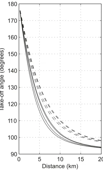
A ray-trace computer code modified after Gebrande (1976) was used to calculate epicentral distances for a range of take-off angles in increments of 1 degree for two focal depths (4 and 5 km below the earth’s surface) and for each of the seven models. Figure 5 shows how the take-off angles for the surface stations vary with epicentral distance for the four models and

for the two focal depths of 4 and 5 km. From this Figure we see that an error of 1 km in focal depth can easily lead to a take-off-angle error of 10 degrees. A similar variation in take-off take-off-angle for a given focal depth can also occur at epicentral distances be-low 5 km as a consequence of differences in the velocity model. to obtain reliable faultplane solutions based on observations at close epicentral distances, it is important to take these effects into account.

For our case, the corrected take-off angles for all stations at epicentral distances less than 16 km and for the focal depth determined by the master-event relocation for each event were calculated by interpolating between the values of the two fo-cal-depth extremes shown in Figure 5 using the appropriate velocity model.

Fig. 4. P-wave velocities (km/s) used for calculating vertical take-off angles to the surface stations. beyond a depth of 3 km, velocity was assumed to be 5.95 km/s in all models.

1

2

3

4

3

2

1

0

Depth

(km

)

Model Number

5.6

0.9

5.6

0.9

5.6

0.9

5.6

0.9

5.2

5.2

5.2

5.2

4.2

4.2

4.2

4.2

3.4

3.4

3.4

1.8

1.8

Results

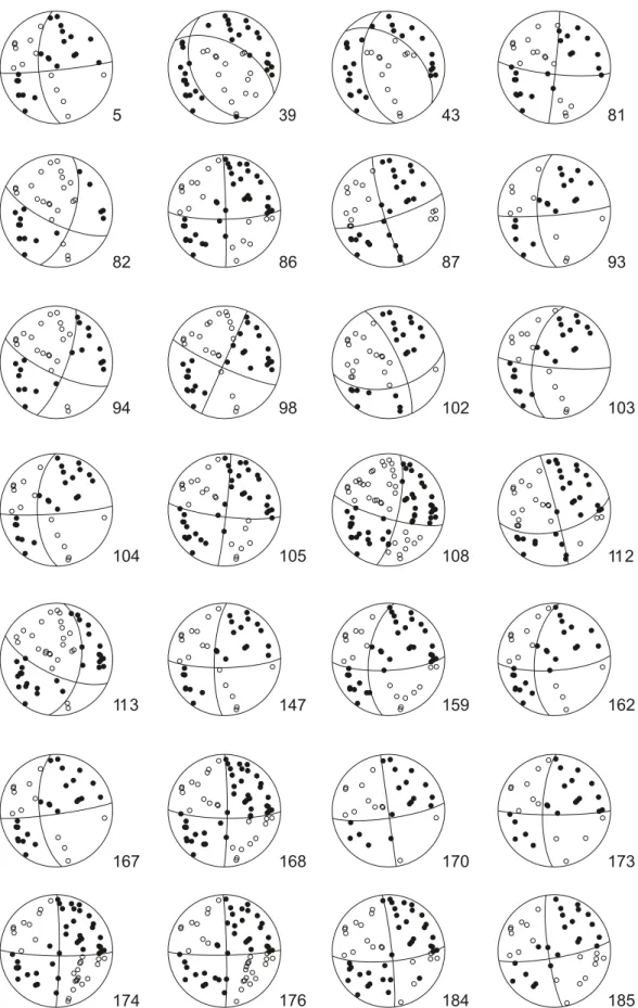
the stereographic plots with the individual first motions are displayed in Figure 6 and the corresponding parameters are listed in table 1. Given the large number of temporary stations installed in the epicentral area, the focal sphere is well sampled even for events as small as ML 1.7, and the resulting

mecha-nisms are well constrained. Nevertheless, in some cases discrep-ant first-motion polarities could not be avoided. In fitting the observed polarities it was always attempted to define the nodal planes in such a way as to maximise the number of matching polarities. Most of the discrepancies are observed at stations OttEr, OtEr1 and OtEr2. As argued in the previous sec-tion, despite the fact that these stations are located at short

epicentral distances, it is highly unlikely that the inconsistent polarities are due to location errors. Whether this is evidence for non-double-couple components of the focal mechanisms is discussed in more detail by Deichmann & Giardini (2009). However, the solutions presented here can be regarded as the best double-couple solutions (shear dislocations) and are thus comparable to previously observed focal mechanisms of natu-rally occurring earthquakes.

Discussion

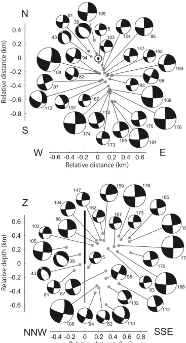
Figure 7 shows the resulting focal mechanisms on an epicen-ter map and a depth cross-section with the masepicen-ter-event relo-cations. A polar histogram with the strike of all nodal planes and a stereographic plot with the orientation of all P- and t-axes is shown in Figure 8. According to the criteria of the World stress Map Project (Zoback 1992), of the 28 faultplane solutions, two are normal faulting mechanisms and one is a strike-slip mechanism with a strong normal component. All others are typical strike-slip mechanisms with mostly Ns and EW striking nodal planes. As a consequence, the t-axes are all nearly horizontal and oriented in a NE or sW direction (mean azimuth 46 ± 11 degrees) and the P-axes of the strike-slip events point in a NW or sE direction (mean azimuth 138 ± 13 degrees).

Given the relatively small scatter of the orientations of the P- and t-axes, a formal stress inversion would not be particu-larly well constrained. Nevertheless it is instructive to compare the orientations of the P- and t-axes as well as the strike of the nodal planes of the induced seismicity with the stress field de-duced from the naturally occurring earthquakes in the region of basel and with the in situ stress observations in the borehole itself. As documented in earlier studies, the focal mechanisms available until 1999 for the southern rhinegraben, the black Forest and northern switzerland south of basel, are dominated by strike-slip and normal faulting mechanisms (Plenefisch & bonjer 1997, Evans & roth 1998, Kastrup et al. 2004). A few more recent events documented in the annual reports of the swiss seismological service are of the same type (Deichmann et al. 2000, baer et al. 2001, Deichmann et al. 2002, Deichmann et al. 2004, baer et al. 2005).

the average value for the direction of the regional maxi-mum compressive horizontal stress, SHmax, calculated by

Kas-trup et al. (2004) from the focal mechanisms in the southern rhinegraben region and in the central part of northern swit-zerland, using two different inversion methods, is about 144 degrees. this value is identical to the average local SHmax in the

crystalline basement derived from measurements in the 5 km deep basel borehole by Valley & Evans (2006, 2009).

Whether the focal mechanisms are evidence for rupture having occurred on faults that are optimally oriented with re-spect to the ambient tectonic stress depends on which of the two nodal planes actually corresponds to the active faultplane. based on high-precision relative locations by Asanuma et al. (2007) and Kumano et al. (2007) of hypocenters belonging

Fig. 5. Vertical take-off angles as a function of epicentral distance to the sur-face stations for a focal depth of 4 km (continuous curves) and 5 km (dashed curves). For each focal depth, the bottom curve corresponds to model number 1 and the top curve to model number 4 (see Figure 4).

0

5

10

15

20

90

100

110

120

130

140

150

160

170

180

Distance (km)

Take-of

fangle

(degrees)

Fig. 6. Fault-plane solutions based on first-motion polarities. All stereographs are lower hemisphere, equal area projections; solid circles correspond to compres-sive first motion (up) and empty circles to dilatational first motion (down). the number next to each stereograph corresponds to the event numbers in table 1.

184

185

174

173

170

168

162

167

159

147

113

112

108

105

104

103

102

98

93

87

86

82

81

43

39

5

176

94

to families of similar events, Häring et al. (2008) suggest that both the more favourably oriented N–s and the less favourably E–W oriented nodal planes were active. From a similar analy-sis of a sub-cluster that includes the ML 3.4 mainshock (event

No. 108), as well as events no. 82 and 94 (Figure 6), Deichmann

& Giardini (2009) conclude that this mainshock occurred on the WNW–EsE striking faultplane, which is indeed optimally oriented with respect to the principal stress axes. Note that the WNW–EsE alignement of these three events is visible even at the scale of the epicenter map in Figure 7.

Conclusions

the 28 faultplane solutions documented in this article are an important addition to the focal mechanism data available in the basel region. In fact, the hypocenters of most of the events for which focal mechanisms have been known previously are located at depths below 10 or even 20 km, and the shallowest of these is 7 km deep (bonjer 1997). thus the induced seismic-ity below basel, which is located at very well-constrained fo-cal depths between 4 and 5 km, samples the crust in a depth interval where data has been lacking in the past. In addition, it represents a rare case in which focal mechanisms and indepen-dent in situ stress observations are available for the exact same crustal volume.

Acknowledgements

this study would not have been possible without the cooperation of Geother-mal Explorers Ltd., who gave us realtime access to the data of their borehole sensors, and part of this work was done with financial support by Geopower basel AG; both contributions are gratefully acknowledged. Moreover, part of this work constitutes a contribution to the interdisciplinary research proj-ect GEOtHErM, funded by the competence center of Environment and sustainability (ccEs) of EtH (http://www.cces.ethz.ch/projects/nature/geo-therm/). We are particularly endebted to W. brüstle and s. stange of the Lan-deserdbebendienst baden-Württemberg in Freiburg for sending us all their waveform data, which was crucial for much of this study. thanks are due to s. Wöhlbier, who contributed to this article with several figures, as well as to c. bärlocher and his colleagues of the electronics lab of sED and to M. baer for their efforts in establishing and maintaining access to the data of the bore-hole stations in basel. Keith Evans carefully reviewed a first version of the manuscript and contributed several suggestions for improvements. Helpful re-views of the submitted manuscript by thomas Plenefisch and thomas Fischer are also gratefully acknowledged.

Fig. 7. Epicenter map (top) and depth cross-section (bottom) with master-event locations and focal mechanisms. In both figures, the faultplane solu-tions correspond to lower-hemisphere, equal area projecsolu-tions as seen from above. In the map, the location of the basel geothermal well is indicated by the circle with the black dot, whereas in the cross-section, the vertical line marks the cased (thick) and open (thin) section of the borehole. the size of each stereograph is proportional to magnitude (1.7 ≤ ML ≤ 3.4) and the numbers correspond to the event numbers in table 1.

-0.4 -0.2 0 0.2 0.4 0.6 0.8 -0.6 -0.4 -0.2 0 0.2 0.4 0.6

SSE

NNW

Z

W

E

S

N

Fig. 8. symmetric polar histogram of the strike of the focal mechanism nodal planes and stereographic equal area plots of the P-axes (empty circles) and the t-axes (black circles) for the 28 induced events. the arrows point in the direction of the maximum horizontal compressive stress derived from bore-hole observations in the crystalline basement down to 5 km depth by Valley & Evans (2006, 2009).

rEFErENcEs

Asanuma, H., Kumano, Y., Hotta, A., schanz, U., Niitsuma, H., Häring, M., 2007: Analysis of microseismic events from a stimulation at basel, swit-zerland. Grc transactions, 31, 265–269.

baer, M., Deichmann, N., braunmiller, J., ballarin Dolfin, D., bay, F., bernardi, F., Delouis, b., Fäh, D., Gerstenberger, M., Giardini, D., Hu-ber, s., Kastrup, U., Kind, F., Kradolfer, U., Maraini, s., Mattle, b., schler, t., salichon, J., sellami, s., steimen, s., Wiemer, s. 2001: Earthquakes in switzerland and surrounding regions during 2000. Eclogae Geologicae Helvetiae 94/2, 253–264.

baer, M., Deichmann, N., braunmiller, J., Husen, s., Fäh, D., Giardini, D., Kästli, P., Kradolfer, U., Wiemer, s. 2005: Earthquakes in switzerland and surrounding regions during 2004. Eclogae Geologicae Helvetiae – swiss Journal of Geosciences 98/3, 407–418. DOI: 10.1007/s00015–005–1168–3. bonjer, K.-P. 1997: seismicity pattern and style of seismic faulting at the

east-ern borderfault of the southeast-ern rhine Graben. tectonophysics 275, 41–69, 1997.

Deichmann, N., ballarin Dolfin, D. & Kastrup, U. 2000: seismizität der Nord- und Zentralschweiz. Nagra technischer bericht, Ntb 00–05, Nagra, Wet-tingen.

Deichmann, N., baer, M., braunmiller, J., ballarin Dolfin, D., bay, F., bernardi, F., Delouis, b., Fäh, D., Gerstenberger, M., Giardini, D., Huber, s., Kra-dolfer, U., Maraini, s., Oprsal, I., schibler, r., schler, t., sellami, s., stei-men, s., Wiemer, s., Wössner, J., Wyss, A. 2002: Earthquakes in switzer-land and surrounding regions during 2001. Eclogae Geologicae Helvetiae – swiss Journal of Geosciences 95/2, 249–261.

Deichmann, N., baer, M., braunmiller, J., cornou, c., Fäh, D., Giardini, D., Gisler, M., Huber, s., Husen, s., Kästli, P., Kradolfer, U., Mai, M., Maraini, s., Oprsal, I., schler, t., schorlemmer, D., Wiemer, s., Wössner, J., Wyss, A. 2004: Earthquakes in switzerland and surrounding regions during 2003. Eclogae Geologicae Helvetiae – swiss Journal of Geosciences 97/3, 447–458.

Deichmann, N. & Giardini, D. 2009: Earthquakes induced by the stimulation of an enhanced geothermal system below basel (switzerland). seismo-logical research Letters 80/5, 784–798, doi:10.1785/gssrl.80.5.784. Dyer, b.c., schanz, U., Ladner, F., Häring, M.O., spillmann, t. 2008:

Microseis-mic imaging of a geothermal reservoir stimulation. the Leading Edge 27, 856–869.

Evans, K.F. & roth P. 1998: the state of stress in northern switzerland inferred from earthquake seismological data and in-situ stress measurements. re-port prepared for the Deep Heat Mining (DHM) Project basel on behalf of Geothermal Explorers Ltd., Pratteln, switzerland, 26 pp.

Fäh, D. & Huggenberger, P. 2006. INtErrEG III Erdbebenmikrozonierung am südlichen Oberrhein, Zusammenfassung für das Projektgebiet in der schweiz, cD and report (in german; available from the authors), swiss seis-mological service, EtH Zurich and Kantonsgeologie, University of basel.

Gebrande, H. 1976: A seismic ray-tracing method for two-dimensional inho-mogeneous media. In: Explosion seismology in central Europe. ed. by Giese P., Prodehl, c., stein, A.; springer, 162–167.

Häring, M.O., schanz, U., Ladner, F., Dyer, b.c. 2008: characterization of the basel 1 enhanced geothermal system. Geothermics 37, 469–495, doi:10.1016/j.geothermics.2008.06.002.

Kastrup, U., Zoback M.-L., Deichmann, N., Evans, K., Giardini, D., Michael, A. J. 2004: stress field variations in the swiss Alps and the northern Alpine foreland derived from inversion of fault plane solutions. Journal of Geo-physical research 109/b1, doi:10.1029/2003Jb002550b01402.

Kraft, t., Mai, P.M., Wiemer, s., Deichmann, N., ripperger, J., Kästli, P., bach-mann, c., Fäh, D., Wössner, J., and Giardini, D. (2009): Mitigating risk for Enhanced Geothermal systems in Urban Areas. EOs transactions American Geophysical Union, 90/32, 273–274.

Kumano, Y., Asanuma, H., Hotta, A., Niitsuma, H., schanz, U., Häring, M., 2007: reservoir structure delineation by microseismic multiplet analysis at basel, switzerland, 2006. Paper presented at the 77th sEG meeting, san Antonio, tX, UsA, Extended Abstracts, 1271–1276.

Plenefisch, t. & bonjer, K.-P. 1997: the stress field in the rhinegraben area inferred from earthquake focal mechanisms and estimation of frictional parameters. tectonophysics 275, 71–97.

ripperger, J., Kästli, P., Fäh, D., Giardini, D. 2009: Ground motion and macro-seismic intensities of a macro-seismic event related to geothermal reservoir stim-ulation below the city of basel – observations and modelling. Geophysical Journal International, DOI: 10.1111/j.1365-246X.2009.04374.X.

sED 2007: Evaluation of the induced seismicity in basel 2006/2007 – loca-tions, magnitudes, focal mechanisms, statistical forecasts and earthquake scenarios. report of the swiss seismological service to Geopower basel AG, December 2007.

Ustaszewski, K. & schmid, s.M. 2007: Latest Pliocene to recent thick-skinned tectonics at the Upper rhine Graben – Jura Mountains junction. swiss Journal of Geosciences 100, 293–312.

Valley, b. & Evans, K.F. 2006: stress orientation at the basel geothermal site from wellbore failure analysis in bs1. report to Geopower basel AG for swiss Deep Heat Mining Project basel. EtH report Nr.: EtH 3465/56. Ingenieurgeologie EtH Zürich, switzerland, 29 pp.

Valley, b. & Evans, K.F. 2009: stress orientation to 5 km depth in the basement below basel (switzerland) from borehole failure analysis. swiss Journal of Geosciences, DOI 10.1007/s00015-009-1335-z.

Zoback, M.L. 1992: First- and second Order Patterns of stress in the Litho-sphere: the World stress Map Project, Journal of Geophysical research 97/b8, 11703–11711.

Manuscript received January 12, 2009 revision accepted July 8, 2009

Published Online first November 30, 2009 Editorial Handling: A. Hirt & s. bucher