HAL Id: insu-01175648
https://hal-insu.archives-ouvertes.fr/insu-01175648
Submitted on 29 Feb 2016
HAL is a multi-disciplinary open access
archive for the deposit and dissemination of
sci-entific research documents, whether they are
pub-lished or not. The documents may come from
teaching and research institutions in France or
abroad, or from public or private research centers.
L’archive ouverte pluridisciplinaire HAL, est
destinée au dépôt et à la diffusion de documents
scientifiques de niveau recherche, publiés ou non,
émanant des établissements d’enseignement et de
recherche français ou étrangers, des laboratoires
publics ou privés.
emissions in the summertime in northern Norway: from
the local to the regional scale
Louis Marelle, Jennie L. Thomas, Jean-Christophe Raut, Kathy S. Law,
Jukka-Pekka Jalkanen, Lasse Johansson, Anke Roiger, Hans Schlager, Jin
Kim, Anja Reiter, et al.
To cite this version:
Louis Marelle, Jennie L. Thomas, Jean-Christophe Raut, Kathy S. Law, Jukka-Pekka Jalkanen, et al..
Air quality and radiative impacts of Arctic shipping emissions in the summertime in northern Norway:
from the local to the regional scale. Atmospheric Chemistry and Physics, European Geosciences Union,
2016, 16 (4), pp.2359-2379. �10.5194/acp-16-2359-2016�. �insu-01175648�
www.atmos-chem-phys.net/16/2359/2016/ doi:10.5194/acp-16-2359-2016
© Author(s) 2016. CC Attribution 3.0 License.
Air quality and radiative impacts of Arctic shipping emissions
in the summertime in northern Norway: from the local to
the regional scale
Louis Marelle1,2, Jennie L. Thomas1, Jean-Christophe Raut1, Kathy S. Law1, Jukka-Pekka Jalkanen3, Lasse Johansson3, Anke Roiger4, Hans Schlager4, Jin Kim4, Anja Reiter4, and Bernadett Weinzierl4,5
1LATMOS/IPSL, UPMC Univ. Paris 06 Sorbonne Universités, UVSQ, CNRS, Paris, France 2TOTAL S.A, Direction Scientifique, Tour Michelet, 92069 Paris La Defense, France 3Finnish Meteorological Institute, Helsinki, Finland
4Institut für Physik der Atmosphäre, Deutsches Zentrum für Luft- und Raumfahrt (DLR), Oberpfaffenhofen, Germany 5Ludwig Maximilians Universität (LMU), Meteorologisches Institut, 80333, München, Germany
Correspondence to: Louis Marelle (louis.marelle@latmos.ipsl.fr) and Jennie L. Thomas (jennie.thomas@latmos.ipsl.fr)
Received: 15 April 2015 – Published in Atmos. Chem. Phys. Discuss.: 7 July 2015 Revised: 12 January 2016 – Accepted: 1 February 2016 – Published: 29 February 2016
Abstract. In this study, we quantify the impacts of
ship-ping pollution on air quality and shortwave radiative ef-fect in northern Norway, using WRF-Chem (Weather Re-search and Forecasting with chemistry) simulations com-bined with high-resolution, real-time STEAM2 (Ship Traf-fic Emissions Assessment Model version 2) shipping emis-sions. STEAM2 emissions are evaluated using airborne mea-surements from the ACCESS (Arctic Climate Change, Econ-omy and Society) aircraft campaign, which was conducted in the summer 2012, in two ways. First, emissions of ni-trogen oxides (NOx) and sulfur dioxide (SO2) are derived
for specific ships by combining in situ measurements in ship plumes and FLEXPART-WRF plume dispersion modeling, and these values are compared to STEAM2 emissions for the same ships. Second, regional WRF-Chem runs with and without STEAM2 ship emissions are performed at two differ-ent resolutions, 3 km × 3 km and 15 km × 15 km, and evalu-ated against measurements along flight tracks and average campaign profiles in the marine boundary layer and lower troposphere. These comparisons show that differences be-tween STEAM2 emissions and calculated emissions can be quite large (−57 to +148 %) for individual ships, but that WRF-Chem simulations using STEAM2 emissions repro-duce well the average NOx, SO2 and O3 measured during
ACCESS flights. The same WRF-Chem simulations show that the magnitude of NOx and ozone (O3) production from
ship emissions at the surface is not very sensitive (< 5 %) to the horizontal grid resolution (15 or 3 km), while sur-face PM10 particulate matter enhancements due to ships are
moderately sensitive (15 %) to resolution. The 15 km reso-lution WRF-Chem simulations are used to estimate the re-gional impacts of shipping pollution in northern Norway. Our results indicate that ship emissions are an important source of pollution along the Norwegian coast, enhancing 15-day-averaged surface concentrations of NOx (∼ +80 %),
SO2(∼ +80 %), O3(∼ +5 %), black carbon (∼ +40 %), and
PM2.5(∼ +10 %). The residence time of black carbon
origi-nating from shipping emissions is 1.4 days. Over the same 15-day period, ship emissions in northern Norway have a global shortwave (direct + semi-direct + indirect) radiative effect of −9.3 m W m−2.
1 Introduction
Shipping is an important source of air pollutants and their precursors, including carbon monoxide (CO), nitrogen ox-ides (NOx), sulfur dioxide (SO2), volatile organic
com-pounds (VOCs) as well as organic carbon (OC) and black carbon (BC) aerosols (Corbett and Fischbeck, 1997; Corbett and Köhler, 2003). It is well known that shipping emissions have an important influence on air quality in coastal regions,
often enhancing ozone (O3) and increasing aerosol
concen-trations (e.g., Endresen et al., 2003). Corbett et al. (2007) and Winebrake et al. (2009) showed that aerosol pollution from ships might be linked to cardiopulmonary and lung dis-eases globally. Because of their negative impacts, shipping emissions are increasingly subjected to environmental regu-lations. The International Maritime Organization (IMO) has designated several regions as Sulfur Emission Control Areas (SECAs; including the North Sea and Baltic Sea in Europe), where low sulfur fuels must be utilized to minimize the air quality impacts of shipping on particulate matter (PM) lev-els. The sulfur content in ship fuels in SECAs was limited to 1 % by mass in 2010, decreasing to 0.1 % in 2015, while the global average is 2.4 % (IMO, 2010). Less strict sulfur emis-sion controls (0.5 %) will also be implemented worldwide, at the latest in 2025, depending on current negotiations. Ships produced or heavily modified recently must also comply to lower NOx emissions factors limits, reducing emission
fac-tors (in g kWh−1) by approximately −10 % (after 2000) and another −15 % (after 2011) compared to ships built before year 2000 (IMO, 2010). Jonson et al. (2015) showed that the creation of the North Sea and Baltic Sea SECAs was effective in reducing current pollution levels in Europe, and that fur-ther NOxand sulfur emission controls in these regions could
help to achieve strong health benefits by 2030 by reducing PM levels.
In addition to its impacts on air quality, maritime traf-fic already contributes to climate change, by increasing the concentrations of greenhouse gases (CO2, O3) and aerosols
(SO4, OC, BC) (Capaldo et al., 1999; Endresen et al., 2003).
The current radiative forcing of shipping emissions is neg-ative and is dominated by the cooling influence of sulfate aerosols formed from SO2emissions (Eyring et al., 2010).
However, due to the long lifetime of CO2compared to
sul-fate, shipping emissions warm the climate in the long term (after 350 years; Fuglestvedt et al., 2009). In the future, global shipping emissions of SO2are expected to decrease
due to IMO regulations, while global CO2emissions from
shipping will continue to grow due to increased traffic. This combination is expected to cause warming relative to the present day (Fuglestvedt et al., 2009; Dalsøren et al., 2013).
In addition to their global impacts, shipping emissions are of particular concern in the Arctic, where they are projected to increase in the future as sea ice declines (for details of fu-ture sea ice, e.g., Stroeve et al., 2011). Decreased summer sea ice, associated with warmer temperatures, is progressively opening the Arctic region to transit shipping, and projec-tions indicate that new trans-Arctic shipping routes should be available by mid-century (Smith and Stephenson, 2013). Other shipping activities are also predicted to increase, in-cluding shipping associated with oil and gas extraction (Pe-ters et al., 2011). Sightseeing cruises have increased signif-icantly during the last decades (Eckhardt et al., 2013), al-though it is uncertain whether or not this trend will continue. Future Arctic shipping is expected to have important impacts
on air quality in a now relatively pristine region (e.g., Granier et al., 2006), and will influence both Arctic and global cli-mate (Dalsøren et al., 2013; Lund et al., 2012). In addition, it has recently been shown that routing international mar-itime traffic through the Arctic, as opposed to traditional routes through the Suez and Panama canals, will result in warming in the coming century and cooling on the long term (150 years). This is due to the opposite sign of impacts due to reduced SO2linked to IMO regulations and reduced CO2
and O3associated with fuel savings from using these shorter
Arctic routes (Fuglestvedt et al., 2014). In addition, sulfate is predicted to cause a weaker cooling effect for the northern routes (Fuglestvedt et al., 2014).
Although maritime traffic is relatively minor at present in the Arctic compared to global shipping, even a small number of ships can significantly degrade air quality in regions where other anthropogenic emissions are low (Aliabadi et al., 2015; Eckhardt et al., 2013). Dalsøren et al. (2007) and Ødemark et al. (2012) have shown that shipping emissions also influ-ence air quality and climate along the Norwegian and Rus-sian coasts, where current Arctic ship traffic is the largest. Both studies (for years 2000 and 2004) were based on emis-sion data sets constructed using ship activity data from the AMVER (Automated Mutual-Assistance VEssel Rescue sys-tem) and COADS (Comprehensive Ocean–Atmosphere Data Set) data sets. However, the AMVER data set is biased to-wards larger vessels (> 20 000 t) and cargo ships (Endresen et al., 2003), and both data sets have limited coverage in Eu-rope (Miola and Ciuffo, 2011). More recently, ship emissions using new approaches have been developed that use ship ac-tivity data more representative of European maritime traffic, based on the AIS (Automatic Identification System) ship po-sitioning system. These include the STEAM2 (Ship Traffic Emissions Assessment Model version 2) shipping emissions, described in Jalkanen et al. (2012) and an Arctic-wide emis-sion inventory described in Winther et al. (2014). To date, quantifying the impacts of Arctic shipping on air quality and climate has also been largely based on global model studies, which are limited in horizontal resolution. In addition, there have not been specific field measurements focused on Arc-tic shipping that could be used to study the local influence of shipping emissions in the European Arctic and to validate model predicted air quality impacts.
In this study, we aim to quantify the impacts of shipping along the Norwegian coast in July 2012, using airborne mea-surements from the ACCESS (Arctic Climate Change, Econ-omy and Society) aircraft campaign (Roiger et al., 2015). This campaign (Sect. 2) took place in summer 2012 in north-ern Norway, and was primarily dedicated to the study of lo-cal pollution sources in the Arctic, including pollution origi-nating from shipping. ACCESS measurements are combined with two modeling approaches, described in Sect. 3. First, we use the Weather Research and Forecasting (WRF) model to drive the Lagrangian particle dispersion model FLEXPART-WRF run in forward mode to predict the dispersion of ship
emissions. FLEXPART-WRF results are used in combina-tion with ACCESS aircraft measurements in Sect. 4 to derive emissions of NOx and SO2for specific ships sampled
dur-ing ACCESS. The derived emissions are compared to emis-sions from the STEAM2 model for the same ships. Then, we perform simulations with the WRF-Chem model, including STEAM2 ship emissions, in order to examine in Sect. 5 the local (i.e., at the plume scale) and regional impacts of ship-ping pollution on air quality and shortwave radiative effects along the coast of northern Norway.
2 The ACCESS aircraft campaign
The ACCESS aircraft campaign took place in July 2012 from Andenes, Norway (69.3◦N, 16.1◦W); it included
character-ization of pollution originating from shipping (four flights) as well as other local Arctic pollution sources (details are available in the ACCESS campaign overview paper; Roiger et al., 2015). The aircraft (DLR Falcon 20) payload in-cluded a wide range of instruments measuring meteorolog-ical variables and trace gases, described in detail by Roiger et al. (2015). Briefly, O3 was measured by UV
(ultravio-let) absorption (5 % precision, 0.2 Hz), nitrogen oxide (NO), and nitrogen dioxide (NO2) by chemiluminescence and
pho-tolytic conversion (10 % precision for NO, 15 % for NO2;
1 Hz), and SO2 by chemical ionization ion trap mass
spec-trometry (20 % precision; 0.3 to 0.5 Hz). Aerosol size dis-tributions between 60 nm and 1 µm were measured using a Ultra-High Sensitivity Aerosol Spectrometer Airborne.
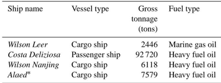
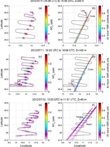
The four flights focused on shipping pollution took place on 11, 12, 19, and 25 July 2012 and are shown in Fig. 1a (details on the 11 and 12 July 2012 flights shown in Fig. 1b). The three flights on 11, 12, and 25 July 2012 sampled pollu-tion from specific ships (referred to as single-plume flights). During these flights, the research aircraft repeatedly sam-pled relatively fresh emissions from one or more ships dur-ing flight legs at constant altitudes, at several distances from the emission source, and in some cases at different altitudes. In this study, measurements from these single-plume flights are used in combination with ship plume dispersion simu-lations (described in Sects. 3.1 and 4.1) to estimate emis-sions from individual ships. This method relies on knowing the precise locations of the ships during sampling. Because those locations are not known for the ship emissions sam-pled on 25 July 2012 flight, emissions are only calculated for the three ships targeted during the 11 and 12 July flights (the Costa Deliziosa, Wilson Leer, and Wilson Nanjing), and for an additional ship (the Alaed) sampled during the 12 July flight, whose location could be retrieved from the STEAM2 shipping emission inventory (presented in Sect. 3.3). Table 1 gives more information about these four ships, one large cruise ship and three cargo ships. On 11 and 12 July 2012, the research aircraft sampled fresh ship emissions within the boundary layer, during flight legs at low altitudes (< 200 m).
Table 1. Description of the ships sampled during the ACCESS
flights on 11 and 12 July 2012.
Ship name Vessel type Gross Fuel type tonnage
(tons)
Wilson Leer Cargo ship 2446 Marine gas oil
Costa Deliziosa Passenger ship 92 720 Heavy fuel oil
Wilson Nanjing Cargo ship 6118 Heavy fuel oil
Alaed∗ Cargo ship 7579 Heavy fuel oil
∗Ship present in STEAM2, not targeted during the campaign.
Fresh ship emissions were sampled less than 4 h after emis-sion. In addition to the single-plume flights, the 19 July 2012 ACCESS flight targeted aged ship emissions in the marine boundary layer near Trondheim. Data collected during the 11 and 12 July 2012 flights are used to derive emissions from operating ships (Sect. 4), and data from the four flights (11, 12, 19, and 25 July 2012) are used to evaluate regional chemical transport simulations investigating the impacts of shipping in northern Norway (Sect. 5). Other flights from the ACCESS campaign were not used in this study because their flight objectives biased the measurements towards other emissions sources (e.g., oil platforms in the Norwegian Sea) or because they included limited sampling in the boundary layer (flights north to Svalbard and into the Arctic free tropo-sphere; Roiger et al., 2015).
3 Modeling tools
3.1 FLEXPART-WRF and WRF
Plume dispersion simulations are performed with FLEXPART-WRF for the four ships presented in Ta-ble 1, in order to estimate their emissions of NOx and
SO2. FLEXPART-WRF (Brioude et al., 2013) is a version
of the Lagrangian particle dispersion model FLEXPART (Stohl et al., 2005), driven by meteorological fields from the mesoscale weather forecasting model WRF (Skamarock et al., 2008). In order to drive FLEXPART-WRF, a meteoro-logical simulation was performed with WRF version 3.5.1, from 4 to 25 July 2012, over the domain presented in Fig. 1a. The domain (15 km × 15 km horizontal resolution with 65 vertical eta levels between the surface and 50 hPa) covers most of northern Norway (∼ 62 to 75◦N) and includes the
region of all ACCESS flights focused on ship emissions. The first week of the simulation (4 to 10 July included) is used for model spin-up. WRF options and parameterizations used in these simulations are shown in Table 2. Meteorological initial and boundary conditions are obtained from the FNL (abbreviation for “final”) analysis from NCEP (National Centers for Environmental Prediction). The simulation is also nudged to FNL winds, temperature, and humidity every
Figure 1. WRF and WRF-Chem domain (a) outer domains used for the MET, CTRL, and NOSHIP runs. ACCESS flight tracks during 11, 12,
19a (a – denotes that this was the first flight that occurred on this day, flight 19b – the second flight was dedicated to hydrocarbon extraction facilities) and 25 July 2012 flights are shown in color. (b) Inner domain used for the CTRL3 and NOSHIPS3 simulations, with the tracks of the four ships sampled during the 11 and 12 July 2012 flights (routes extracted from the STEAM2 inventory).
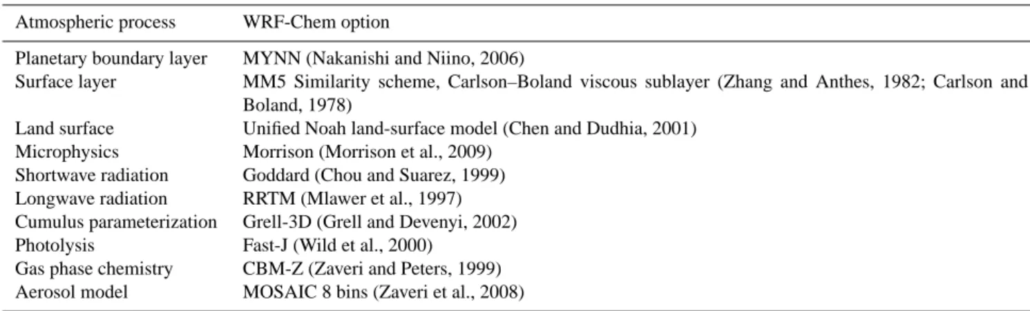
Table 2. Parameterizations and options used for the WRF and WRF-Chem simulations.
Atmospheric process WRF-Chem option
Planetary boundary layer MYNN (Nakanishi and Niino, 2006)
Surface layer MM5 Similarity scheme, Carlson–Boland viscous sublayer (Zhang and Anthes, 1982; Carlson and Boland, 1978)
Land surface Unified Noah land-surface model (Chen and Dudhia, 2001) Microphysics Morrison (Morrison et al., 2009)
Shortwave radiation Goddard (Chou and Suarez, 1999) Longwave radiation RRTM (Mlawer et al., 1997) Cumulus parameterization Grell-3D (Grell and Devenyi, 2002) Photolysis Fast-J (Wild et al., 2000)
Gas phase chemistry CBM-Z (Zaveri and Peters, 1999) Aerosol model MOSAIC 8 bins (Zaveri et al., 2008)
6 h. This WRF meteorological simulation is referred to as the MET simulation.
Ship emissions are represented in the FLEXPART-WRF plume dispersion simulations as moving 2 m × 2 m × 2 m box sources, whose locations are updated every 10 s along the ship trajectory (routes shown in Fig. 1b). In all, 1000 particles are released every 10 s into these volume sources, representing a constant emission flux with time of an inert tracer. During the ACCESS flights, targeted ships were mov-ing at relatively constant speeds durmov-ing the ∼ 3 h of the flight, meaning that fuel consumption and emission fluxes are likely to be constant during the flights if environmental conditions (wind speed, waves, and currents) were not varying strongly. FLEXPART-WRF takes into account a simple exponential decay using a prescribed lifetime. In our case, the lifetime of NOx relative to reaction with OH was estimated using
results from WRF-Chem simulations presented in Sect. 3.2. Specifically, we use OH concentrations, temperature, and air
density from the CTRL3 simulation (Sects. 3.2 and 5.1). The NOxlifetime was estimated to be 12 h on 11 July and 5 h on
12 July. The SO2lifetime was not taken into account,
consis-tent with the findings of Lee et al. (2011), who reported a life-time of ∼ 20 h over the mid-Atlantic during summer, which is significantly longer than the ages of plumes measured dur-ing ACCESS. The FLEXPART-WRF output consists of par-ticle positions, each associated with a pollutant mass; these particles are mapped onto a 3-D output grid (600 m × 600 m, with 18 vertical levels between 0 and 1500 m a.s.l.) to derive fields of volume mixing ratios every minute. Since emissions are assumed to be constant with time, and since our simu-lations only take into account transport processes depending linearly on concentrations, the intensity of these mixing ratio fields also depend linearly on the emission strength chosen for the simulation. Therefore, the model results can be scaled a posteriori to represent any constant emission flux value.
Ship emissions can continue to rise after leaving the ex-haust, due to their vertical momentum and buoyancy. This was taken into account in the FLEXPART-WRF simula-tions by calculating effective injection heights for each tar-geted ship, using a simple plume rise model (Briggs, 1965). This model takes into account ambient temperature and wind speed, as well as the volume flow rate and temperature at the ship exhaust, to calculate a plume injection height above the ship stack. Ambient temperature and wind speed val-ues at each ship’s position are obtained from the WRF sim-ulation. We use an average of measurements by Lyyranen et al. (1999) and Cooper (2001) for the exhaust tempera-ture of the four targeted ships (350◦C). The volume flows at the exhaust are derived for each ship using CO2
emis-sions from the STEAM2 ship emission model (STEAM2 emissions described in Sect. 3.3). Specifically, CO2
emis-sions from STEAM2 for the four targeted ships are con-verted to an exhaust gas flow based on the average com-position of ship exhaust gases measured by Cooper (2001) and Petzold et al. (2008). Average injection heights, includ-ing stack heights and plume rise, are found to be approxi-mately 230 m for the Costa Deliziosa, 50 m for the Wilson
Nanjing, 30 m for the Wilson Leer, and 65 m for the Alaed. In
order to estimate the sensitivity of plume dispersion to these calculated injection heights, two other simulations are per-formed for each ship, where injection heights are decreased and increased by 50 %. Details of the FLEXPART-WRF runs and how they are used to estimate emissions are presented in Sect. 4.
3.2 WRF-Chem
In order to estimate the impacts of shipping on air quality and radiative effects in northern Norway, simulations are per-formed using the 3-D chemical transport model WRF-Chem (Weather Research and Forecasting model, including chem-istry, Grell et al., 2005; Fast et al., 2006). WRF-Chem has been used previously by Molders et al. (2010) to quantify the influence of ship emissions on air quality in southern Alaska. Table 2 summarizes all the WRF-Chem options and param-eterizations used in the present study, detailed briefly below. The gas phase mechanism is the carbon bond mechanism, version Z (CBM-Z; Zaveri and Peters, 1999). The version of the mechanism used in this study includes dimethylsulfide (DMS) chemistry. Aerosols are represented by the 8 bin sec-tional MOSAIC (Model for Simulating Aerosol Interactions and Chemistry; Zaveri et al., 2008) mechanism. Aerosol op-tical properties are calculated by a Mie code within WRF-Chem, based on the simulated aerosol composition, con-centrations, and size distributions. These optical properties are linked with the radiation modules (aerosol direct effect), and this interaction also modifies the modeled dynamics and can affect cloud formation (semi-direct effect). The sim-ulations also include cloud–aerosol interactions, represent-ing aerosol activation in clouds, aqueous chemistry for
acti-vated aerosols, and wet scavenging within and below clouds. Aerosol activation changes the cloud droplet number concen-trations and cloud droplet radii in the Morrison microphysics scheme, thus influencing cloud optical properties (first indi-rect aerosol effect). Aerosol activation in MOSAIC also in-fluences cloud lifetime by changing precipitation rates (sec-ond indirect aerosol effect).
Chemical initial and boundary conditions are taken from the global chemical-transport model MOZART-4 (model for ozone and related chemical tracers version 4; Emmons et al., 2010). In our simulations, the dry deposition routine for trace gases (Wesely, 1989) was modified to improve dry deposi-tion on snow, following the recommendadeposi-tions of Ahmadov et al. (2015). The seasonal variation of dry deposition was also updated to include a more detailed dependence of dry deposition parameters on land use, latitude, and date, which was already in use in WRF-Chem for the MOZART-4 gas-phase mechanism. Anthropogenic emissions (except ships) are taken from the HTAPv2 (Hemispheric transport of air pollution version 2) inventory (0.1◦×0.1◦resolution). Bulk VOCs are speciated for both shipping and anthropogenic emissions, based on Murrells et al. (2010). Ship VOC emis-sions are speciated using the “other transport” sector (trans-port emissions, excluding road trans(trans-port) and anthropogenic VOC emissions are speciated using the average speciation for the remaining sectors. DMS emissions are calculated follow-ing the methodology of Nightfollow-ingale et al. (2000) and Saltz-man et al. (1993). The oceanic concentration of DMS in the Norwegian Sea in July, taken from Lana et al. (2011), is 5.8×10⁻⁶mol m−3. Other biogenic emissions are calculated online by the MEGAN (Model of Emissions of Gases and Aerosols from Nature; Guenther et al., 2006) model within WRF-Chem. Sea salt emissions are also calculated online within WRF-Chem.
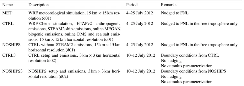
The WRF-Chem simulations performed in this study are summarized in Table 3. The CTRL simulation uses the set-tings and emissions presented above, as well as ship emis-sions produced by the model STEAM2 (Sect. 3.3). The NO-SHIPS simulation is similar to CTRL, but does not include ship emissions. The NOSHIPS and CTRL simulations are carried out from 4 to 25 July 2012, over the 15 km × 15 km simulation domain presented in Fig. 1a. The CTRL3 and NO-SHIPS3 simulations are similar to CTRL and NOSHIPS, but are run on a smaller 3 km × 3 km resolution domain, shown in Fig. 1b, from 10 to 13 July 2012. The CTRL3 and NO-SHIPS3 simulations are not nudged to FNL and do not in-clude a subgrid parameterization for cumulus due to their high resolution. Boundary conditions for CTRL3 and NO-SHIPS3 are taken from the CTRL and NOSHIPS simulations (using one-way nesting within WRF-Chem) and are updated every hour.
The CTRL and CTRL3 simulations are not nudged to the reanalysis fields in the boundary layer, in order to ob-tain a more realistic boundary layer structure. However, comparison with ACCESS meteorological measurements
Table 3. Description of WRF and WRF-Chem simulations.
Name Description Period Remarks
MET WRF meteorological simulation, 15 km × 15 km res-olution (d01)
4–25 July 2012 Nudged to FNL CTRL WRF-Chem simulation, HTAPv2 anthropogenic
emissions, STEAM2 ship emissions, online MEGAN biogenic emissions, online DMS and sea salt emis-sions, 15 km × 15 km horizontal resolution (d01)
4–25 July 2012 Nudged to FNL in the free troposphere only
NOSHIPS CTRL without STEAM2 emissions, 15 km × 15 km horizontal resolution (d01)
4–25 July 2012 Nudged to FNL in the free troposphere only CTRL3 CTRL setup and emissions, 3 km × 3 km horizontal
resolution (d02)
10–12 July 2012 Boundary conditions from CTRL No nudging
No cumulus parameterization NOSHIPS3 NOSHIPS setup and emissions, 3 km × 3 km
hori-zontal resolution (d02)
10–12 July 2012 Boundary conditions from NOSHIPS No nudging
No cumulus parameterization
shows that on 11 July 2012 this leads to an overestimation of marine boundary layer wind speeds (normalized mean bias = +38 %). Since wind speed is one of the most critical parameters in the FLEXPART-WRF simulations, we decided to drive FLEXPART-WRF with the MET simulation instead of using CTRL or CTRL3. In the MET simulation, results are also nudged to FNL in the boundary layer in order to reproduce wind speeds (normalized mean bias of +14 % on 11 July 2012). All CTRL, NOSHIPS, CTRL3, NOSHIPS3 and MET simulations agree well with meteorological mea-surements during the other ACCESS ship flights.
3.3 High-resolution ship emissions from STEAM2
STEAM2 is a high-resolution, real-time bottom-up shipping emissions model based on AIS positioning data (Jalkanen et al., 2012). STEAM2 calculates fuel consumption for each ship based on its speed, engine type, fuel type, vessel length, and propeller type. The model can also take into account the effect of waves, and distinguishes ships at berth, maneuver-ing ships, and cruismaneuver-ing ships. Contributions from weather ef-fects were not included in this study, however. The presence of AIS transmitters is mandatory for large ships (gross ton-nage > 300 t) and voluntary for smaller ships.
Emissions from STEAM2 are compared with emissions derived from measurements for individual ships in Sect. 4. STEAM2 emissions of CO, NOx, OC, BC (technically
ele-mental carbon in STEAM2), sulfur oxides (SOx), SO4, and
exhaust ashes are also used in the WRF-Chem CTRL and CTRL3 simulations. SOxare emitted as SO2in WRF-Chem,
and NOxare emitted as 94 % NO, and 6 % NO2(EPA, 2000).
VOC emissions are estimated from STEAM2 CO emissions using a bulk VOC / CO mass ratio of 53.15 %, the ratio used in the Arctic ship inventory from Corbett et al. (2010). STEAM2 emissions were generated on a 5 km × 5 km grid every 30 min for the CTRL simulation, and on a 1 km × 1 km
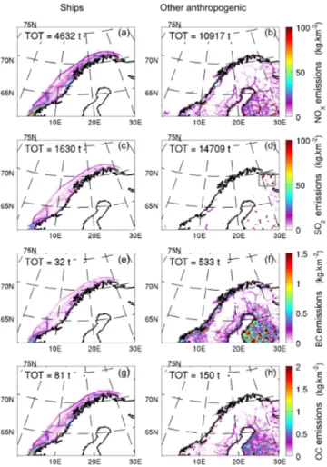
grid every 15 min for the CTRL3 simulation, and were re-gridded on the WRF-Chem simulation grids. Shipping emis-sions of NOx, SO2, black carbon, and organic carbon are
presented in Fig. 2 for the 15 km × 15 km simulation do-main (emissions totals during the simulation period are indi-cated within the figure panels). For comparison, the HTAPv2 emissions (without shipping emissions) are also shown. Ship emissions are, on average, located in main shipping lanes along the Norwegian coastline. However, they also include less traveled routes, which are apparent closer to shore. Other anthropogenic emissions are mainly located along the Nor-wegian coast (mostly in southern Norway) or farther inland and to the south in Sweden and Finland. Over the whole domain, NOxand OC emissions from shipping are
approxi-mately one-third of total anthropogenic NOx and OC
emis-sions, but represent a lower proportion of anthropogenic SO2
and BC emissions (5 and 10 %, respectively). However, other anthropogenic emissions are not co-located with shipping emissions, which represent an important source further north along the coast, as many ships are in transit between Euro-pean ports and Murmansk in Russia. Very strong SO2
emis-sions in Russia are included in the model domain (in the area highlighted in Fig. 2d), associated with smelting activities that occur on the Russian Kola Peninsula (Virkkula et al., 1997; Prank et al., 2010). The Kola Peninsula emissions rep-resent 79 % of the total HTAPv2 SO2 emissions in the
do-main.
STEAM2 emissions are based on AIS signals that are transmitted to base stations on shore that have a limited range of 50–90 km, which explains why the emissions pre-sented in Fig. 2 only represent near-shore traffic. In addi-tion, our study is focused on shipping emissions in north-ern Norway, therefore STEAM2 emissions were only gener-ated along the Norwegian coast. As a result, ship emissions in the northern Baltic and along the northwestern Russian coast are not included in this study. However, these missing
Figure 2. (a, c, e, g) STEAM2 ship emissions and (b, d, f, h) HTAPv2 anthropogenic emissions (without ships) of (a, b) NOx,
(c, d) SO2, (e, f) BC, and (g, h) OC in kg km−2over the CTRL
and NOSHIPS WRF-Chem domain, during the simulation period (00:00 UTC 4 July 2012 to 00:00 UTC 26 July 2012). On panel (d), the location of the intense Kola Peninsula SO2emissions is
high-lighted by a gray box. The emissions totals for the simulation period are noted in each panel.
shipping emissions are much lower than other anthropogenic sources inside the model domain. In the CTRL and CTRL3 simulations, ship emissions are injected in altitude using the plume rise model presented in Sect. 3.1. Stack height and exhaust fluxes are unknown for most of the ships present in the STEAM2 emissions, which were not specifically targeted during ACCESS. For these ships, exhaust parameters for the
Wilson Leer (∼ 6000 gross tonnage) are used as a
compro-mise between the smaller fishing ships (∼ 40 % of Arctic shipping emissions; Winther et al., 2014), and larger ships like the ones targeted during ACCESS. In the CTRL3 sim-ulation, the four ships targeted during ACCESS are usually alone in a 3 km × 3 km grid cell, which enabled us to treat these ships separately and to inject their emissions in alti-tude using individual exhaust parameters (Sect. 3.1). In the CTRL simulation, there are usually several ships in the same 15 km × 15 km grid cell, and the four targeted ships were
treated in the same way together with all unidentified ships, using the exhaust parameters of the Wilson Leer and local meteorological conditions to estimate injection heights. This means that, for the Costa Deliziosa, Alaed and Wilson
Nan-jing, the plume rise model is used in CTRL with exhaust
parameters from a smaller ship (the Wilson Leer) than in CTRL3. Because of this, emission injection heights for these ships are lower in CTRL (0 to 30 m) than in CTRL3 (230 m for the Costa Deliziosa, 50 m for the Wilson Nanjing, 30 m for the Wilson Leer, and 65 m for the Alaed).
Primary aerosol emissions from STEAM2 (BC, OC, SO4,
and ash) are distributed into the eight MOSAIC aerosol bins in WRF-Chem, according to the mass size distribution mea-sured in the exhaust of ships equipped with medium-speed diesel engines by Lyyranen et al. (1999). The submicron mode of this measured distribution is used to distribute pri-mary BC, OC, and SO=4, while the coarse mode is used to distribute exhaust ash particles (represented as “other inor-ganics” in MOSAIC).
4 Ship emission evaluation
In this section, emissions of NOxand SO2are determined for
the four ships sampled during ACCESS flights (shown in Ta-ble 1). We compare airborne measurements in ship plumes and concentrations predicted by FLEXPART-WRF plume dispersion simulations. In order to derive emission fluxes, good agreement between measured and modeled plume lo-cations is required (discussed in Sect. 4.1). The methods, derived emissions values for the four ships, and comparison with STEAM2 emissions are presented in Sect. 4.2.
4.1 Ship plume representation in FLEXPART-WRF and comparison with airborne measurements
FLEXPART-WRF plume dispersion simulations driven by the MET simulation are performed for the four ships sam-pled during ACCESS (Sect. 3.1). The MET simulation agrees well with airborne meteorological measurements on both days (shown in the Supplement, Fig. S1) in terms of wind direction (mean bias of −16◦on 11 July, +6◦ on 12 July) and wind speed (normalized mean bias of +14 % on 11 July,
−17 % on 12 July). Figure 3 shows the comparison between maps of the measured NOxand plume locations predicted by
FLEXPART-WRF. This figure also shows the typical mean-dering pattern of the plane during ACCESS, measuring the same ship plumes several times as they age, while moving further away from the ship (Roiger et al., 2015). Wilson Leer and Costa Deliziosa plumes were sampled during two dif-ferent runs at two altitudes on 11 July 2012, and presented in Fig. 3a and b (z = 49 m) and Fig. 3c and d (z = 165 m). During the second altitude level on 11 July (Fig. 3c and d) the Wilson Leer was farther south and the Costa Deliziosa had moved further north. Therefore, the plumes are farther
Figure 3. Left panels: ACCESS airborne NOx measurements be-tween (a) 16:00 and 16:35 UTC, 11 July 2012 (flight leg at Z ∼ 49 m), (c) 16:52 and 18:08 UTC, 11 July 2012 (Z ∼ 165 m), and
(e) 10:53 and 11:51 UTC, 12 July 2012 (Z ∼ 46 m). Right panels:
corresponding FLEXPART-WRF plumes (relative air tracer mix-ing ratios): (b, d) Wilson Leer and Costa Deliziosa plumes and
(f) Wilson Nanjing and Alaed plumes. FLEXPART-WRF plumes are
shown for the closest model time step and vertical level.
apart than during the first pass at 49 m. Modeled and mea-sured plume locations agree well for the first run (z = 49 m). For the second run (z = 165 m), the modeled plume for the
Costa Deliziosa is, on average, located 4.7 km to the west of
the measured plume. This displacement is small considering that, at the end of this flight leg, the plume was being sampled
∼80 km away from its source. This displacement is caused by biases in the simulation (MET) used to drive the plume dispersion model (−16◦for wind direction, +14 % for wind
speed). On 12 July 2012, the aircraft targeted emissions from the Wilson Nanjing ship (Fig. 3e and f), but also sampled the plume of another ship, the Alaed. This last ship was identified during the post-campaign analysis, and we were able to ex-tract its location and emissions from the STEAM2 inventory in order to perform the plume dispersion simulations shown here. The NOxand FLEXPART-WRF predicted plume
loca-tions are in good agreement for both ships.
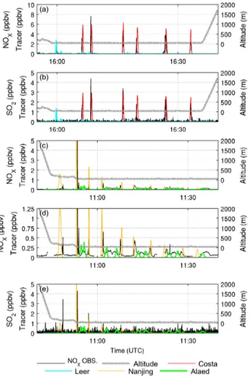
Modeled air tracer mixing ratios are interpolated in space and time to the aircraft location, and compared with airborne NOx and SO2 measurements (Fig. 4). Each peak in Fig. 4
corresponds to the aircraft crossing the ship plume once dur-ing the meanderdur-ing pattern before turndur-ing around for an ad-ditional plume crossing. Figure 4a and b only show measure-ments for the first altitude level at z = 49 m on 11 July 2012 (results for the second altitude level are shown in the Supple-ment in Fig. S2). As expected from the comparison shown in Fig. 3, modeled peaks are co-located with measured peaks in Fig. 4. The model is also able to reproduce the gradual de-crease of concentrations measured in the plume of the Wilson
Nanjing on Fig. 4c–e, as the plane flies further away from the
ship and the plume gets more dispersed. These peak concen-trations vary less for the measured and modeled plume of the
Costa Deliziosa (Fig. 4a and b). Measured plumes are less
concentrated for the Wilson Leer since it is a smaller vessel, and for the Alaed because its emissions were sampled further away from their source.
4.2 Ship emission derivation and comparison with STEAM2
In this section, we describe the method for deriving ship emissions of NOx and SO2 using FLEXPART-WRF and
measurements. This method relies on the fact that in the FLEXPART-WRF simulations presented in Sect. 3.1, there is a linear relationship between the constant emission flux of the tracer chosen for the simulation and the tracer concentra-tions in the modeled plume. The only source of non-linearity that cannot be taken into account is changes in the emission source strength, which is assumed to be constant in time for the plumes sampled. Given that the ship and meteorologi-cal conditions were consistent during sampling (shown in the Supplement, Fig. S1), we expect that these effects would be very small. In our simulations, this constant emission flux is picked at E = 0.1 kg s−1and is identical for all ships. This initial value E is scaled for each ship by the ratio of the mea-sured and modeled areas of the peaks in concentration corre-sponding to plume crossings, as shown in Fig. 4. Equation (1) shows how SO2emissions are derived by this method.
Ei =E × Rtiend tibegin(SO2(t ) −SO2background) dt Rtiend tibeginTracer(t)dt ×MSO2 Mair (1)
In Eq. (1), SO2(t )is the measured SO2mixing ratio (pptv),
SO2background is the background SO2mixing ratio for each
peak, Tracer(t) is the modeled tracer mixing ratio interpo-lated along the ACCESS flight track (pptv), tibeginand tiendare the beginning and end time of peak i (modeled or measured, in s) and MSO2 and Mair are the molar masses of SO2 and
air (g mol−1). This method produces a different SO2
emis-sion flux value Ei (kg s−1) for each of the i = 1 to N peaks
Figure 4. (a, c, d) NOx and (b, e) SO2 aircraft measurements
(black) compared to FLEXPART-WRF air tracer mixing ratios in-terpolated along flight tracks, for the plumes of the (a, b) Costa
Deliziosa and Wilson Leer on 11 July 2012 (first constant altitude
level (Z ∼ 49 m), also shown in Fig. 3a) and (c, d, e) Wilson
Nan-jing and Alaed on 12 July 2012. Panel (d) shows the same results
as panel (c) in detail. Since model results depend linearly on the emission flux chosen a priori for each ship, model results have been scaled so that peak heights are comparable to the measurements.
by the aircraft. These N different estimates are averaged to-gether to reduce the uncertainty in the estimated SO2
emis-sions. A similar approach is used to estimate NOxemissions.
The background mixing ratios were determined by applying a 30 s running average to the SO2 and NOx measurements.
Background values were then determined manually from the filtered time series. For each NOx peak, an individual
back-ground value was identified and used to determine the NOx
enhancement for the same plume. For SO2, a single
back-ground value was used for each flight leg (constant altitude). In order to reduce sensitivity to the calculated emission injection heights, FLEXPART-WRF peaks that are sensitive to a ±50 % change in injection height are excluded from the analysis. Results are considered sensitive to injection
heights if the peak area in tracer concentration changes by more than 50 % in the injection height sensitivity runs. Us-ing a lower threshold of 25 % alters the final emission es-timates by less than 6 %. Peaks sensitive to the calculated injection height typically correspond to samplings close to the ship, where the plumes are narrow. An intense SO2peak
most likely associated with the Costa Deliziosa and sampled around 17:25 UTC on 11 July 2012 is also excluded from the calculations, because this large increase in SO2in an older,
diluted part of the ship plume suggests contamination from another source. SO2 emissions are not determined for the Wilson Leer and the Alaed, since SO2measurements in their
plumes are too low to be distinguished from the background variability. For the same reason, only the higher SO2peaks
(four peaks > 1 ppbv) were used to derive emissions for the
Wilson Nanjing. The number of peaks used to derive
emis-sions for each ship is N = 13 for the Costa Deliziosa, N = 4 for the Wilson Leer, N = 8 for the Wilson Nanjing (N = 4 for SO2) and N = 5 for the Alaed.
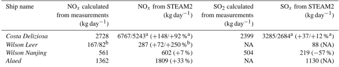
The derived emissions of NOx(equivalent NO2mass flux
in kg day−1) and SO2 are given in Table 4. The emissions
extracted from the STEAM2 inventory for the same ships during the same time period are also shown. STEAM2 SO2
emissions are higher than the value derived for the Costa
Deliziosa, and lower than the value derived for the Wilson Nanjing. NOxemissions from STEAM2 are higher than our
calculations for all ships. In STEAM2, the NOxemission
fac-tor is assigned according to IMO MARPOL (marine pollu-tion) Annex VI requirements (IMO, 2008) and engine revolu-tions per minute (RPM), but all engines subject to these lim-its must emit less NOx than this required value. For the
Wil-son Leer, two calculated values are reported: one calculated
by averaging the estimates from the four measured peaks, and one value where an outlier value was removed before calculating the average. During the 11 July flight, the Wilson
Leer was traveling south at an average speed of 4.5 m s−1, with relatively slow tailwinds of 5.5 m s−1. Because of this, the dispersion of this ship’s plume on this day could be sensi-tive to small changes in modeled wind speeds, and calculated emissions are more uncertain.
The most important difference between the inventory NOx
and our estimates is ∼ 150 % for the Costa Deliziosa. Rea-sons for large discrepancy in predicted and measured NOx
emissions of Costa Deliziosa were investigated in more de-tail. A complete technical description of Costa Deliziosa was not available, but her sister vessel Costa Luminosa was described at length recently (RINA, 2010). The details of
Costa Luminosa and Costa Deliziosa are practically
identi-cal and allow for in-depth analysis of emission modeling. With complete technical data, the STEAM2 SOx and NOx
emissions of Costa Deliziosa were estimated to be 2684 and 5243 kg day−1, respectively, whereas our derived estimates indicate 2399 and 2728 kg day−1 (difference of +12 % for SOxand +92 % for NOx). The good agreement for SOx
Table 4. NOx and SO2emissions estimated from FLEXPART-WRF and ACCESS measurements, compared with STEAM2 emissions.
Values in parentheses indicate the relative difference between STEAM2 and calculated values. SO2emissions were not calculated for the
Wilson Leer and Alaed since the measured SO2concentrations in the plumes were too low above background.
Ship name NOxcalculated NOxfrom STEAM2 SO2calculated SOxfrom STEAM2 from measurements (kg day−1) from measurements (kg day−1)
(kg day−1) (kg day−1)
Costa Deliziosa 2728 6767/5243a(+148/+92 %a) 2399 3285/2684a(+37/+12 %a)
Wilson Leer 167/82b 287 (+72/+250 %b) NA 88 (NA)
Wilson Nanjing 561 602 (+7 %) 504 219 (−57 %)
Alaed 1362 1809 (+33 %) NA 1130 (NA)
aThe second value corresponds to STEAM2 calculations using complete technical data from the Costa Deliziosa sister ship Costa Luminosa.bValue with outliers
removed.
AIS and associated fuel flow is well predicted by STEAM2, but emissions of NOxare twice as high as the value derived
from measurements. In case of Costa Deliziosa, the NOx
emission factor of 10.5 g kWh−1for a tier II compliant ves-sel with 500 RPM engine is assumed by STEAM2. Based on the measurement-derived value, a NOxemission factor of
5.5 g kWh−1would be necessary, which is well below the tier II requirements. It was reported recently (IPCO, 2015) that NOx emission reduction technology was installed on Costa
Deliziosa, but it is unclear whether this technology was in
place during the airborne measurement campaign in 2012. The case of Costa Deliziosa underlines the need for accu-rate and up-to-date technical data for ships when bottom-up emission inventories are constructed. It also necessitates the inclusion of the effect of emission abatement technologies in ship emission inventories. Furthermore, model predictions for individual vessels are complicated by external contribu-tions, like weather and sea currents, affecting vessel perfor-mance. However, the STEAM2 emission model is based on AIS real-time positioning data, which has a much better cov-erage than activity data sets used to generate older shipping emission inventories (e.g., COADS and AMVER). These earlier data sets also have known biases for ships of specific sizes or types. In addition, components of the STEAM2 in-ventory, such as fuel consumption, engine loads, and emis-sion factors have already been studied in detail in the Baltic Sea by Jalkanen et al. (2009, 2012) and Beecken et al. (2015). Beecken et al. (2015) compared STEAM2 emission factors to measurements for ∼ 300 ships in the Baltic Sea. Their re-sults showed that, while important biases were possible for individual ships, STEAM2 performed much better on aver-age for a large fleet. In the Baltic Sea, STEAM2 NOx
emis-sion factors were found to be biased by +4 % for passen-ger ships, based on 29 ships, and −11 % for cargo ships, based on 118 ships. For SOx, the biases were respectively +1
and +14 % for the same ships. Therefore, we expect that the large discrepancy in NOxfor one individual ship (the Costa
Deliziosa) has only a small impact on the total regional
emis-sions generated by STEAM2. The results presented later in Sect. 5.1 also indicate that STEAM2 likely performs better
on average in the Norwegian Sea during ACCESS than for individual ships.
4.3 Comparison of STEAM2 to other shipping emission inventories for northern Norway
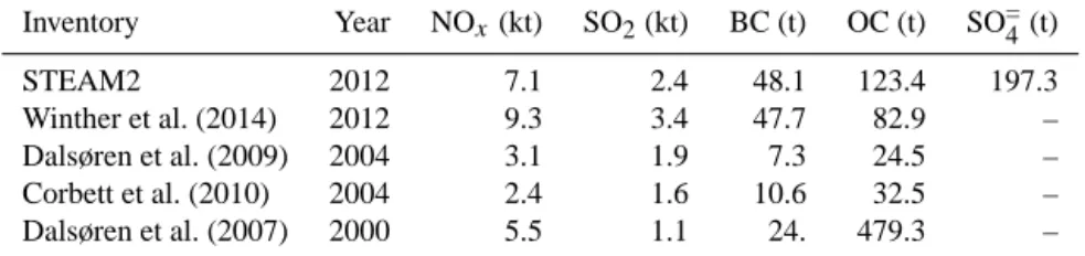
We compare in Table 5 the July emission totals for NOx,
SO2, BC, OC and SO=4 in northern Norway (latitudes 60.6
to 73◦N, longitudes 0 to 31◦W) for STEAM2 and four other shipping emission inventories used in previous studies inves-tigating shipping impacts in the Arctic. We include emissions from the Winther et al. (2014), Dalsøren et al. (2009, 2007), and Corbett et al. (2010) inventories. The highest shipping emissions in the region of northern Norway are found in the STEAM2 and Winther et al. (2014) inventories, which are both based on 2012 AIS ship activity data (Sect. 3.3 for a de-scription of the methodology used for STEAM2). We note that, except for OC, the emissions are higher in the Winther et al. (2014) inventory because of the larger geographical coverage: Winther et al. (2014) used both ground-based and satellite retrieved AIS signals, whereas the current study is restricted to data received by ground based AIS stations (cap-turing ships within 50 to 90 km of the Norwegian coastline). Despite lower coverage, the horizontal and temporal resolu-tions are better described in land-based AIS networks than satellite AIS data. The terrestrial AIS data used in this study is thus more comparable to the spatial extent and temporal resolution of the measurements collected close to the Nor-wegian coast. STEAM2 is the only inventory including sul-fate emissions, which account for SO2to SO=4 conversion in
the ship exhaust. Ship emissions from Dalsøren et al. (2009) and Corbett et al. (2010) are based on ship activity data from 2004, when marine traffic was lower than in 2012. Further-more, the gridded inventory from Corbett et al. (2010) does not include emissions from fishing ships, which represent close to 40 % of Arctic shipping emissions (Winther et al., 2014). These emissions could not be precisely distributed geospatially using earlier methodologies, since fishing ships do not typically follow a simple course (Corbett et al., 2010). Dalsøren et al. (2007) emissions for coastal shipping in
Nor-Table 5. July emission totals in northern Norway (60.6–73◦N, 0 to 31◦W) of NOx, SO2, BC, OC, and SO=4 in different ship emission inventories. Inventory Year NOx(kt) SO2(kt) BC (t) OC (t) SO=4(t) STEAM2 2012 7.1 2.4 48.1 123.4 197.3 Winther et al. (2014) 2012 9.3 3.4 47.7 82.9 – Dalsøren et al. (2009) 2004 3.1 1.9 7.3 24.5 – Corbett et al. (2010) 2004 2.4 1.6 10.6 32.5 – Dalsøren et al. (2007) 2000 5.5 1.1 24. 479.3 –
wegian waters are estimated based on Norwegian shipping statistics for the year 2000, and contain higher NOx, BC,
and OC emissions, but less SO2, than the 2004 inventories.
This comparison indicates that earlier ship emission inven-tories usually contain lower emissions in this region, which can be explained by the current growth in shipping traffic in northern Norway. This means that up-to-date emissions are required in order to assess the current impacts of shipping in this region.
5 Modeling the impacts of ship emissions along the Norwegian coast
In this section, WRF-Chem, using STEAM2 ship emissions, is employed to study the influence of ship pollution on at-mospheric composition along the Norwegian coast, at both the local (i.e., at the plume scale) and regional scale. As shown in Fig. 4, shipping pollution measured during AC-CESS is inhomogeneous, with sharp NOxand SO2peaks in
thin ship plumes, emitted into relatively clean background concentrations. The measured concentrations are on spa-tial scales that can only be reproduced using very high-resolution WRF-Chem simulations (a few kilometers of hor-izontal resolution), but such simulations can only be per-formed for short periods and over small domains. Therefore, high-resolution simulations cannot be used to estimate the regional impacts of shipping emissions. In order to bridge the scale between measurements and model runs that can be used to make conclusions about the regional impacts of ship-ping pollution, we compare in Sect. 5.1 WRF-Chem simu-lations using STEAM2 ship emissions, at 3 km × 3 km res-olution (CTRL3) and at 15 km × 15 km resres-olution (CTRL). Specifically, we show in Sect. 5.1 that both the CTRL3 and CTRL simulations reproduce the average regional influence of ships on NOx, O3, and SO2, compared to ACCESS
mea-surements. In Sect. 5.2 we use the CTRL simulation to quan-tify the regional contribution of ships to surface pollution and shortwave radiative fluxes in northern Norway.
5.1 Model evaluation from the plume scale to the regional scale
It is well known that ship plumes contain fine-scale features that cannot be captured by most regional or global chem-ical transport models. This fine plume structure influences the processing of ship emissions, including O3and aerosol
formation, which are non-linear processes that largely de-pend on the concentration of species inside the plume. Some models take into account the influence of the instantaneous mixing of ship emissions in the model grid box by includ-ing corrections to the O3 production and destruction rates
(Huszar et al., 2010) or take into account plume ageing be-fore dilution by using corrections based on plume chemistry models (Vinken et al., 2011). Here, we take an alternative approach by running the model at a sufficient resolution to distinguish individual ships in the Norwegian Sea (CTRL3 run at 3 km × 3 km resolution), and at a lower resolution (CTRL run at 15 km × 15 km resolution). It is clear that a 3 km × 3 km horizontal resolution is not sufficiently small to capture all small-scale plume processes. However, by com-paring the CTRL3 simulation to ACCESS measurements, we show in this section that this resolution is sufficient to resolve individual ship plumes and to reproduce some of the plume macroscopic properties. The CTRL and CTRL3 simulations (presented in Table 3) are then compared to evaluate if non-linear effects are important for this study period and region.
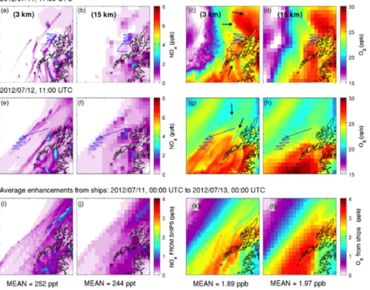
WRF-Chem results from CTRL and CTRL3 for surface (∼ 0 to 30 m) NOx and O3are shown in Fig. 5. On 11 and
12 July, the aircraft specifically targeted plumes from the
Wil-son Leer, Costa Deliziosa, WilWil-son Nanjing and, in addition,
sampled emissions from the Alaed, identified later during the post-campaign analysis (Fig. 3). All these ships are individ-ually present in the STEAM2 emissions inventory (Sect. 4 and Table 4). Emissions from these ships, as well as from other vessels traveling in that area, are clearly resolved in the CTRL3 model results for NOx (Fig. 5a and e). Ship NOx
emissions are smoothed out in the CTRL run, seen in Fig. 5b and f, and the individual ship plumes cannot be clearly dis-tinguished in the NOxsurface concentrations. The predicted
surface O3concentrations are shown in Fig. 5c, d, g, and h.
On the 11 and 12 July 2012, titration of O3 by NOx from
fresh ship emissions can be identified in Fig. 5c and g for the 3 km run (areas indicated by black arrows on Fig. 5c
Figure 5. Snapshots of model predicted surface NOxand O3from the CTRL3 (3 km) simulation (a, c, e, g) and the CTRL (15 km)
simula-tion (b, d, f, h) during the flights on 11 and 12 July 2012. Model results for the CTRL3 simulasimula-tion are shown over the full model domain. CTRL run results are shown over the same region for comparison. The aircraft flight tracks are indicated in blue. On panels (c) and (g), black arrows indicate several areas of O3titration due to high NOxfrom ships. (i, j) NOxand (k, l) O32-day average surface enhancements
(00:00 UTC 11 July 2012 to 00:00 UTC 13 July 2012) due to shipping emissions, (i, k) CTRL3 simulation, (j, l) CTRL simulation. The 2-day average enhancements of NOxand O3over the whole area are given below each respective panel.
and g). However, evidence for O3 titration quickly
disap-pears away from the fresh emissions sources. In contrast, O3titration is not apparent in the CTRL run. However, NOx
and O3patterns and average surface concentrations are very
similar. This is illustrated in the lower panels, showing 2-day-averaged NOxand O3enhancements due to ships in the
CTRL3 (CTRL3 – NOSHIPS3) and CTRL (CTRL – NO-SHIPS) simulations. The results show that changing the hor-izontal resolution from 3 km × 3 km (1 km × 1 km emissions, 15 min emissions injection) to 15 km × 15 km (5 km × 5 km emissions, 1 h emissions injection) does not have a large in-fluence on the domain-wide average NOx (−3.2 %) or O3
(+0.08 ppbv, +4.2 %) enhancements due to ships. This is in agreement with earlier results by Cohan et al. (2006), who showed that regional model simulations at similar resolu-tions (12 km) were sufficient to reproduce the average O3
response. Results by Vinken et al. (2011) suggest that sim-ulations at a lower resolution more typical of global models (2◦×2.5◦) would lead to an overestimation of O3
produc-tion from ships in this region by 1 to 2 ppbv. The influence of model resolution on surface aerosol concentrations is also moderate, and PM10due to ships are 15 % lower on average
in CTRL than in CTRL3 (not shown here).
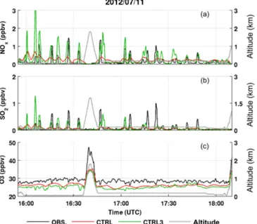
To further investigate the ability of these different model runs to represent single ship plumes, we compare measured NOx, SO2, and O3 along the flight track on 11 July 2012
with WRF-Chem predictions (Fig. 6). Corresponding results for 12 July 2012 are shown in the Supplement (Fig. S3). Large enhancements of NOxand SO2are seen during plume
crossings in measurements, as already noted in Sect. 4. For comparison with WRF-Chem, we have averaged the mea-sured data using a 56 s running average, equivalent to the aircraft crossing 6 km (two model grid cells) at its average speed during this flight (107 m s−1). Using a running
aver-age takes into account plume dilution in grid cells, as well as additional smoothing introduced when modeled results are spatially interpolated onto the flight track. The CTRL3 sim-ulation captures both the width and magnitude of NOx and
SO2 peaks, suggesting that the individual plumes are
cor-rectly represented in space and time. During the second part of the flight (17:20 UTC), the model does not reproduce two intense measured SO2peaks. We already noted in Sect. 4.2
that measurements in this part of the flight might be contami-nated by another source. In contrast, the CTRL run has wider NOxand SO2peaks and lower peak concentrations, because
of dilution in larger grids. Another difference between the simulations is the treatment of plume rise (Sect. 3.3), such
Figure 6. Time series of measured O3and NOxon 11 July 2012 compared to model results extracted along the flight track for the CTRL and CTRL3 runs. Observations are in black, the CTRL run is in red, and the CTRL3 run is in green. A 56 s averaging window is applied to the measured data for model comparison (approximately the time for the aircraft to travel 2 × 3 km). Flight altitude is given as a dashed gray line. After the first run at 49 m, a vertical profile was performed (16:35 to 16:45 UTC) providing information about the vertical structure of the boundary layer.
that the Costa Deliziosa plume is located at lower altitudes in CTRL than in CTRL3. The CTRL3 simulation tends to overestimate NOx in ship plumes, which is in agreement
with the results shown in Table 4, indicating that STEAM2 NOxemissions are overestimated for the ships targeted
dur-ing ACCESS. This overestimation is unlikely to be caused by chemistry issues, since an overestimated NOx lifetime
would lead to comparatively larger biases at the end of the constant altitude runs, when older parts of the plume were sampled. Figure 6b shows O3 during the same flight. The
CTRL3 simulation reproduces the ozone variability better than the CTRL run, but both runs perform relatively well on average (mean bias = −3 ppbv during the constant altitude legs). This negative bias is due to a small underestimation in the background ozone, which could be caused by a num-ber of reasons, including the boundary chemical conditions from the MOZART4 model, photolysis rates, cloud proper-ties and locations, ozone deposition, and/or emissions. Both measurements and CTRL3 results show evidence of O3
titra-tion in the most concentrated NOx plumes, where ozone is
1.5 to 3 ppbv lower than out of the plumes. However, precise quantification of this titration is difficult because these val-ues are the same order of magnitude as the spatial variability of O3outside of the plumes. O3 titration is not apparent in
the CTRL run. Results are similar for the 12 July 2012 flight
Figure 7. Observed background-corrected PM1 enhancements in
the plume of the Costa Deliziosa on 11 July 2012 (black squares), compared to modeled PM1enhancements in ship plumes (in red),
extracted along the flight track (CTRL3 – NOSHIPS3 PM1). A 56 s
averaging window is applied to the measured data to simulate dilu-tion in the model grid. Flight altitude is given as dashed black line.
(shown in the Supplement, Fig. S3), with lower model biases for O3but a stronger overestimation of NOx.
In order to evaluate modeled aerosols in ship plumes, mod-eled aerosols are evaluated using size distributions measured during the 11 July 2012 flight. Size distributions are inte-grated to estimate submicron aerosol mass (PM1), assuming
a density of 1700 kg m−3and spherical particles. This indi-cates that observed PM1enhancements in plumes (∼ 0.1 to
0.5 µg m−3) are relatively low compared to background PM1
(∼ 0.7 to 1.1 µg m−3), because of the presence of high sea salt concentrations in the marine boundary layer (54 % of the modeled background PM1during ship plume sampling is sea
salt in NOSHIPS3). Because of this, comparing modeled and observed in-plume PM1directly would be mostly
represen-tative of background aerosols, especially sea salt, which is not the focus of this paper. Figure 7 shows the comparison between modeled and measured enhancements in PM1in the
plume of the Costa Deliziosa (11 July 2012), removing from the model and measurements the contribution from sea salt and other aerosols not associated with shipping. Similarly to Fig. 6, a 56 s moving average was applied to the measure-ment (representing plume dilution in the model grid). This comparison indicates a generally good agreement between modeled and measured PM1enhancements in ship plumes.
There is a discrepancy between the model and the measure-ments for the first two PM1 plumes measured close to the
ships (around 16:05 UTC), which could be an artifact of the limited resolution of this simulation (3 km). If these peaks are excluded, the model slightly overestimates peak PM1
en-hancements in ship plumes (+26 %). Since this enhancement is modeled as 80 % SO=4, this overestimation can be linked to the +37 % overestimation of SO2 emissions for the Costa Deliziosa in STEAM2 (Table 4).
Analysis of O3maps, average surface enhancements due
to ships (Fig. 5) and analysis of model results along flight tracks (Fig. 6) show that both runs capture the NOx and
Further-Figure 8. Average vertical profiles of (a) NOx, (b) SO2, (c) O3and (d) PM2.5 observed during the four ACCESS ship flights (in black,
with error bars showing standard deviations), and interpolated along the ACCESS flight tracks in the CTRL simulation (red line) and in the NOSHIPS simulation (blue line). For PM2.5only simulation results are shown.
more, Fig. 7 shows that PM1enhancements in ship plumes
are well reproduced in the CTRL3 simulation, and we found that PM10production from ships over the simulation domain
was not very sensitive to resolution. This suggests that the CTRL simulation is sufficient to assess the impacts of ship emissions at a larger scale during July 2012. This is inves-tigated further by comparing modeled NOx, SO2, and O3in
the CTRL and NOSHIPS simulations with the average ver-tical profiles (200–1500 m) measured during four ACCESS flights from 11 to 25 July 2012 (flights shown in Fig. 1a); this comparison is shown in Fig. 8. Modeled vertical profiles of PM2.5are also shown in Fig. 8. This comparison allows us
to estimate how well CTRL represents the average impact of shipping over a larger area and a longer period.
Figure 8 shows that the NOSHIPS simulation significantly underestimates NOx and SO2, and moderately
underesti-mates O3 along the ACCESS flights, indicating that ship
emissions are needed to improve the agreement between the model and observations. In the CTRL simulation, NOx, SO2,
and O3 vertical structure and concentrations are generally
well reproduced, with normalized mean biases of +14.2,
−6.8, and −7.0 %, respectively. Correlations between mod-eled (CTRL) and measured profiles are significant for NOx
and O3(r2=0.82 and 0.90). However, the correlation is very
low between measured and modeled SO2(r2=0.02), and it
is not improved compared to the NOSHIPS simulation. Ships have the largest influence on NOxand SO2profiles, a
moder-ate influence on O3and do not strongly influence PM2.5
pro-files along the ACCESS flights. However, this small increase in PM2.5 corresponds to a larger relative increase in sulfate
concentrations and in particle numbers in the size ranges
typically activated as cloud condensation nuclei (shown in Fig. S4 in the Supplement).
NOx concentrations are overestimated in the parts of the
profile strongly influenced by shipping emissions. This is in agreement with the findings of Sect. 4.2, showing that STEAM2 NOx emissions were overestimated for the ships
sampled during ACCESS. However, the CTRL simulation performs well on average, suggesting that the STEAM2 in-ventory is able to represent the average NOxemissions from
ships along the northern Norwegian coast during the study period. The bias for SO2is very low compared to results from
Eyring et al. (2007), which showed that global models signif-icantly underestimated SO2in the polluted marine boundary
layer in July. Since aerosols from ships contain mostly sec-ondary sulfate formed from SO2oxidation, the validation of
modeled SO2presented in Fig. 8 also gives some confidence
in our aerosol results compared to earlier studies investigat-ing the air quality and radiative impacts of shippinvestigat-ing aerosols. We therefore use the 15 km × 15 km CTRL run for further analysis of the regional influence of ships on pollution and the shortwave radiative effect in this region in Sect. 5.2.
5.2 Regional influence of ship emissions in July 2012 5.2.1 Surface air pollution from ship emissions in
northern Norway
The regional-scale impacts of ships on surface atmospheric composition in northern Norway are estimated by calculat-ing the 15-day (00:00 UTC, 11 July 2012 to 00:00 UTC, 26 July 2012) average difference between the CTRL and NO-SHIPS simulations. Figure 9 shows maps of these
anoma-Figure 9. 15-day average (00:00 UTC 11 July 2012 to 00:00 UTC 26 July 2012) of (top) absolute and (bottom) relative surface enhancements
(CTRL – NOSHIPS) in (a, d) SO2, (b, e) NOx, and (c, e) O3due to ship emissions in northern Norway from STEAM2.
lies at the surface, for SO2, NOx, and O3. Ship emissions
have the largest influence on surface NOx and SO2
concen-trations, with 75 to 100 % increases along the coast. Average O3 increases from shipping are ∼ 6 % (∼ 1.5 ppbv) in the
coastal regions, with slightly lower enhancements (∼ 1 ppbv,
∼4 %,) further inland over Sweden.
Dalsøren et al. (2007) studied the impact of maritime traf-fic in northern Norway in the summer using ship emission estimates for the year 2000. They found, for July 2000, a 1 to 1.5 % increase in surface O3from coastal shipping in
Nor-wegian waters. However, unlike the present study, the esti-mate of Dalsøren et al. (2007) did not include the impact of international transit shipping along the Norwegian coast. Our estimated impact on O3in this region (6 % and 1.5 ppbv
increase) is about half of the one determined by Ødemark et al. (2012) (12 % and 3 ppbv), for the total Arctic fleet in the summer (June–Aug–Sept) 2004, using ship emissions for the year 2004 from Dalsøren et al. (2009). It is important to note that we expect lower impacts of shipping in studies based on earlier years, because of the continued growth of shipping emissions along the Norwegian coast (as discussed in Sect. 4.3 and illustrated in Table 5). However, stronger or lower emissions do not seem to completely explain the differ-ent modeled impacts. Ødemark et al. (2012) found that Arctic ships had a strong influence on surface O3in northern
Nor-way for relatively low 2004 shipping emissions. This could be explained by the different processes included in both mod-els, or by different meteorological situations in the two stud-ies based on two different meteorological years (2004 and 2012). However, it is also likely that the higher O3 in the
Ødemark et al. (2012) study could be caused, in part, by non-linear effects associated with global models run at low
reso-lutions. For example Vinken et al. (2011) estimated that in-stant dilution of shipping NOxemissions in 2◦×2.5◦model
grids leads to a 1 to 2 ppbv overestimation in ozone in the Norwegian and Barents seas during July 2005. This effect could explain a large part of the difference in O3
enhance-ments from shipping between the simulations of Ødemark et al. (2012) (2.8◦×2.8◦resolution) and the simulations pre-sented in this paper (15 km × 15 km resolution).
The impact of ships in northern Norway on surface PM2.5,
BC, and SO=4during the same period is shown in Fig. 10. The impact on PM2.5 is relatively modest, less than 0.5 µg m−3.
However, these values correspond to an important relative increase of ∼ 10 % over inland Norway and Sweden because of the low background PM2.5in this region. Over the sea
sur-face, the relative effect of ship emissions is quite low because of higher sea salt aerosol background. Aliabadi et al. (2014) have observed similar increases in PM2.5(0.5 to 1.9 µg m−3)
in air masses influenced by shipping pollution in the remote Canadian Arctic. In spite of the higher traffic in northern Norway, we find lower values than Aliabadi et al. (2014) be-cause results in Fig. 10 are smoothed by the 15-day average. Impacts on surface sulfate and BC concentrations are quite large, reaching up to 20 and 50 %, respectively. We note that Eckhardt et al. (2013) found enhancements in summertime equivalent BC of 11 % in Svalbard from cruise ships alone. As expected, absolute SO=4and BC enhancements in our sim-ulations are higher in the southern part of the domain, where ship emissions are the strongest. We estimated the lifetime (residence time) of BC originating from ship emissions us-ing the method presented in Samset et al. (2014). This resi-dence time is defined as the ratio of the average BC burden from ships divided by the average BC emissions in STEAM2