System identification of inventory system using ARX and ARMAX models

System Identification of Inventory System Using ARX and

ARMAX Models

Sofia Rachad, Benayad Nsiri and

Bahloul Bensassi

PMMAT laboratory, faculty of sciences Ain Chock Hassan II University,

Casablanca Morocco

LIAD laboratory, faculty of sciences Ain Chock Hassan II University, Casablanca

Morocco

Sofia.rachad@gmail.com,

benayad.nsiri@telecom-bretagne.eu,

c

bensassi@fsac.ac.ma

Abstract

This paper presents a mathematical model of an inventory system from the warehouse of goods Distribution Company using system identification approach. Considering items ordered from suppliers and items shipped to customers, as the inputs of the system and the stock level as the output system. In this paper, ARX model and ARMAX model are outlined and compared. The performances of each type of model are highlighted. A case study with real data set is discussed.

Keywords: System identification, inventory system, Stock level, ARX model, ARMAX

model

1. Introduction

Complex, costly and vulnerable, these are the words that best describe supply chain today, since it faces considerable pressure due to conformity of requirements, suppliers and multiple information flows. Consequently, it is increasingly difficult to meet these challenges.

Although, considerable efforts have been made, using modeling and simulation tools for solving supply chain related problems; their use remains irregular from one environment to another.

The central core of any industrial activity is the triple functions of production, inventory and distribution. In order to meet demand on time, companies must maintain on hand a stock of goods waiting to be sold. Formulating a suitable inventory model is one of the major concerns for an industry. The inventory is studied to help companies reduce costs and regulate stock levels.

In literature, various models have been proposed for inventory systems. To place all the published inventory models in this paper is almost impossible. Sumer c. Aggarwal discussed in [1], the inventory related models from the systems point of view; where he grouped the models in 6 categories: (1) models for determining optimum inventory policies, (2) lot size optimization, (3) optimization of various specific management objectives, (4) models for optimizing highly specialized inventory situations, (5) application of advanced mathematical theories to inventory problems, and (6) models bridging the gap between theory and practice.

Serhii Ziukov explains in [2] that models are classified according to the nature of available information on the system properties: Any model that has parameters well-defined is called a deterministic model. If the parameters of the system are random values, the system is stochastic. He presented also a classification of the models according to their change over time: static models and dynamic models. Inventory systems can also be

classified according to the way the inventory is reviewed, either continuously or periodic as reported in [3] by Jaime Zappone.

Inventory systems are complex due to presence of several types of parameters. In order to optimize and regulate the flow of such systems, we still believe that there is a need of a «"lean » model that describes its dynamic behavior, and to estimate the parameters instead of taking it to pieces and analyzing its parts. And this is exactly one of the basic concepts of system identification.

The identification approach deals with problem of building mathematical model of dynamical systems based on observed data from the system. [5]

The identification system is a fairly mature field that has seen an interesting development and various contributions over the years, that we could not all include in this work, but just a few references that dealt with a parametric models which are ARX, ARMAX, OE and BJ. [9-12]

Many works has been accomplished at this level, however, there's a number of issues in industry, which have not been satisfactorily dealt [4]. In previous study, we proposed “black box" modeling of a production line with three machines from the observed inputs and outputs, using ARX and ARMAX models. [12]

In this paper, we study the case of an inventory system from a distribution company. The inventory system is considered as a MISO system with two input variables and one output variable. The same modeling method in [12], is used to identify the internal properties of the studied system.

The mathematical model of the inventory system, obtained through the identification approach, will allow us to predict inventory changes, variation in demand and lead time. It will also enable to propose suitable control strategies in order to regulate the stock level, so that it could be no stock shortage or overstocking. More details about the system studied are discussed in the following.

The paper is organized as follows. The system identification is introduced in Section II. The inventory system characteristics are described in Section III. In Section IV, some results of the comparative study between ARX and ARMAX are discussed. The paper will be completed by a conclusion and some perspectives.

2. Description of the Studied System

The study was focused on a stock of goods in a distribution company. The warehouse system is characterized by a large number of items and large quantities of goods that it’s kept on stock, in order to satisfy customer demand, which is considered to be stochastic.

The stock is periodically reviewed, and irregularly supplied depending on available stock and variable customer demand. This also known in the literature by fixed procurement lead time and variable quantity order. [8]

The warehouse is managed following a procurement policy, which is a shade of replenishment model. The difference lies in the order up-to level parameter, which is used to determine the size of the order without exceeding a stock max. The order up-to level has not been considered in our case.

The main objective of stock management is to minimize the inventory cost and to define the optimal inventory levels that must be maintained to meet expected service levels for customer demand fulfillment.

In this work, we plan to study the stock as a MISO system through its inputs outputs data. Stock level represents the output variables. Stock level depends on two inputs variables of the system, which are respectively, the quantity ordered from suppliers and the quantity shipped to the customer.

As shown in the Figure 1, u1 and u2 are respectively, the input variables and y is the output variable to be estimated.

Figure1. Multi Input Single Output Inventory System u1: The quantity ordered from suppliers.

u2: The quantity shipped to the customer y: The stock level

e: Disturbances that affect the stock

The inventory items are categorized according to their turnover frequency, which means the ability of a stock to be renewed during a time period [7]. In this paper, we worked on a sample of each category: high turnover items, medium turnover and low turnover.

3. Modeling Method

The modeling method used in this work is the system identification. It is the process that covers the problem of building models of a dynamic system from observed input output signals [5]. The procedure to model a dynamical system based on identification approach is shown in Figure 2.

Figure 2. System Identification Loop [6]

It’s always useful to remind the procedure of identification approach. The construction of the model from extracted data involves four basic steps [5]:

1.1. The acquisition of Dataset

1.2. A set of candidate models and determining the best model in the set 1.3. Parameter estimation 1.4. Validation model Cho o se cr it er io n Co llect da ta M o del set

Estimate model parameters

Validate model Application of selected model ok Not ok Inventory System u1 u2 y e

3.1. The Acquisition of Data Set

Data set is an important part of the identification approach: The acquisition of dataset is the step where we determine which signals to measure and when to measure them. The objective of the experiment design is to make these choices.

In this study case, the data were recorded and collected from a stock system over a time interval.

The set of input output was divided into two parts. The first part was chosen for the estimation step while the second one was chosen for the validation step.

3.2. A Set of Candidate Models and Determining the Best Model in the Set

At this stage, choosing a suitable model structure is prerequisite before to estimate its inner parameters.

The black-box model assumes that the studied system is unknown and all model parameters are adjustable without considering the physical background. In this work, we will focus on linear parametric models. A parametric model structure is also known as a black-box model, which defines either a continuous-time system or a discrete-time system. The principle of system identification based on parametric models is to extract a mathematical model guided by real data.

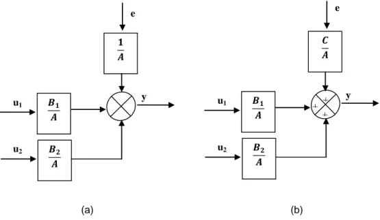
There are few structures of the model that can be used to represent certain systems. In this study, we will consider two simple linear models with multi input single output (MISO). Figure 3 represent those models respectively termed ARX model (Autoregressive with external input) and ARMAX (autoregressive moving average with external input).

Firstly, the ARX model structure is one of the simplest parametric structures. The structure of the ARX model can be written in the form of the equation (1) and the general structure of MISO ARX model is shown in equation (2).

𝐴(𝑞−1_{)𝑦(𝑘 − 𝑛) = 𝑞}−𝑑_𝐵(𝑞−1_{)𝑢(𝑘 − 𝑛) + 𝑒(𝑘) (1)}

𝐴(𝑞−1_{)𝑦(𝑘 − 𝑛) = 𝑞}−𝑑_𝐵

1(𝑞−1)𝑢1(k − n) + 𝑞−𝑑𝐵2(𝑞−1)𝑢2(k − n) + 𝑒(𝑘) (2) The ARMAX model structure is similar to ARX structure, but with an additional term, which represents the moving average error. ARMAX models are useful when dominating disturbances that have enter early in the process. The structure of the ARMAX model can be written in the form of the equation (3) and the general structure of MISO ARMAX model is shown in equation:

𝐴(𝑞−1_{)𝑦(𝑘 − 𝑛) = 𝑞}−𝑑_𝐵(𝑞−1_{)𝑢(𝑘 − 𝑛) + 𝐶(𝑞}−1_{)𝑒(𝑘) (3)}

𝐴(𝑞)𝑦(𝑘 − 𝑛) = 𝑞−𝑑_𝐵

1(q)𝑢1(𝑘 − 𝑛) + 𝑞−𝑑𝐵2(q)𝑢2(𝑘 − 𝑛) + C(q)𝑒(𝑘) (4) Whether it’s the ARX or ARMAX model A(𝑞−1_{), B(𝑞}−1_{) and C(𝑞}−1_{) are} polynomials to be estimated. For the ARX model, the polynomial C(𝑞−1_{) = 1.}

These polynomials represent the overall system dynamics, where A(𝑞−1_{), B(𝑞}−1_{) and} C(𝑞−1_{) are defined by:}

𝐴(𝑞−1_{) = 1 + 𝑎} 1𝑞−1+ ⋯ + 𝑎na𝑞−na (5) 𝐵(𝑞−1_{) = 𝑏} 0+ ⋯ + 𝑏_nb𝑞−𝑛𝑏 𝐶(𝑞−1_{) = 1 + 𝑐} 1𝑞−1+ ⋯ + 𝑐𝑛𝑐𝑞−𝑛𝑐

u(k) and y(k) are respectively the input and the output of the system and e(k) is a white noise signal.. k is time unit and q−1 _{represents the delay operator.}

Variables ai, bj and cl are model parameters to be estimated, with i = 1, … 𝑛𝑎, j =

1, … 𝑛𝑏 l = 1, … 𝑛𝑐. 𝑛 is the pure delay model. The minimum value of 𝑛 is supposed to be equal to 0.

(a) (b)

Figure 3. MISO Linear Parametric Model Structure: (A) MISO ARX Model Structure. (B) MISO ARMAX Model Structure

3.3. Parameter Estimation

Parameter estimation is a process involving mathematical optimization. It comes to choose the accurate method of estimating model parameters or a criterion to be minimized.

In this work, the estimated model is done by using the prediction error method (PEM). The principle of the parameters estimation based on the prediction error method (PEM) is shown in Figure 4.

Figure 4. Parameter Estimation Base on Prediction Error Method

The prediction error is given by:

𝜀(𝑘, 𝜃) = 𝑦(𝑘) − 𝑦̂(𝑘|𝜃) (6)

Where, 𝜀 is the prediction error resulting from y(k) the observed output and ŷ(k|θ) the predicted output. θ is the vector of unknown parameters defined by:

u(t) y(t) Studied system Model Ɛ Criterion 𝑩𝟏 𝑨 𝑩𝟐 𝑨 u1 u2 𝟏 𝑨 e y _𝑩 𝟏 𝑨 𝑩𝟐 𝑨 u1 u2 𝑪 𝑨 y e + + + ŷ(t) +

𝜃𝑇 _{= [𝑎}

1, … , 𝑎𝑛𝑎 𝑏1,, … , 𝑏𝑛𝑏 𝑐1, … , 𝑐𝑛𝑐] (7)

We chose to work with the least squares algorithm (LSA) as a common method used in linear system identification, in order to minimize the prediction error criterion mentioned in (6).The Least squares method is often represented by a function, known also as the loss function. It can be written as:

minθ VN (θ,ZN) (8) Where 𝑉𝑁 (𝜃, 𝑍𝑁) = 1 𝑁∑(𝑦(𝑘) − 𝑦̂(𝑘|𝜃))² 𝑁 𝑘=1 (9)

ZN _{is a set of input outputs data recorded over time interval 1 ≤ 𝑡 ≤ 𝑁 where:} 𝑍𝑁_{= {𝑢(1). 𝑦(1) … 𝑢(𝑁). 𝑦(𝑁)} (10)}

3.4. Model Validation

Model validation is the final step of the system identification process; it involves verifying between the measured data and desired data. Based on this work, we will concentrate the study on few criterions:

3.4.1. Best Fit Criterion:

The best model structure is the one that minimizes the prediction error. Best fit criterion is often used for model validation, by considering the highest fit.

The best fit is measured by the coefficient of determination denoted R2_{, expressed by:}

𝑅2_{= 100 × (1 −} ∑𝑁𝑖=1𝜀2 ∑𝑁 (𝑦 − 𝑦̂ 𝑖=1 )² ) % (11) 3.4.2. FPE Criterion:

The second criterion used in this study is the Final Prediction Error (FPE). It evaluates model quality, where the model is tested on a new set of data. The most accurate model has the smallest FPE.

The FPE equation is defined by the following equation:

𝐹𝑃𝐸 = 𝑉𝑁 (𝜃, 𝑍𝑁) (1 + 𝑑 𝑛

⁄ 1 − 𝑑 𝑛⁄ )

(12)

Where VN (θ, ZN) represent the loss function for the studied structure, d is the total number of estimated data and N is the length of data record.

4. Results and Discussion

The inventory model has been constructed based on measured inputs and outputs data of the system considered as reference.

Inventory items that are the subject of the study have been chosen according to their turnover frequency: High turnover items (HT), medium turnover (MT) and low turnover

0 0.2 0.4 0.6 0.8 1 1.2 1.4 1.6 -1 -0.5 0 0.5 1x 10 4 y 1 :O u tp u t d a ta

Input and output signals

0 0.2 0.4 0.6 0.8 1 1.2 1.4 1.6 -2000 0 2000 4000 Time u 1 : In p u t d a ta

Validation data Estimated data

0 0.2 0.4 0.6 0.8 1 1.2 1.4 1.6 -1 -0.5 0 0.5 1x 10 4 y 1 : O u tp u t d a ta

Input and output signals

0 0.2 0.4 0.6 0.8 1 1.2 1.4 1.6 -100 0 100 200 Time u 2 : In p u t d a ta

Validation data Estimation data

(LT). Data set have been recorded and collected over a time interval between August 2014 and January 2015.

The figure 5 shows measured input output data for each item category. The processing has been carried out by removing means and filtering data. In this paper, the mathematical model of the inventory system is obtained using parametric models such ARX and ARMAX.

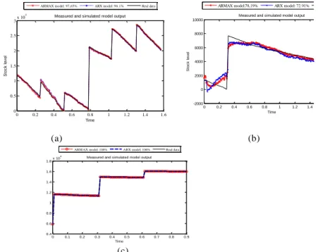
For each category of item, we estimated the output y of system, using the LSA technique. Comparing between ARX and ARMAX model , and varying the number of parameters, we found that the best fit is given by the ARMAX model for the three cases, knowing that it represents, in each case, a lower number of parameters. The figure 6 represents the comparative graph between ARX and ARMAX model for the 3 samples. Besides the best fit, model validation is based also on FPE criterion. Model selection is done according to the smallest FPE. In this study, the ARMAX model gives smallest value of FPE. In the same figure, low turnover items recorded the same best fit for both models, but the smallest FPE was given by the ARMAX model.

The polynomial parameters, as well as all information related to the studied models, are given in Table 1.

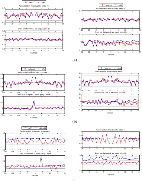
The last step consists in the autocorrelation and cross correlation analyses. Both analyses are considered good when the signal response is within the range set. Figure 7 presents the cross correlation and residual analysis of ARX and ARMAX model for every item sample, and shows that ARMAX fit under the conditions.

(a) (b) 0 0.5 1 1.5 -2 0 2 4x 10 4 y 1 : O u tp u t s ig n a l

Input and output signals

0 0.5 1 1.5 -2 0 2 4x 10 4 Time u 1 : In p u t s ig n a l

Validation data Estimation data

0 0.5 1 1.5 -2 0 2 4x 10 4 y 1 : O u tp u t s ig n a l

Input and output signals

0 0.5 1 1.5 -500 0 500 1000 Time u 2 : in p u t s ig n a l

0 0.1 0.2 0.3 0.4 0.5 0.6 0.7 0.8 0.9 -1 0 1 2x 10 4 y 1 : O u tp u t s ig n a l

Input and output signals

0 0.1 0.2 0.3 0.4 0.5 0.6 0.7 0.8 0.9 0 2000 4000 6000 Time u 1 : In p u t s ig n a l

Validation data Estimation data

0 0.1 0.2 0.3 0.4 0.5 0.6 0.7 0.8 0.9 -1 0 1 2x 10 4 y 1 : O u tp u t

Input and output signals

0 0.1 0.2 0.3 0.4 0.5 0.6 0.7 0.8 0.9 -10 0 10 20 Time u 2 : In p u t 0 0.2 0.4 0.6 0.8 1 1.2 1.4 1.6 0 0.5 1 1.5 2 2.5 3x 10 4 Time S to c k l e v e l

Measured and simulated model output

ARMAX model: 97,65% ARX model: 96.1% Real data

0 0.2 0.4 0.6 0.8 1 1.2 1.4 1.6 1.8 -2000 0 2000 4000 6000 8000 10000 Time S to c k l e v e l

Measured and simulated model output

ARMAX model:78,19% ARX model: 72.91% Real data

(c)

Figure 5. Input Output Signals after Linearization for Each Items Category: (A) Inputs Output Data of High Turnover Items. (B) Inputs Output Data of Medium Turnover Items. (C) Inputs Output Data of Low

Turnover Items

(a) (b)

(c)

Figure 6. Graphic Comparison between Actual Output (Stock Level) and Predicted Output for each Items Category: (A) Graphic Comparison for High Turnover Items (B) Graphic Comparison for Medium Turnover Items (C) Graphic Comparison for Low Turnover

Items 0 0.1 0.2 0.3 0.4 0.5 0.6 0.7 0.8 0.9 0.4 0.6 0.8 1 1.2 1.4 1.6 1.8x 10 4 Time Measured and simulated model output

-20 -15 -10 -5 0 5 10 15 20 -0.2

0 0.2

Autocorrelation of residuals for output y1

-20 -15 -10 -5 0 5 10 15 20 -0.2 -0.1 0 0.1 0.2 Samples Cross corr for input u1 and output y1 resids

ARMAX ARX -20 -15 -10 -5 0 5 10 15 20 -0.5 0 0.5 Autocorrelation of residuals for output y1

-20 -15 -10 -5 0 5 10 15 20 -0.2

0 0.2

Samples Cross corr for input u2 and output y1 resids

ARM AX ARX -20 -15 -10 -5 0 5 10 15 20 -0.2 -0.1 0 0.1 0.2 Autocorrelation of residuals for output y1

-20 -15 -10 -5 0 5 10 15 20 -0.5 0 0.5 1 Samples Cross corr for input u1 and output y1 resids

ARMAX ARX -20 -15 -10 -5 0 5 10 15 20 -0.2 -0.1 0 0.1 0.2 Autocorrelation of residuals for output y1

-20 -15 -10 -5 0 5 10 15 20 -0.2 -0.1 0 0.1 0.2 Samples Cross corr for input u2 and output y1 resids

ARM AX ARX -20 -15 -10 -5 0 5 10 15 20 -0.5 0 0.5 Autocorrelation of residuals for output y1

-20 -15 -10 -5 0 5 10 15 20 -0.5 0 0.5 1 Samples Cross corr for input u1 and output y1 resids

ARX ARMAX -20 -15 -10 -5 0 5 10 15 20 -1 -0.5 0 0.5 1 Autocorrelation of residuals for output y1

-20 -15 -10 -5 0 5 10 15 20 -0.5

0 0.5

Samples Cross corr for input u2 and output y1 resids

(a)

(b)

(c)

Figure 7. Cross Correlation and Residuals Analysis of Arx and Armax Models for each Items Category: (A) Ht (B) Mt (C) Lt

Table 1. Summary of All Models Properties

M odel

Best

Fit R² FPE Linear polynimial Parameters

HT A RX 96.1% 1.273 . 104 A(z) = 1 − 0.9857 z−1 _{− 0.05117z}−2 ₊ 0.07404z−3 _{− 0.03825z}−4 𝐵1(𝑧) =0.9873+0.01416𝑧−1 + 0.03621𝑧−2 + 0.03884𝑧−3 𝐵2(𝑧) =-1.22+0.01416𝑧−1 + 0.02311𝑧−2 − 0.1234𝑧−3 A RMA X 97.65 % 1.225 . 104 𝐴(𝑧) =1-1.909𝑧−1 _{+ 0.9093𝑧}−2 𝐵1(𝑧) =0.9881−0.8974𝑧−1 𝐵2(𝑧) = −1.261 + 1.163𝑧−1 𝐶(𝑧) = 1 − 1.0.13𝑧−1 _{+ 0.01997𝑧}−2

MT A RX 72.91 % 6.368 . 104 𝐴(𝑧) = 1 − 0.9796 𝑧−1 𝐵1(𝑧) =1.034𝑧−1 + 0.02533𝑧−2 + 0.02432𝑧−3 _{− 0.008471𝑧}−4 _{+ 0.06211𝑧}−5 𝐵2(𝑧) =-4.296𝑧−1 + 5.98𝑧−2 − 2.583𝑧−3 − 0.4227𝑧−4 _{+ 4.276𝑧}−5 A RMA X 78.19 % 6.224 . 104 𝐴(𝑧) =1-0.8411𝑧−1 _{− 0.552𝑧}−2 _++0.0559𝑧−3 ₊ 0.3447𝑧−4 𝐵1(𝑧) = 0.9691𝑧−1 + 0.2156𝑧−2 − 0.3392𝑧−3 − 0.4004𝑧−4 𝐵2(𝑧) = −4.086𝑧−1 + 5.995𝑧−2 + 1.613𝑧−3 − 2.39𝑧−4 𝐶(𝑧) = 1+0.2635𝑧−1 _{− 0.5697𝑧}−2 − 0.6784𝑧−3 _{+ 0.004833𝑧}−4 LT A RX 100% 5.153 10−25 𝐴(𝑧) = 1 − 𝑧−1 _{− 6.386 10}−14 _𝑧−3 ₋ 3.574 10−15 _𝑧−4 𝐵1(𝑧) = 3.16 10−17_{+ 𝑧}−1 _{+ 6.712 10}−14 _𝑧−2 ₊ + 6.76 10−14 _𝑧−3 _{− 0.008471 𝑧}−4 𝐵2(𝑧) = −1 − 1.244 10−13𝑧−2 − − 8.288 10−16 _𝑧−3 A RMA X 100% 6.201 10−34 𝐴(𝑧) = 1 – 1 𝑧−1 _{− 4.988 10}−17 _𝑧−2 𝐵1(𝑧) = 1.903 10−19+ 𝑧−1 𝐵2(𝑧) = −1 + 𝑧−1 𝐶(𝑧) = 1 + 0.9654 𝑧−1 _{+ 0.7502 𝑧}−2

5. Conclusion

In this paper, we proposed an inventory model using system

identification, which is consists of building a model from observed data. We

opted for two linear parametric models which are ARX and ARMAX. The

study was conducted on three types of items depending on the turnover

frequency. The comparative study showed that the best linear model is

ARMAX because of its low number of parameters and higher percentage of

best fit, with 97, 65% for the (HT) items and 78.19% for (MT) items and

finally 100% of best fit for the (LT) items. Mathematical inventory model,

will allow us to supervise the system, and thus, to propose appropriate

control strategies.

Acknowledgments

We would like to thanks Mr. A. AITZIANE, which provided us the necessary data to carry out this work.

References

[1] Sumer C. Aggarwal, “A review of current inventory theory and its applications”, International Journal of Production Research, vol. 12, issue 4, (1974), pages 443-482.

[2] S. Ziukov: “A literature review on models of inventory management under uncertainty”, Business Systems & Economics, Vol. 5 (1), (2015), ISSN 2029-8234.

[3] Zappone, J. A. I. M. E. "Inventory theory." Retrieved on 11th July (2014).

[4] L. Ljung,“Perspectives on system identification”, Linko¨pings Universitet,Sweden, Annual Reviews in Control 34 (2010).

[5] L.Jung, “system identification, Technical report from Automatic Control at Linköpings universitet”, Wiley Encyclopedia of Electrical and Electronics Engineering, (2007).

[6] L. Jung, Thomas Kailath ,Editor, system identification: theory for the user second Edition”, Prentice Hall Information and system sciences series, Sweden (1999).

[7] G. Lasnier, “Management inventory in supply chain management”, Hermes science publishing, France

(2004).

[8] F. Robert Jacobs, Richard B. Chase, “Operations and Supply Chain Management: The Core 3rd Edition”, USA (2013), Chapter 11: inventory management pp. 354-399.

[9] L. Jung, “State of the Art in Linear System Identification: Time and Frequency Domain Methods”, American Control Conference, ; Boston, USA, (2004)June 30 - July 2.

[10] N. Patcharaprakiti, K. Kirtikara, D. Chenvidhya, V. Monyakul, B.Muenpinij, « Modeling of single phase inverter of photovoltaic system using system identification”, Second International Conference on Computer and Network Technology, Bangkok, Thailand, (2010) April 23-25.

[11] Z.M.Yusoff, Z.Muhammad, M.H.F. Rahiman, M.N. Taib, “ARX Modeling for Down-Flowing Steam Distillation System”, IEEE 8th International Colloquium on Signal Processing and its Application, Melaka,Malaysia, (2012) March 23-25.

[12] S. Rachad, H.Fouraiji, B.Bensassi, “Modeling a production system based on parametric identification approach”, IEEE Second World Conference on Complex Systems (WCCS), Agadir, Morocco, (2014), November 10-12.

Authors

Sofia Rachad, is currently a third year PHD student in automatic

and modeling logistic systems at Hassan II university of Casablanca, working under Professor Bahloul Bensassi, her thesis is about proposing new modeling methods based on automatic tools. She can be contacted at: Sofia.rachad@gmail.com

Benayad Nsiri, received in 2000 his D.E.A (French equivalent

of M.Sc. degree) in electronics from the Occidental Bretagne University in Brest, France; his Ph.D. degree from Telecom Bretagne in 2004. While in 2005, he received a MBI degree in computer sciences from Telecom Bretagne, and in 2010 he received HDR degree from Hassan II University, Casablanca, Morocco. Currently, he is a Professor in Ain chock faculty of sciences, Hassan II University at Casablanca, Morocco; a member in LIAD laboratory, Hassan II University and a member associate in Lab-STICC laboratory at Telecom Bretagne, Brest, France. Professor Benayad NSIRI has advised and co-advised more than 7 PhD theses, contributed to more than 60 articles in regional and international conferences and journals. His research interests include but not restricted to computer science, communication, signal and image processing, adaptive techniques, blind deconvolution, MCMC methods, seismic data and higher order statistics. He can be contacted at: benayad.nsiri@telecom-bretagne.eu

Bahloul Bensassi, is a professor in physics department at

faculty of science, Hassan II University, Casablanca, Morocco. He is responsible of logistics engineering master degree, Electronics, Electrical, Automatic and Industrial computing master degree as well. His actual main research interests are about modeling logistic systems, electronics, automatic and industrial computing. He can be contacted at: b.bensassi@fsac.ac.ma