Manifold reconstruction using Tangential Delaunay Complexes

HAL Id: hal-00487862

https://hal.archives-ouvertes.fr/hal-00487862

Submitted on 31 May 2010

HAL is a multi-disciplinary open access

archive for the deposit and dissemination of

sci-entific research documents, whether they are

pub-lished or not. The documents may come from

teaching and research institutions in France or

abroad, or from public or private research centers.

L’archive ouverte pluridisciplinaire HAL, est

destinée au dépôt et à la diffusion de documents

scientifiques de niveau recherche, publiés ou non,

émanant des établissements d’enseignement et de

recherche français ou étrangers, des laboratoires

publics ou privés.

Manifold reconstruction using Tangential Delaunay

Complexes

Jean-Daniel Boissonnat, Arijit Ghosh

To cite this version:

Jean-Daniel Boissonnat, Arijit Ghosh. Manifold reconstruction using Tangential Delaunay Complexes.

ACM Symposium on Computational Geometry, Jun 2010, Snowbird, United States. pp.200.

�hal-00487862�

Manifold Reconstruction using Tangential Delaunay

Complexes

Jean-Daniel Boissonnat

[email protected]

[email protected]

Arijit Ghosh

2004 route des Lucioles 06902 Sophia-Antipolis, France

ABSTRACT

We give a provably correct algorithm to reconstruct a k-dimensional manifold embedded in d-k-dimensional Euclidean space. Input to our algorithm is a point sample coming from an unknown manifold. Our approach is based on two main ideas : the notion of tangential Delaunay complex de-fined in [6, 19, 20], and the technique of sliver removal by weighting the sample points [13]. Differently from previous methods, we do not construct any subdivision of the embed-ding d-dimensional space. As a result, the running time of our algorithm depends only linearly on the extrinsic dimen-sion d while it depends quadratically on the size of the input sample, and exponentially on the intrinsic dimension k. To the best of our knowledge, this is the first certified algorithm for manifold reconstruction whose complexity depends lin-early on the ambient dimension. We also prove that for a dense enough sample the output of our algorithm is isotopic to the manifold and a close geometric approximation of the manifold.

Categories and Subject Descriptors

F.2.2 [Nonnumerical Algorithms and problems]: Geo-metrical problems and computations; I.3.5 [Computational Geometry and Object Modeling]: Curve, surface, solid, and object representations.

General Terms

Algorithms, Theory.

Keywords

Tangential Delaunay complex, Weighted Delaunay triangu-lation, manifold reconstruction, manifold learning, sampling conditions, sliver exudation.

∗This work was partially supported by the ANR project GAIA. For the full version of the paper refer to [7].

Permission to make digital or hard copies of all or part of this work for personal or classroom use is granted without fee provided that copies are not made or distributed for profit or commercial advantage and that copies bear this notice and the full citation on the first page. To copy otherwise, to republish, to post on servers or to redistribute to lists, requires prior specific permission and/or a fee.

SCG’10, June 13–16, 2010, Snowbird, Utah, USA.

Copyright 2010 ACM 978-1-4503-0016-2/10/06 ...$10.00.

1.

INTRODUCTION

Manifold reconstruction consists in computing a PL ap-proximation of an unknown manifold M⊂ Rd _{from a finite}

sample of unorganized points_{P lying on M or close to M.} When the manifold is a two-dimensional surface embedded in R3_{, the problem is known as the surface reconstruction}

problem. Surface reconstruction is a problem of major prac-tical interest which has been extensively studied in the fields of Computational Geometry, Computer Graphics and Com-puter Vision. In the last decade, solid foundations have been established and the problem is now pretty well understood. Refer to Dey’s book [17], and the survey by Cazals and Giesen in [10] for recent results. The output of those meth-ods is a triangulated surface that approximates M. This tri-angulated surface is usually extracted from a 3-dimensional subdivision of the ambient space (typically a grid or a tri-angulation). Although rather inoffensive in 3-dimensional space, such data structures depend exponentially on the di-mension of the ambient space, and all attempts to extend those geometric approaches to more general manifolds has led to algorithms whose complexities depend exponentially on d [26, 11, 14].

The problem in higher dimensions is also of great prac-tical interest in data analysis and machine learning. In those fields, the general assumption is that, even if the data are represented as points in a very high dimensional space Rd, they in fact live on a manifold of much smaller intrin-sic dimension [28]. If the manifold is linear, well-known global techniques like principal component analysis (PCA) or multi-dimensional scaling (MDS) can be efficiently ap-plied. When the manifold is highly nonlinear, several more local techniques have attracted much attention in visual per-ception and many other areas of science. Among the promi-nent algorithms are Isomap [30], LLE [27], Laplacian eigen-maps [4], Hessian eigeneigen-maps [18], diffusion eigen-maps [24, 25], principal manifolds [31]. Most of those methods reduces to computing an eigendecomposition of some connection ma-trix. In all cases, the output is a mapping of the original data points into Rk where k is the estimated intrinsic di-mension of M. Those methods come with no or very limited guarantees. For example, Isomap provides a correct embed-ding only if M is isometric to a convex open set of Rk. To be able to better approximate the sampled manifold, an-other route is to extend the work on surface reconstruction and to construct a PL approximation of M from the sample in such a way that, under appropriate sampling conditions, the quality of the approximation can be guaranteed. First investigations along this line can be found in the work of

Cheng, Dey and Ramos [14], and Boissonnat, Guibas and Oudot [8]. In both cases, however, the complexity of the al-gorithms is exponential in the ambient dimension d, which highly reduces their practical relevance.

In this paper, we extend the geometric techniques devel-opped in small dimensions and propose a way to avoid com-puting data structures in the ambient space. We assume that M is a smooth manifold of known dimension k and that we can compute the tangent space to M at any sample point. Under those conditions, we propose a provably cor-rect algorithm that allows to construct a simplicial complex of dimension k that approximates M. The complexity of the algorithm is linear in d, quadratic in the size n of the sample, and exponential in k. Our work builds on [14] and [8] but dramatically reduces the dependance on d. To the best of our knowledge, this is the first certified algorithm for mani-fold reconstruction whose complexity depends only linearly on the ambient dimension. In the same spirit, Chazal and Oudot [12] have devised an algorithm of intrinsic complexity to solve the easier problem of computing the homology of a manifold from a sample.

Our approach is based on two main ideas : the notion of

tangential Delaunay complex defined in [20, 6, 19], and the

technique of sliver removal by weighting the sample points [13]. The tangential complex is obtained by gluing local (Delaunay) triangulations around each sample point. The tangential complex is a subcomplex of the d-dimensional Delaunay triangulation of the sample points but it can be computed using mostly operations in the k-dimensional tan-gent spaces at the sample points. Hence the dependence on k rather than d in the complexity. However, due to the pres-ence of so-called inconsistencies, the local triangulations may not form a triangulated manifold. Although this problem has already been reported [20], no solution was known ex-cept for the case of curves (k = 1) [19]. We show that we can remove inconsistencies by weighting the sample points under appropriate sample conditions. We can then prove that the approximation returned by our algorithm is isotopic to M, and a close geometric approximation of M.

Our algorithm can be seen as a local version of the cocone algorithm of Cheng et al. [14]. By local, we mean that we do not compute any d-dimensional data structure like a grid or a triangulation of the ambient space. Still, the tangential complex is a subcomplex of the d-dimensional Delaunay tri-angulation of the data points and therefore implicitly relies on a global partition of the ambient space. This is key to our analysis and makes our method depart from other local algorithms that have been proposed in the surface recon-struction literature [16, 23].

Notations In the rest of the paper, we assume that M is a smooth manifold of dimension k embedded in Rd_{. We}

call_{P = {p}1, . . . , pn} a finite sample of points from M. We

denote by Tp the k-dimensional tangent space at point p∈

M. We write B(c, r) for the d-dimensional ball centered at c of radius r. We define the angle between two vector spaces U and V as

U V = max

u∈Uminv∈V ∠uv. (1)

If τ is a j-simplex, the (d− j)-dimensional normal space of aff(τ ) is denoted by Nτ.

2.

DEFINITIONS AND PRELIMINARIES

2.1

Weighted Delaunay triangulation

2.1.1

Weighted points

A weighted point is a pair consisting of a point p of Rd, called the center of the weighted point, and a non-negative real number ω(p), called the weight of the weighted point. It might be convenient to visualize the weighted point (p, ω(p)) as the hypersphere (we will simply say sphere in the sequel) centered at p of radius ω(p).

Two weighted points (or spheres) (p, ω(p)) and (q, ω(q)) are called orthogonal whenkp − qk2_{= ω(p)}2_{+ ω(q)}2_{, further} than orthogonal when_{kp − qk}2_{> ω(p)}2_{+ ω(q)}2_{, and closer} than orthogonal when_{kp − qk}2< ω(p)2+ ω(q)2.

Given a point setP = {p1, . . . , pn} ⊆ Rd, a weight func-tion on _{P is a non-negative real-valued function ω : P →}

[0,_{∞). Write p}ω

i = (pi, ω(pi)) andPω={pω1, . . . , pωn}.

We define the relative amplitude of ω, denoted as ˜ω, as maxp∈P,q∈P\{p}_||p−q||ω(p) . In the paper, we assume that ˜ω≤

ω0< 1/2, for some constant ω0 to be fixed later.

Given a subset τ of d + 1 weighted points whose centers are affinely independent, there exists a unique sphere or-thogonal to the weighted points of τ . The sphere is called the orthosphere of τ and its center and radius are called the

orthocenter and the orthoradius of τ . If τ is a j-simplex,

j < d, the orthosphere of τ is the smallest sphere that is orthogonal to the (weighted) vertices of τ . Plainly, its cen-ter oτ lies in aff(τ ). The radius of the orthosphere of τ is

denoted by R′ τ.

A finite set of weighted points_Pω _{is said to be in general} position if there exists no sphere orthogonal to d+2 weighted

points ofPω_.

2.1.2

Weighted Voronoi diagram and Delaunay

tri-angulation

Let ω be a weight function defined over_{P. We define the} weighted Voronoi cell of p _{∈ P as}

Vorω(p) =_{{x ∈ R}d : _{||p − x||}2_{− ω}2(p)

≤ ||q − x||2− ω2(q),_{∀q ∈ P}.} The weighted Voronoi cells and their k-dimensional faces, 0 ≤ k ≤ d, form a cell complex, called the weighted Voronoi diagram of_{P, that decomposes R}d _{into convex polyhedral}

cells. See [2].

Let τ be a subset of points of P and write Vorω_{(τ ) =}

∩x ∈ τVorω(x). If the points ofP are in general position,

Vorω_{(τ ) =}

∅ when |τ | > d+1. The collection of all simplices conv(τ ) such that Vorω(τ )6= ∅ constitutes the weighted De-launay triangulation Delω₍

P). The mapping that associates to the face Vorω_{(τ ) of Vor}ω₍

P) the face conv(τ ) of Delω₍

P) is a duality, i.e. a bijection that reverses the inclusion rela-tion.

Alternatively, a d-simplex τ is in Delω₍

P) if the ortho-sphere of τ is further than orthogonal from all weighted points in_Pω

\ {τω

}.

The weighted Delaunay triangulation of a set of weighted points can be computed efficiently in small dimensions and has found many applications, see e.g. [3, 10]. In this paper, we use weighted Delaunay triangulations for two main rea-sons. The first one is that the restriction of a d-dimensional weighted Voronoi diagram to an affine space of dimension k is a k-dimensional weighted Voronoi diagram that can be computed without computing the d-dimensional diagram

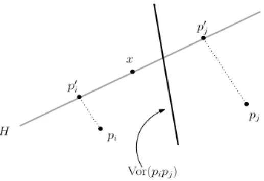
pi pj x p′ i p′ j H Vor(pipj)

Figure 1: Refer to Lemma 1. The red line denotes the k-dimensional plane H and the black line denotes Vorω(pipj).

(see Lemma 1). The other main reason is that some flat simplices named slivers can be removed from a Delaunay triangulation by weighting the vertices (see [14, 8, 13] and Section 4).

Lemma 1. Let H be a k-dimensional affine space of Rd. The restriction of the weighted Voronoi diagram of_{P to H} is the k-dimensional weighted Voronoi diagram of_P′ _where

P′ _{is the orthogonal projection of}

P onto H and the squared

weight of p′iis ω2(pi)− kpi− p′ik2.

Proof. By Pythagoras theorem, we have ∀ x ∈ H ∩

Vorω_(p

i), kx − pik2− ω2(pi)≤ kx − pjk2− ω2(pj)⇔ kx −

p′

ik2+kpi− pi′k2− ω2(pi)≤ kx − p′jk2+kpj− p′jk2− ω2(pj),

where p′

i denotes the orthogonal projection of pi ∈ P onto

H. Hence the restriction of Vorω₍

P) to H is the weighted Voronoi diagram of the weighted points (p′

i, ωi)∈ H where

ω2

i =−kpi− p′ik2+ ω2(pi).

Lemma 2 ([13]). If τ is a simplex of Delω(P), then

1. _{∀z ∈ aff(Vor}ω_{(τ )) and} ∀ p, q ∈ τ we have kq − zk ≤ kp−zk √_1−4ω2 0 . 2. Rτ ≤ R ′ τ √_1−4ω2 0 . 3. _{∀z ∈ aff(Vor}ω_{(τ )) and} ∀p ∈ τ , rz=pkp − zk2− ω2(p) ≥ R′ τ.

2.2

Sampling conditions

2.2.1

Local feature size

The medial axis of M is the closure of the sets of points of Rdthat have more than one nearest neighbor on M. The

local feature size of x_{∈ M, lfs(x), is the distance of x to the}

medial axis of M. As is well known and can be easily proved, lfs is Lipschitz continuous i.e, lfs(x)≤ lfs(y) + kx − yk.

2.2.2

-sample

The point sample_{P is said to be an (ε, δ)-sample (where} 0 < δ < ε < 1) if (1) for any point x∈ M there exists a point p_{∈ P such that ||x − p|| ≤ ε lfs(x), and (2) for any} two distinct points p, q_{∈ P, ||p − q|| ≥ δ lfs(p).}1 _{The ratio}

ε/δ is called the relative density ofP.

1_{Observe that the sparsity condition (2) is mandatory if one}

wants to infer the dimension of M from a sample [22].

We will use the following results from [22]. We write lp

for the distance between p_{∈ P and its nearest neighbor in} P \ {p}.

Lemma 3. Given an (ε, δ)-sampleP of M, we have

1. δ lfs(p)_{≤ l}p≤_1−ε2εlfs(p).

2. For any two points p, q_{∈ M such that ||p−q|| = t lfs(p),}

0 < t < 1, sin ∠(pq, Tp)≤ t/2.

3. Let p be a point in M. Let x be a point in Tpsuch that

||p − x|| ≤ t lfs(p) for some 0 < t ≤ 1/4. Let x′ _{be the} point on M closest to x. Then||x − x′

|| ≤ 2t2_lfs(p).

2.3

Slivers and good simplices

Consider a j-simplex τ , where 1 _{≤ j ≤ k + 1. We} de-note by Rτ, Lτ, Vτ and ρ(τ ) = Rτ/Lτ the circumradius, the

shortest edge length, the volume, and the radius-edge ratio of τ respectively. We further define σ(τ ) =`Vτ/Ljτ

´1/j , as the sliverity measure of τ . The orthocenter of τ is denoted by oτ and its orthoradius by R′τ.

If p_{∈ τ , we define τ}p= τ\ {p} to be the (j − 1)-face of

τ opposite to p. We also write Dτ(p) for the distance from

p to the affine hull of τp, and Hτ(p) for the signed distance2

from oτ to aff(τp). We state without proof the following

easy lemma.

Lemma 4. Let τ be a simplex of Delω₍

P) and p ∈ τ s.t.

1. There exists z_{∈ aff(Vor}ω_{(τ )) s.t.}

kz − pk ≤ L1. 2. _{kp − qk ≤ L}2 for all vertices q of τ .

3. R′

τ ≤ γ0Lτ.

Then_|Hτ(x)| = dist(oτ, aff(τx))≤ L1+ (1 + γ0+ ω0)L2 for all vertices x of τ .

Lemma 5 ([13]). Let τ be a simplex of Delω₍

P). Let p

be any vertex of τ and write Hτ(ω(p)) (instead of Hτ(p)) for the signed distance of oτ to aff(τp) parametrized by the weight of p. We have Hτ(ω(p)) = Hτ(0)− ω

2

(p) 2Dτ(p).

Slivers are a special type of flat simplices. The property of being a sliver is measured in terms of a parameter σ0, called

the sliverity bound, to be fixed later in Section 4.

Definition 1 (Sliver). Given a positive parameter σ0, slivers are defined by induction on the dimension : (1) a sim-plex of dimension less than 3 is not a σ0-sliver, and (2) for

j_{≥ 3, a j-simplex τ is a σ}0-sliver if σ(τ ) < σ0and,∀τ′⊂ τ ,

σ(τ′)≥ σ0.

Lemma 6. If a j-simplex τ is a σ0-sliver, then Dτ(p) <

jσ0Lτ for all vertices p∈ τ .

Proof. The volume of τ is Vτ = Vτp. Dτ(p) j = σj−1_(τ p)Lj−1τp . Dτ(p) j

and it is also equal to σj(τ )Ljτ. Since τ is a σ0-sliver, we

have σ(τ ) < σ0 and σ(τp)≥ σ0. Therefore we get

Dτ(p) = j σ j_{(τ )} σj−1_(τp)× Ljτ Lj−1τp < jσ0Lτ. 2_{H(p) is positive if o}

τ ∈ aff(τ ) and p lie on the same side

of aff(τp), and it is negative if they lie on different sides of

Vor(pq) Vor(pr) p r q Tp M

Figure 2: [pq] and [pr] are edges of the star of p in Delω

T M(P) since their dual Voronoi edges intersect the

tangent space Tp at p.

Definition 2 (Good simplex). Given two positive

con-stants ρ0and σ0, a simplex τ is called a (ρ0, σ0)-good simplex if ρ(τ )_{≤ ρ}0 and τ nor its subsimplices are σ0-slivers.

The following important lemma is known (see e.g. [14]). Lemma 7 (Normal approximation). Let τ be a (ρ0, σ0 )-good j-simplex for j _{≤ k with vertices on a k-dimensional} smooth manifold M, and p∈ τ s.t. the lengths of the edges

of τ that are incident to p are less than c3εlfs(p) for c3ε < 1. Then, for any normal vector np of M at p, τ has a normal

nτ such that ∠npnτ ≤ αj(σ0)ε where αj(σ0) depends on j,

σ0, ρ0 and c3, and 1/αj(σ0) vanishes with σ0.

In the sequel, we will simply write α(σ0) for αk(σ0).

2.4

Tangential Delaunay complex and

incon-sistent configurations

Let Delωpi(P) be the weighted Delaunay triangulation of

P restricted to the tangent space Tpi. Equivalently, the

simplices of Delω

pi(P) are the simplices of Del

ω₍

P) whose Voronoi dual faces intersect Tpi, i.e. τ ∈ Del

ω

pi(P) iff Vor

ω_{(τ )}

∩ Tpi 6= ∅. Observe that Del

ω

pi(P) is in general a k-dimensional

triangulation. Since this situation can always be ensured by applying some infinitesimal perturbation on _{P, we will} assume, in the rest of the paper, that all Delωpi(P) are

k-dimensional triangulations. Finally, write star(pi) for the

star of piin Delωpi(P), i.e. the set of simplices that are

inci-dent to piin Delωpi(P).

We call tangential Delaunay complex or tangential com-plex for short, the simplicial comcom-plex _{{τ, τ ∈ star(p), p ∈} P}. We denote it by Delω

T M(P). By our assumption above,

Delω

T M(P) is a k-dimensional complex contained in Delω(P).

By duality, computing star(pi) is equivalent to computing

the restriction of the (weighted) Voronoi cell of pi to Tpi,

which, by Lemma 1, reduces to computing a cell in a k-dimensional weighted Voronoi diagram embedded in Tpi. It

follows that the tangential complex can be computed with-out constructing any data structure of dimension higher than k, the intrinsic dimension of M.

The tangential Delaunay complex is not in general a tri-angulated manifold and therefore not a good approximation of M. This is due to the presence of so-called inconsisten-cies. Consider a k-simplex τ of Delω

T M(P) with two vertices

piand pjsuch that τ is in star(pi) but not in star(pj) (refer

to Fig. 3). We write Bi(τ ) for the open ball centered on

Tpi that is orthogonal to the (weighted) vertices of τ

ω_{, and} pi cpi cpj pj Tpi Tpj iφ ∈Vor(pl) ∈Vor(pipj) M ∈Vor(pipjpl)

Figure 3: An inconsistent configuration in the un-weighted case. Edge [pipj] is in Delpi(P) but not in

Delpj(P) since Vor(pipj) intersects Tpi but not Tpj.

This happens because [cpicpj] penetrates (at iφ) the

Voronoi cell of a point pl6= pi, pj, therefore creating

an inconsistent configuration φ = [pi, pj, pl].

denote by cpi and rpi its center and its radius. According

to our definition, τ is inconsistent iff Bi(τ ) is further than

orthogonal from all weighted points in Pω

\ τω _{while there}

exists a weighted point of _Pω

\ τω_{, say p}ω

l, that is closer

than orthogonal from Bj(τ ). We deduce from the above

discussion that the line segment [cpicpj] has to penetrate

the interior of Vorω_(p l).

We formally define an inconsistent configuration as fol-lows.

Definition 3 (Inconsistent configuration). φ = [p1

, . . . , pk+2] is called an inconsistent configuration of DelωT M(P) witnessed by the triplet (pi, pj, pl) if

• The k-simplex τ = φ \ {pl} is in star(pi) but not in

star(pj).

• τ is a (ρ0, σ0)-good simplex.

• Vorω_(p

l) is the first cell of Vorω(P) whose interior is intersected (at a point denoted by iφ) by the line seg-ment [cpicpj] oriented from cpi to cpj. Here cpi =

Tpi∩ Vor

ω_{(τ ) and c}

pj = Tpj∩ aff(Vor

ω_{(τ )).}

Note that iφis the center of a sphere that is orthogonal to

the weighted vertices of τ and also to pωl, and further than

orthogonal from all the other weighted points of_Pω_.

Equiv-alenty, iφis the point on [cpicpj] that belongs to Vor

ω_(φ).

An inconsistent configuration is thus a (k + 1)-simplex of Delω₍

P). Such a configuration or its subfaces do not necessarily belong to Delω

T M(P)3 We write Inω(P) for the

subcomplex of Del(_{P) consisting of all the inconsistent} con-figurations of Delω_{T M}(P) and their subfaces.

3.

STRUCTURAL RESULTS

In the rest of the paper, we will need several constants : ω0, ρ0 and σ0 (to define slivers, good simplices and

incon-sistent configurations), and c3 (to be able to use lemma 7). 3_{In fact, as already noted, no (k + 1)-simplex belongs to}

Delω

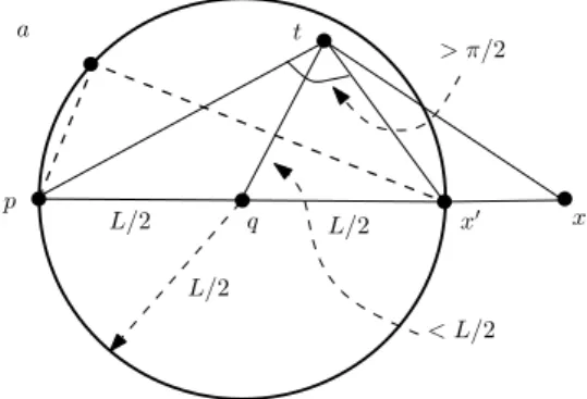
p a q t x′ x L/2 L/2 L/2 < L/2 > π/2

Figure 4: Refer to Lemma 8. x′_{is a point on the line}

segment such that _{||p − x}′

|| = c1ε lfs(p), L = c1ε lfs(p),

∠pax′= π/2 and ∠ptx≥ ∠ptx′> π/2.

These constants will be fixed in Section 3 and in Section 4. For simplicity, we will write sliver for σ0-sliver and

inconsis-tent configuration for (ρ0, σ0)-inconsistent configuration.

We give now an hypothesis which is assumed to be satis-fied in the following results.

Hypothesis 1. _{P is an (ε, δ)-sample of M of bounded}

relative density, i.e. ε/δ ≤ η0 for some positive constant

η0. We assume further that ε is small enough and that

2α(σ0)ε < 1. Finally, we assume that ˜ω ≤ ω0 where ˜ω is the relative amplitude of the weight assignement ω and ω0 is a positive constant less than 1/2.

3.1

Properties of the tangential Delaunay

com-plex

We now give the following two lemmas which are slight variants of results of [14].

Lemma 8. For all x∈ Tp∩Vorω(p), there exists a positive constant c1 such that||p − x|| ≤ c1εlfs(p).

Proof. Assume for a contradiction that there exists a point x∈ Vorω_(p)

∩ Tps.t. ||p − x|| > c1εlfs(p) with c1(1−

c1ε) > 2 + c1ε(1 + c1ε) (*). Let q be a point on the line

segment [px] such that_{||p − q|| = c}1εlfs(p)/2. Let q′be the

point nearest to q on M. From Lemma 3, we have||q −q′

|| ≤ c2 1ε2lfs(p)/2. Hence,_{||p − q}′ || ≤ ||p − q|| + ||q − q′ || < c1 2 ε(1 + c1ε)lfs(p).

From the 1-Lipschitz property, lfs(q′)_{≤ lfs(p) + ||p − q}′_{|| <} (1 +c1

2 ε(1 + c1ε)) lfs(p) < c1

2(1− c1ε) lfs(p), which yields

||p − q′|| ≥ ||p − q|| − ||q − q′|| > c₂1ε(1_{− c}1ε) lfs(p)

Since P is an ε-sample, there exists a point t ∈ P, s.t. ||q′ − t|| ≤ εlfs(q′_{) <} c1 2ε(1− c1ε) lfs(p). We thus have ||q − t|| ≤ ||q − q′ || + ||q′ − t|| < c₂1εlfs(p).

From Fig. 4, we can see that ∠ptx > π/2. This implies that_{||x − p||}2_{− ||x − t||}2_{− ||p − t||}2> 0. Hence, ||x − p||2 − ||x − t||2− ω2(p) + ω2(t) ≥ ||p − t||2− ω2(p) ≥ ||p − t||2 − ω2 0.||p − t||2 > 0 (as ω0<1₂)

This implies x6∈ Vorω_{(p), which contradicts our initial}

as-sumption. We conclude that Vorω_(p)

∩Tp⊆ B(p, c1εlfs(p)) if

Inequality (*) is satisfied, which is true for all c1 = 3 +√2≈

4.41 and ε < 0.09.

Lemma 9. There exists positive constants c2 and ρ′0 s.t. 1. If pq is an edge of Delω

T M(P), then ||p − q|| ≤ c2εlfs(p). 2. If τ is a simplex of Delω

T M(P), then R′τ ≤ ρ′0Lτ and

ρ(τ ) = Rτ/Lτ ≤ ρ′0.

Proof. 1a. Consider first the case where pq is an edge of Delω

p(P). Then Tp∩ Vorω(pq)6= ∅. Let x ∈ Tp∩ Vorω(pq).

From Lemma 8, we have||p − x|| ≤ c1εlfs(p). By Lemma 2,

||q − x|| ≤ √kp−xk 1−4ω2 0 ≤ c1εlfs(p) √ 1−4ω2 0 . Hence, kp − qk ≤ c′ 2εlfs(p) where c′ 2= c1(1 + 1/p1 − 4ω02) > 2c1.

1b. From the definition of Delω

T M(P), there exists a vertex

r of τ such that [pq]_{∈ star(r). From 1a, kr − pk and kr − qk} are at most c′

2εlfs(r). From the 1-Lipschitz property of lfs

and assuming that 2c′

2ε < 1, we have lfs(r)≤ lfs(p) + kp −

r_{k ≤ 1−c}lfs(p)′

2ε ≤ 2 lfs(p). It follows that kp − qk ≤ kp − rk +

kr − qk ≤ 4c′

2εlfs(p). The first part of the lemma is proved

by taking c2= 4c′2 > 8c1.

2. Assume that τ _{∈ star(p). Let z ∈ Vor}ω_{(τ )}

∩ Tp, and

rz =p||z − p||2− ω2(p). By definition, the ball centered at

z with radius rz is orthogonal to the weighted vertices of τ .

From Lemma 2, we have rz ≥ R′τ. Hence it suffices to prove

rz ≤ ρ′0Lτ. Since z∈ Vorω(τ )∩ Tp, we deduce from Lemma

8 that_{||z − p|| ≤ c}1εlfs(p). Therefore

rz=p||z − p||2− ω2(p)≤ ||z − p|| ≤ c1εlfs(p).

For any vertex q of τ , we have _{kp − qk ≤ c}2εlfs(p) (By

1.). Assuming 2c2ε ≤ 1 and using the fact that lfs is

1-Lipschitz, lfs(p)≤ 2lfs(q). Therefore, taking for q a vertex of the shortest edge of τ , we have, using Lemma 3,

rz ≤ c1 “ε δ ” δ lfs(p)≤ c1 “ε δ ” δ × 2lfs(q) ≤ 2c1η0Lτ = ρ′′0Lτ.

From Lemma 2, we have Rτ ≤ R

′ τ √ 1−4ω2 0 . Therefore ρ(τ )_≤ ρ′ 0= ρ′′ 0 √ 1−4ω2 0 .

3.2

Properties of inconsistent configurations

We now give the lemmas on inconsistent configurations which are central to the proof of correctness of the recon-struction algorithm given later in the paper.

Lemma 10. Let φ ∈ Inω₍

P) be an inconsistent

configu-ration witnessed by (pi, pj, pl). Then, there exists positive constants c3> c2 and ρ0> ρ′0 s.t.

1. _{kp − i}φk ≤c₂3εlfs(p) for all vertices p of φ. 2. If pq is an edge of φ thenkp − qk ≤ c3ε lfs(p). 3. If τ is a j-dimensional face of φ (j ≤ k + 1) and R′

τ is the orthosphere of τ , then R′

τ ≤ ρ0Lτ and Rτ/Lτ ≤

ρ0.

Proof. From the definition, τ = φ_{\ {p}l} belongs to

Delω

oτ is the orthocenter of τ . By Lemma 8, kpi− cpik ≤

c1εlfs(pi) and, by Lemma 2, we have

kpj− cpik ≤ kpi− cpik p1 − 4ω2 0 ≤ c1ε lfs(pi) p1 − 4ω2 0

Let c3= c2/p1 − 4ω02> c2. By Lemma 7, ∠(aff(τ ), Tpi)≤

α(σ0) ε, which implies that sin ∠(aff(τ ), Tpi)≤ α(σ0)ε and

tan2∠(aff(τ ), Tpi)≤ α2_(σ 0) ε2 1_{− α}2_{(σ0) ε}2 < 4 α 2_(σ 0) ε2,

since 2α(σ0)ε < 1 (Hypothesis 1). Observing that ||pi−

oτ|| ≤ ||pi−cpi||, since oτbelongs to aff(Vor

ω_{(τ )) and}

there-fore is the closest point to pi in aff(Vorω(τ )), we deduce

kcpi− oτk ≤ kcpi− pik sin ∠(aff(τ ), Tpi)≤ α(σ0)c1ε

2_lfs(p i).

Moreover,_||pj−oτ|| ≤ ||pj−cpi|| as oτ is the closest point

to pjin aff(Vorω(τ )). Hence we have,

kcpj− oτk ≤ kpj− oτk tan ∠(aff(τ ), Tpj) < 2 α(σ0) c1ε 2 p1 − 4ω2 0 lfs(pi) As iφ∈ [cpicpj], we conclude that koτ− iφk ≤ 2 α(σ0) c1ε2 p1 − 4ω2 0 lfs(pi).

1. Assuming that 2α(σ0) ε < 1 and using the facts that

kpi− oτk ≤ kpi− iφk, we get kpi− iφk ≤ kpi− oτk + koτ− iφk ≤ kpi− cpik + koτ− iφk ≤ c1ε +2α(σ0)c1ε 2 p1 − 4ω2 0 ! lfs(pi) ≤ c₄2 εlfs(pi)

From Lemma 2, we have _{kp − i}φk ≤ kpi−iφk √ 1−4ω2 0 = c3 4 εlfs(pi)

for all vertices p of φ.

2. Using part 1 of this lemma, we have kp − qk ≤ kp − iφk + kq − iφk ≤

c3

2 εlfs(pi) Moreover, lfs(pi)≤ 2lfs(p) since lfs is a 1-Lipschitz function

and by taking c3ε < 1. Hence kp − iφk ≤ c₂3εlfs(p) and

kp − qk ≤ c3ε lfs(p).

3. Let rφ =pkiφ− pik2− ω2(pi). Since iφ ∈ Vorω(τ ),

the ball centered at iφ with radius rφ is orthogonal to the

weighted vertices of τ . From Lemma 2, we have rφ≥ R′τ.

Hence it suffices to show that rφ≤ ρ0Lτ. Usingkpi− iφk ≤ c3

4 εlfs(pi) we get

rφ=pkiφ− pik − ω2(pi)≤ kiφ− pik ≤

c3

4 εlfs(pi). Let q be a vertex of a shortest edge of τ . We have, from part 2 of this lemma,_kpi− qk ≤ c3εlfs(q). Therefore

R′τ ≤ rφ≤ c3εlfs(q)≤ c3

“ε δ ”

δ_{× lfs(q) ≤ c}3η0Lτ

From Lemma 2, we have Rτ ≤ Rτ′/p1 − 4ω02. Therefore ,

Rτ/Lτ ≤ ρ0= c3η0/p1 − 4ω02.

Lemma 11. Let τ be a j-simplex of Delω_{T M}(P) ∪ Inω₍

P), j _{≤ k + 1. For any vertex p of τ , there exists a constant} c4 s.t. the distance between the orthocenter o(τ ) of τ and

aff(τp) is at most c4εlfs(p).

Proof. 1. We first consider the case where τ _{∈ In}ω₍

P). Then there exists an inconsistent configuration φ witnessed by points (pi, pj, pl) s.t. τ is a j-dimensional subsimplex of

φ. From Lemma 10, we have_kiφ− pk ≤c₂3εlfs(p),kq − pk ≤

c3lfs(p) for all q∈ φ and, since τ ∈ Inω(P), ρ(τ ) ≤ ρ0. Using

the above facts and Lemma 4, we get dist(oτ, aff(τp)) ≤ dist(iφ, aff(τp))

≤ c₂3εlfs(p) + (1 + ρ0+ ω0)c3lfs(p)

≤ (3₂+ ρ0+ ω0)c3εlfs(p) = c4εlfs(p),

2. Consider now the case where τ ∈ Delω

T M(P). By

def-inition, τ _{∈ Del}ω

q(P) for some vertex q of τ . From Lemma

8, we have _{kq − c}qk ≤ c1εlfs(q) ≤ 2c1εlfs(p) where cq =

Vorω(τ )_∩Tqand p is any vertex of τ . The last inequality

fol-lows from the facts that lfs is 1-Lipschitz,_{kp−qk ≤ c}2εlfs(p)

(Lemma 9) and by taking c2ε≤ 1. Therefore, using Lemma

4, we get dist(oτ, aff(τp)) ≤ 2c1εlfs(p) p1 − 4ω2 0 + (1 + ρ′0+ ω0)c2εlfs(p).

The next lemma shows that inconsistent configurations are slivers provided that σ0is sufficiently large wrt ε.

Lemma 12. Let φ be an inconsistent configuration and ε < f(σ0) =

(k + 1) σ0

ρ0(c3 + 2 α(σ0))

.

If the subfaces of φ are not slivers, then φ is a sliver.

Proof. Let pq be the smallest edge of φ and let r be a vertex in φ_{\ {p, q}. Since φ}r= φ\ {r} is not a sliver (as all

subfaces of φ are not slivers) and_{kr − xk ≤ c}3lfs(x) (Lemma

10), we have sin ∠(aff(φr), Tx) ≤ α(σ0) ε for all vertices x

of φr by Lemma 7. From Lemma 3, sin ∠(pr, Tp) ≤ c₂3ε.

Therefore

Dφ(r) = sin ∠(pr, aff(φr))× kp − rk

≤ (sin ∠(pr, Tp) + sin ∠(aff(φr), Tp))× kp − rk

≤ (c₂3 + α(σ0)) εkp − rk.

Using the facts that vol(φr) = σk(φr) Lφkr, σ(φr)≥ σ0,kp −

rk ≤ 2Rφ, ρ(φr)≤ ρ0 and ε < f(σ0), we get vol(φ) = Dφ(r)×vol(φr) k + 1 ≤ “c₂3 + α(σ0) ” εkp − rk ×σ k_(φ r)Lkφ k + 1 ≤ (c3+ 2α(σ0)) εRφ× σk 0Lkφ k + 1 ≤ ρ0(c3+ 2α(σ_{k + 1} 0))ε× σ0kLk+1φ < σk+10 Lk+1φ

3.3

Number of local neighbors

Lemmas 9 and 10 show that, in order to construct star(p) and search for inconsistencies involving p, it is enough to consider the points ofP that lie in ball Bp= B(p, c3εlfs(p)).

Since ε and lfs(p) are not known in practice, we will consider instead the ball B′

p= B(p, c3η0lp) where

lx= min

q∈P,q6=xkx − qk.

It is easily seen that lx : M → R is 1-Lipschitz and, by

Lemma 3, we have δlfs(p)≤ lp≤ _1−ε2ε lfs(p). It follows that

Bp′ contains Bpif ε/δ≤ η0. We call LNp= B′p∩ P the local neighborhood of p.

Lemma 13. The number of points of LNp is less than

N < 2O(k)_.

Proof. For convenience, write ν = 4c3η0ε and assume

that ν≤ 1/2. We observe that LNp ⊂ B′′p = B(p, νlfs(p))

since, by Lemma 3, lp≤_1−ε2ε lfs(p)≤ 4εlfs(p). We will count

the number of points in B′′

p∩ P. Let x and y be two points

of B′′

p∩ P. We have lfs(x), lfs(y) ≥ lfs(p)(1 − ν) ≥ lfs(p)/2,

since lfs is 1-Lipschitz. The balls B(x, lx/2) and B(y, ly/2)

are disjoint, and, since lx≥ δ lfs(x) ≥ δ₂lfs(p) (and similarly

for ly), the balls Bx= B(x,δ₄lfs(p)) and By= B(y,δ₄lfs(p))

are also disjoint. Observe that both balls Bx and By are

contained in B+

p = B(p, µ εlfs(p)) where µ = νε + δ 4ε ≤

4c3η0+1₄.

A packing argument now allows to conclude. Specifically, by Lemma 15, we have that vol(Bx∩ M) > φk

“

δ lfs(p) 8

”k and vol(Bp+∩ M) < φk(µεlfs(p))k, where φk is the volume

of the k-dimensional unit ball. We conclude that the number of points of_{P ∩ B}′′p is less than

`8µε δ ´k ≤ (32c3η0+ 2)kη0k= 2O(k).

4.

MANIFOLD RECONSTRUCTION

In this section, we will show how to find a weight as-signment for the point set_{P so that we can remove all} in-consistent configurations. Once this is done, all the stars become coherent and the resulting weighted tangential De-launay complex is a simplicial k-manifold.

4.1

Algorithm

The input to the algorithm is a point sample_{P = {p}1, . . . , pn}

together with a bound on the relative density η0 ofP. We

assume in addition that the dimension k of M is given and that we know the tangent space Tpat each point p∈ P.

The algorithm fixes ω0 in (0, 1/2) and then computes a

weight assignment ω_{∈ [0, ω}0] such that no inconsistent

con-figuration remains in the weighted tangential Delaunay com-plex. More precisely, we will assign a weight to each point p_{∈ P in turn so as to remove all j-dimensional slivers} in-cident to p in Delω_{T M}(P) ∪ Inω₍

P) for j ∈ {3, . . . , k + 1}. By Lemma 12, we know that, if σ0 is large enough,

remov-ing inconsistent configurations from the tangential Delaunay complex reduces to removing slivers.

For a given j-simplex τ = [p0, . . . , pj] ∈ Delω_{T M}(P) ∪

Inω₍ P) we have σj(τ ) = | det(p1− p0, . . . , pj− p0)| j! Ljτ ≤ Π j i=1kpi− p0k j! Ljτ ≤ 2jρj₀ j! ≤ 2ρ j 0,

the last inequalities follow from the facts that Lτ ≤ 2 Rτ,

and the radius-edge ratio of the simplices in Delω T M(P) ∪

Inω₍

P) is ≤ ρ0(Lemmas 9 and 10). This implies that σ(τ )∈

(0, 2 ρ0]. In the first step of our reconstruction algorithm,

we pick a random value of σ0from (0, 2ρ0], and once σ0is

se-lected, we try to remove all slivers from Delω

T M(P) ∪ Inω(P).

If we fail to remove slivers or if we still have inconsistencies, then we go back and select a new value of σ0.

Manifold-Reconstruction(_{P = {p}1, . . . , pn})

S0 Calculate LNpi∀pi∈ P and ρ1

S1 Select σ0 at random from (0, 2 ρ1]

S2 for i = 1 to n do

if weight(pi, σ0) = “FAIL” then go-to S1

else update(Delω

T M(P), pi)

S3 if Inω₍

P) 6= ∅ then go-to S1 else output Delω

T M(P)

Before we give the details of the function weight() we first define the subroutine skyline(p, S, σ0) that will be used in

the function. Let S be a set of simplices incident on p. Let τ be a simplex in S whose subfaces are not σ0-slivers.

Such a simplex is called a candidate simplex. We associate to τ interval W (τ ) that consists of all squared weights ω2_(p)

for which τ appears as a simplex in Delω

T M(P) ∪ Inω(P). We

define the skyline of p as the lower boundary of the union of all rectangles R(τ ) = W (τ )_{× [σ(τ ), +∞) for all} candi-date simplices over W (p) = [0, ω2

0l2p], see Figure 5. For any

ω2(p), the minimum sliverity ratio of any candidate

sim-plex incident to p is the height of skyline(p, Sp, σ0) over

ω2_(p)

∈ W (p). The best choice for ω(p) is the weight of p corresponding to the highest point on the skyline(p, Sp, σ0),

i.e skyline(p, Sp, σ0) has the maximum height over ω2(p).

Function weight(p, σ0)

S1 Sp← detect simplices(p, σ0)

S2 skyline(p, Sp, σ0) begin

for i = 1 to n do

if none of the subfaces of τ are σ0-slivers then

include R(τ ) = W (τ )_{× [σ(τ ), +∞)} end

S3 Θ← highest point on skyline(p, Sp, σ0)

S4 if Θ < σ0 then return “FAIL”

else ω(p)← weight of p corresponding to a highest point on skyline(p, Sp, σ0)

Function update(Delω

T M(P), p)

− Update the stars of p and of all points x ∈ LNp by

modifying Delω x(LNx).

Function detect simplices(p, σ0)

1. We first detect all possible j-simplices for all 3_{≤ j ≤} k + 1 of Delω_{T M}(P) incident on p for all possible ω(p). This is done in the following way: (1) we vary the weight of p from 0 to to ω0lp, keeping the weights of

the other points constant; (2) for each new weight as-signment to p, we modify the stars of the points in LNp

ω2 0l 2 p W(p) 0

Figure 5: The above figure shows a skyline(p, Sp, σ0)

over W (p) = [0, ω2_l2

p] for point p.

to p that have not been detected thus far. The weight of point p changes only in a finite number of instances 0 = P0 < P1<· · · < Pn−1< Pn= ω0lp.

We determine the next weight assignment of p in the following way. For each new simplex τ currently inci-dent to p, we keep it in a priority queue ordered by the weight of p at which τ will disappear for the first time. Hence the minimum weight in the priority queue gives the next weight assignment for p. Since the number of points in LNpis bounded, the number of simplices

incident to p is also bounded, as well as the number of times we have to change the weight of p.

2. Once we have detected all possible j-simplices, for all j ∈ {1, . . . , k + 1}, that can be incident on p in the weighted tangential Delaunay complex, we then de-tect all possible inconsistent configurations incident on p, by calling the function detect inconsistent-configuration(p, σ0).

Function detect inconsistent-configurations(p, σ0)

1. We vary the weight of p from 0 to ω0lp, keeping the

weight of the rest of the points constant. Once we have assigned a new weight to p we modify the stars of the points in LNp.

2. Detecting the inconsistent configurations incident to p is more complicated than detecting the simplices inci-dent to p. We consider all points pi in LNp. Let τ be

a k-simplex in the star of pi, and let pj be a vertex

of τ such that τ is not in the star of pj. We calculate

the Voronoi diagram of the points in LNprestricted to

the line segment [cpicpj], where cpi = Tpi∩ Vor

ω_{(τ )}

and cpj = Tpj ∩ aff(Vor

ω_{(τ )). From the restricted}

Voronoi diagram, we find a point p whose Voronoi cell intersects for the first time the line segment [cpicpj]

oriented from cpi to cpj. If p∈ φ = τ ∪ {l}, then we

report φ.

3. As in the detect simplices function the weight of p is changed only a finite number of times. For each current inconsistent configuration φ incident to p, we keep in a priority queue the weight of p for which φ will disappear for the first time. The minimum weight in the priority queue gives the next weight assignment of p.

4.2

Analysis of the algorithm

Definition 4 (Sliverity range). Let ω be a weight

assignment of relative amplitude at most ω0 we keep fixed

except for ω(p). The sliverity range of a point p∈ P is the

measure of the set of all squared weights ω2_{(p) for which p} is incident to a sliver in Delω

T M(P) ∪ Inω(P).

Lemma 14. Under Hypothesis 1, the sliverity range of p

is at most Σ(p) = Nk+2_{(k + 1)c}

5σ0l2pfor some constant c5.

Proof. Let τ be a simplex incident on p. We call the sliverity range of τ the measure of the set of squared weights for which τ is a sliver in Delω

T M(P) ∪ Inω(P). If ω(p) is

the weight of p, we write H(ω(p)) for the signed distance of the orthocenter of τ to aff(τp). From Lemma 11, we

have _{|H(ω(p))| ≤ c}4εlfs(p), for all τ ∈ DelωT M(P) ∪ Inω(P).

Moreover, using Lemma 5 and the fact that τ is a sliver, H(ω(p)) = H(0)₋ω_2D2(p)

p ≤ H(0) −

ω2

(p)

2jσ0Lτ. It follows that

the sliverity range of τ is at most 4jσ0Lτc4εlfs(p). Using

the facts that Lτ ≤ c3εlfs(p) (from Lemmas 9 and 10),

lfs(p) _{≤ l}p/δ and ε/δ ≤ η0, the sliverity range of τ is less

than 4jc3c4σ0η02l2p = j c5σ0l2p. By Lemma 13, the number

of j-simplices that are incident to p is at most Nj_{. Hence,}

the sliverity range of p is less that Σ(p) =

k+1

X

3

Njjc5σ0l2p≤ Nk+2(k + 1)c5σ0l2p.

Theorem 1. Under Hypothesis 1 and if σmax=

ω2 0

(k + 1) c5Nk+2

> σmin= inf{σ|ε < f(σ)}, then, for any σ0∈ [σmin, σmax], the above algorithm outputs

Delω

T M(P) without any slivers nor inconsistent configuration.

Proof. As in subroutine skyline(), let Sp denotes the

set of all possible simplices that can be incident on p in the complex Delω

T M(P) ∪ Inω(P) for all possible weight

assign-ments ω of relative amplitude ˜ω≤ ω0. By Lemma 14, the

sliverity range of p is less than Nk+2_{(k + 1)c}

5σ0l2p. If the

sliverity range of p is less than ω2

0l2p, the total range of all

possible squared weights, or, equivalently, if

σ0< σmax= ω

2 0

(k + 1) c5Nk+2

,

then we will be able to remove all slivers incident on p by selecting the highest point on the skyline.

If we select a value of σ0 in the interval (σmin, σmax],

Lemma 14 ensures that removing all j-dimensional slivers for all j _{∈ {3, . . . , k + 1} in Del}ω

T M(P) ∪ Inω(P) will also

re-sult in removing inconsistent configurations from Delω T M(P),

i.e. Inω(P) = ∅.

4.3

Time and space complexity

Theorem 2. The time complexity of the algorithm is O(d)_|P|2+1

λ× 2

O(k2

)+log d

|P|,

where λ = (σmax− σmin)/(2ρ0), and its space complexity is

2O(k2)+log d_|P|.

Proof. We only sketch the complexity analysis. See [7] for a detailed discussion. Step S0 of Manifold-Reconstruc-tion can easily be performed in O(d)_|P|2 _time.

We show now that the expected number of times Step S1 of ManifoldReconstruction is repeated is 1

λ. Indeed, for

any simplex τ_{∈ Del}ω

T M(P)∪Inω(P), we have σ(τ ) ∈ (0, 2ρ0].

Hence, the probability that, for the selected value of σ0,

the algorithm removes all slivers and inconsistencies is at least λ = (σmax− σmin)/(2ρ0). It follows that the expected

number of times S1 is performed is less than

∞

X

i=1

i(1_{− λ)}i−1λ = 1 λ.

The time complexities of functions update(Delω

T M(P), p),

detect simplices (p, σ0), and detect

inconsistent-confi-gurations(p, σ0) are 2O(k(k+log d)). Indeed, we need to

pro-ject|LNp| < N < 2O(k)points onto Tp, which costs O(kd)×

|LNp| = O(d) 2O(k) time. The Delaunay simplices that are

computed have their vertices in LNp and are of dimension

at most k + 1. Hence their number is 2O(k2). The basic op-erations (mainly in-sphere predicates) amount to evaluating signs of determinants of k_{× k matrices. The cost of such a} basic operation is O(k3). The total cost of both functions is thus O(d) 2O(k)+ O(k3) 2O(k2)= 2O(k2)+log d.

We deduce that the expected time complexity of Manifold-Reconstruction is O(d)|P|2₊1 λ× 2 O(k2 )+log d |P|.

We easily deduce from the above discussion that the total space complexity of the algorithm is

2O(k2)+log d_|P|. (2)

4.4

Topological and Geometric guarantees

We assume that the conditions of Theorem 1 are satisfied and denote by Delω_{T M}(P) the tangential complex output by our algorithm. Let π be the mapping that maps any point of Delω

T M(P) to its closest point on M. The proof of topological

correctness (see [7]) uses ideas from [1, 8, 11, 14].

Theorem 3. Under the conditions of Theorem 1, our

al-gorithm outputs Delω_{T M}(P) without any slivers and

inconsis-tent configurations, and Delω

T M(P) has the following proper-ties

• Bijection : The restriction of π to Delω

T M(P) is a bijection;

• Pointwise approximation : ∀x ∈ M, dist(x, π−1_(x))

= O(ε2lfs(x));

• Normal approximation : ∀x ∈ M, ∠NxNτ= O(ε),

where τ is a k-simplex of Delω

T M(P) containing the point π−1_(x),

• Topological correctness : π defines an isotopy

be-tween Delω_{T M}(P) and M.

Proof sketch. By Lemma 7, one can show that the maximum distance from a point of a simplex τ∈ Delω

T M(P)

to the closest point on M is O(ε2_{lfs(x)). It follows that the}

projection π that maps every point of τ to its closest point on M is injective: if we extend an open segment of length lfs(y) from every manifold point y in all normal directions to M, these segments do not intersect, and they can be used

as the fibers of a tubular neighborhood ˆM of M. Each point of such a segment has y as its unique closest neighbor on M. For small enough ε, the simplex τ is contained in ˆM. Thus, the mapping π defines an isotopy between τ and a corresponding manifold patch.

One can show that two k-simplices of Delω

T M(P) that share

a subface have normal spaces that differ by at most O(ε), and that the mapping π extends continuously across the subfaces. It follows that the projection π restricted to the two adjacent k-simplices is a homeomorphism that is invert-ible locally. (In topological terms, π : Delω_{T M}(P) → M is a covering map, if we can establish that it is surjective.) By assumption, on every component, there is at least one vertex of a simplex of Delω_{T M}(P). This ensures that π(Delω

T M(P))

contains that vertex, and since the mapping can be contin-ued locally, it follows that every component of S is covered at least once. It is now still possible that some component is covered more than once by π. This would imply that some sample point p_{∈ P is covered more than once. However, one} can show quite easily that no point p of Delω

T M(P) except p

itself has p as its closest neighbor on M.

It follows that the mapping π defines an ambient isotopy between Delω_{T M}(_{P) and M.}

5.

CONCLUSION

We have given the first algorithm that is able to recon-struct a smooth manifold in a time that depends only lin-early on the dimension of the ambient space. We believe that our algorithm is of practical interest when the dimen-sion of the manifold is small, even if it is embedded in a space of very high dimension. This situation is quite common in practical applications in machine learning.

The algorithm is rather simple. The basic ingredients we need are data structures for constructing weighted Delaunay triangulations in k-flats. We will report experimental results in a forthcoming paper.

We have assumed that dimension of M is known. If not, we can use algorithms given in [22, 15] to estimate the di-mension of M and the tangent space at each sample point. One interesting feature of our approach is that it is pretty robust and still works if we only have approximate tangent spaces at the sample points.

We have also assumed that we know an upper bound on the relative density η0 of the input sample P. Ideas from

[21, 8] may be useful to convert a sample to a subsample with a bounded relative density.

We forsee other applications of the tangential complex and of our construction each time computations in the tangent space of a manifold are required, e.g. for dimensionality reduction and approximating the Laplace Beltrami operator [5].

Finally, let us mention that removing inconsistencies among stars that have been computed independently is a useful paradigm that has already been used for maintaining dy-namic meshes [29] and generating anisotropic meshes [9]. We hope that this paper will motivate further applications.

6.

ACKNOWLEDGEMENTS

The authors thank the anonymous referees for their in-sightful comments, and Mariette Yvinec for helpful discus-sions.

7.

REFERENCES

[1] N. Amenta, S. Choi, T. K. Dey, , and N. Leekha. A simple algorithm for homeomorphic surface reconstruction. Intl. Journal of Computational

Geometry and Application, 12:125–141, 2002.

[2] F. Aurenhammer. Power diagrams: properties, algorithms and applications. SIAM J. Comput., 16(1), 1987.

[3] F. Aurenhammer and H. Edelsbrunner. An optimal algorithm for constructing the weighted voronoi diagram in the plane. Pattern Recognition, 17(2):251–257, 1984.

[4] M. Belkin and P. Niyogi. Laplacian eigenmaps and spectral techniques for embedding and clustering.

Advances in Neural Information Processing Systems,

2001.

[5] M. Belkin, J. Sun, and Y. Wang. Discrete laplace operator on meshed surfaces. In Proc. ACM Symp. on

Computational Geometry, 2008.

[6] J.-D. Boissonnat and J. Fl¨ototto. A coordinate system associated with points scattered on a surface.

Computer-Aided Design, 36:161–174, 2004.

[7] J.-D. Boissonnat and A. Ghosh. Manifold

Reconstruction using Tangential Delaunay Complexes.

INRIA Research Report 7142, 2009.

[8] J. D. Boissonnat, L. Guibas, and S. Y. Oudot. Manifold reconstruction in arbitary dimensions using witness complexes. In Proc. ACM Symp. on

Computational Geometry, pages 193–204, 2007.

[9] J.-D. Boissonnat, C. Wormser, and M. Yvinec. Locally uniform anisotropic meshing. In Proc. ACM Symp. on

Computational Geometry, pages 270–277, 2008.

[10] F. Cazals and J. Giesen. Delaunay triangulation based surface reconstruction. In J. Boissonnat and

M. Teillaud, editors, Effective Computational

Geometry for Curve and Surfaces. Springer, 2006.

[11] F. Chazal and A. Lieutier. Smooth Manifold Reconstruction from Noisy and Non uniform Approximation with Guarantees. Comp. Geom:

Theory and Applications, 40:156–170, 2008.

[12] F. Chazal and S. Y. Oudot. Towards

Persistence-Based Reconstruction in Euclidean Spaces. In Proc. ACM Symp. on Computational Geometry, pages 232–241, 2008.

[13] S.-W. Cheng, T. K. Dey, H. Edelsbrunner, M. A. Facello, and S.-H. Teng. Sliver Exudation. Journal of

ACM, 47:883–904, 2000.

[14] S.-W. Cheng, T. K. Dey, and E. A. Ramos. Manifold Reconstruction from Point Samples. In Proc.

ACM-SIAM Symp. Discrete Algorithms, pages

1018–1027, 2005.

[15] S.-W. Cheng, Y. Wang, and Z. Wu. Provable Dimension Detection using Principle Component Analysis. Intl. Journal of Computational Geometry

and Application, 18(5):415–440, 2008.

[16] D. Cohen-Steiner and T. K. F. Da. A greedy Delaunay Based Surface Reconstruction Algorithm. The Visual

Computer, 20:4–16, 2004.

[17] T. K. Dey. Curve and Surface Reconstruction:

Algorithms with Mathematical Analysis. Cambridge

University Press, 2006.

[18] D. L. Donohu and C. Grimes. Hessian eigenmaps: new

locally linear embedding techniques for high

dimensional data. Proceedings of the Natural Academy

of Sciences, 100:5591–5596, 2003.

[19] J. Fl¨ototto. A coordinate system associated to a point

cloud issued from a manifold: definition, properties and applications. PhD thesis, Universit´e of Nice

Sophia-Antipolis, 2003.

[20] D. Freedman. Efficient simplicial reconstructions of manifolds from their samples. IEEE Trans. on Pattern

Analysis and Machine Intelligence, 24(10), 2002.

[21] S. Funke and E. Ramos. Smooth-surface reconstruction in near-linear time. In Proc.

ACM-SIAM Symp. Discrete Algorithms, pages

781–780, 2002.

[22] J. Giesen and U. Wagner. Shape dimension and intrinsic metric from samples of manifolds. In Proc.

ACM Symp. on Computational Geometry, pages

329–337, 2003.

[23] M. Gopi, S. Khrisnan, and C. T. Silva. Surface Reconstruction based on Lower Dimensional Localized Delaunay Triangulation. Eurographics, 19 (3), 2000. [24] S. Lafon and A. B. Lee. Diffusion Maps and

Coarse-Graining: A Unified Framework for

Dimensionality Reduction, Graph Partitioning, and Data Set Parameterization. IEEE Transactions on

Pattern Analysis and Machine Intelligence,

28:1393–1403, 2006.

[25] B. Nadler, S. Lafon, R. R. Coifman, and I. G. Kevrekidis. Diffusion maps, spectral clustering and eigenfunctions of fokker-planck operators. Neural

Information Processing Systems, 18, 2005.

[26] P. Niyogi, S. Smale, and S. Weinberger. Finding the Homology of Submanifolds with High Confidence from Random Samples. Discrete and Computational

Geometry, 39(1-3), March 2008.

[27] S. T. Roweis and L. K. Saul. Nonlinear dimensionality reduction by locally linear embedding. Science, 290:2323–2326, 2000.

[28] H. S. Seung and D. D. lee. The manifold ways of perception. Science, 290:2268–2269, 2000. [29] J. Shewchuk. Star splaying: An algorithm for

repairing delaunay triangulations and convex hulls. In

Proc. ACM Symp. on Computational Geometry, pages

237–246, 2005.

[30] J. B. Tenenbaum, V. deSilva, and J. C. Langford. A global geometric framework for nonlinear

dimensionality reduction. Science, 290:2319–2323, 2000.

[31] Z. Zhang and H. Zha. Principal manifolds and nonlinear dimension reduction via local tangent space alignment. SIAM Journal of Scientific Computing, 26(1):313–338, 2004.

APPENDIX

Lemma 15 ( [26]). Let A = B(p, r)_{∩ M where r ≤}

εlfs(M). Then, φkrk ≥ vol(A)φkrk/2k, where φk is volume of the k-dimensional unit ball.