HAL Id: hal-01103123
https://hal.inria.fr/hal-01103123v2
Submitted on 30 Jan 2015
HAL is a multi-disciplinary open access
archive for the deposit and dissemination of
sci-entific research documents, whether they are
pub-lished or not. The documents may come from
teaching and research institutions in France or
abroad, or from public or private research centers.
L’archive ouverte pluridisciplinaire HAL, est
destinée au dépôt et à la diffusion de documents
scientifiques de niveau recherche, publiés ou non,
émanant des établissements d’enseignement et de
recherche français ou étrangers, des laboratoires
publics ou privés.
Scale-Space Peak Picking
Antoine Liutkus
To cite this version:
Antoine Liutkus. Scale-Space Peak Picking. [Research Report] Inria Nancy - Grand Est
(Villers-lès-Nancy, France). 2015. �hal-01103123v2�
SCALE-SPACE PEAK PICKING
Antoine Liutkus
Inria, speech processing team, Villers-lès-Nancy, France
ABSTRACT
In this report, I present a peak detection method for 1D data, based on scale-space theory. Instead of focusing on local derivative information as is classical in peak detection, the proposed approach is more global. It performs iterative smoothings of the input data with increasing length-scales and then defines a peak as a datapoint that remains a local maximum for many such filterings. Formally, the local maxima are identified after each filtering operation and then associated to the maxima identified with the previous length-scales. A score is then added to the criterion for these latter points, that notably depends on the length-scale. This strategy enforces picks that remain local maxima even after many smoothing operations. At the end of the process, the peaks are identified as the points having the largest score. The approach is flexible enough to allow for different smoothing operations and different strategies for incrementing the score. I informally show on different kinds of signals that the proposed approach may be very effective, even for very noisy data.
I. INTRODUCTION
Peak-picking is an ubiquitous problem in signal pro-cessing. Whenever we have to detect the values for some phenomenon within a possibly large set of possibilities, we have to process to peak picking. A typical example is when analyzing spectra or distributions: among all possible values, the signal under study usually contains only a small number of active components. When doing analysis, we often have to detect which ones of those components are active and for this purpose, we need some peak detection algorithm. Although it is quite an easy problem to solve for the human eye, it definitely is a difficult problem to formalize. Its inherent difficulty is that on top of the target signal, or peaks, addi-tional information may be observed such as noise, drifting, linear or nonlinear trends, etc. Informally, detecting the peaks in a signal may be understood as identifying those points that clearly “stand out”, either from noise or from these “regular” background variations. However, such a definition is not amenable to a single quantitative interpretation and depending on the definition considered, peak picking may be achieved using very different paradigms. In this report, I only consider pick picking over one-dimensional signals such as time series or power spectra.
The most common peak picking methods used in practice involve the computation of empirical derivatives coupled with some criterion concerning the value of the signal. In that kind of methods, a peak is defined as a location where the signal is above some given absolute threshold, while its derivative — or some smoothed version of it— is crossing zero. Optionally, further criteria may be included, for instance enforcing that two peaks should not be too close together or that a peak should be surrounded by signal values much below it1.
Another route for designing peak picking methods is model-based. Simply put, the background signal is assumed to obey some particular model such as auto-regressive, and its parameters are fitted according to the data. The picks are then detected based on the quality of the data-fit: points that are not well explained by the model are categorized as peaks, and the criterion is given by the probabilistic interpretation. That approach has for instance been successfully applied on audio signals to detect cracking noise, see e.g. [4] for an overview of such probabilistic audio restoration methods.
In another vein, recent research has exploited multi-resolution representations to detect the peaks [3]. In this approach, the data first goes through a wavelet transform that is chosen so as to enhance the peaks and smooth out the background signal. Then, peaks across the scales are matched and their amplitude are summed so as to yield the final criterion on which detection is achieved. This idea of exploiting multiscale representations has proved very efficient to separate the peaks in many settings, notably in chemical engineering where it is a very important part of the processing of signals [1], [7].
In this report, I present a variation over the idea of ex-ploiting multiscale information to identify peaks as described in [3]. However, instead of framing it as a selection achieved in a multiscale representation, I rather adopt the scale-space paradigm detailed, e.g. in [5]. Scale-scale-space theory has attracted much attention in the image processing community because of its unique ability to automatically process the data at the adequate scale without having to manually tune many ad-hoc parameters. In a nutshell, it relies on smoothing the data using kernels (weighting windows) of various sizes, while performing processing on all those
1See for instance theFINDPEAKSmethod of Matlab http://fr.mathworks.
filtered versions jointly or iteratively. It has for instance been found very effective in estimating edges in images [6]. It is close in spirit to the celebrated Laplacian pyramid used to analyze or encode images by exploiting multi-scale features and redundancies [2]. The rationale for doing peak detection using scale-space theory is that we want to avoid explicitly informing the detection algorithm about the width or particular shape of the peaks, because we assume that this information is not known a priori. Integrating out this scale information through a consistent probabilistic treatment would of course be feasible, but relying on a ad-hoc scale-space processing yields a very computationally efficient method, which is sometimes a desirable property.
In this context, the approach I propose simply defines a peak as a point in the signal, which remains a local maximum in many scales. Doing so permits to avoid defining a peak based on its particular width or height, that may strongly vary across signals. Instead, local maxima along different scales are associated, which permits to increasingly build a criterion that summarizes their importance as peaks in many scales. Peak identification is simply achieved in the end by using this criterion.
This report is structured in the following way. In section II, I describe the peak detection function and in section III, I show some results of its usage on real data.
II. SCALE-SPACE PEAK PICKING
We assume the input data v is a vector of dimensions N × 1. Our objective is to detect the peaks in v. The Scale-Space Peak Picking method we propose (SSPP) is based on an iterative procedure that progressively builds a criterion C, which is itself a N × 1 vector, initialized to 0. At the end of the procedure, the decision is made based on C, totally ignoring the input data v for this purpose. Hence, C can be understood as a “peak presence function”, that is high whenever a peak is likely to be found.
First, all the local maxima of v are detected and stored in the set P. This is written:
P ← localmaxima (v) . (1) A sample index n is a local maximum if it is higher than its neighbours:
n ∈ localmaxima (v)
⇔ v (n) = max [v (n − 1) v (n) v (n + 1)] . (2) Since they were hence detected as local maxima, the points in P ought to see their criterion C incremented. For this reason, at the first iteration, we set:
∀p ∈ P, C (p) ← v (p) . (3) The rationale behind using v (p) in incrementing C is to promote points having a larger amplitude as peaks. The
selected peaks are also stored in a set O containing all previously selected peaks: O ← P.
At this stage, the signal v is smoothed using a small lengthscale s to yield a new smoothed version v. In practice, this is implemented by convolving v with a weighting window such as a normalized hamming window of length s. Then, local maxima are detected anew to yield the new set P as in (1) and (2). The main idea of the proposed SSPP technique is to associate these new local maxima to points in O that where already selected in previous iterations, and to to increment the criterion of these, because having them selected anew proves they are good candidates. This is achieved by first identifying which element of the old set O is closest to each element of P, thus building the set I of the neighbours of the elements of P:
∀p ∈ P, I (p) ← argmin o∈O
|p − o| .
When the neighbours I to current local maxima have been identified, the algorithm goes on by simply augmenting the corresponding criterion by some given amount, which for instance depends on both the signal value and the scale:
∀p ∈ P : ∆C(I (p)) ← v (I (p)) s2. (4) The rationale behind using s2 in expression (4) is to considerably promote points that remain peaks throughout successive smoothing, i.e. at increasing scales. Furthermore, the main advantage of incrementing the elements of I and not simply those of P is to avoid incrementing the criterion of different points at each iteration, which would inevitably happen because of the drifting that occurs between local maxima for different smoothing scales.
Finally, the procedure is iterated with a larger scale s. The process then increments the criterion C over the iterations, until some fixed set of increasing scales have been processed. At the end of the procedure, the peaks are identified as the points having either the largest C value (in case of a known number of peaks) or as the points whose criterion is larger than ρmax (C) with ρ ∈ ]0 1[.
The whole algorithm is summarized in alg. 1, and a free Matlab implementation is available online2.
III. RESULTS
Examples of usage of the proposed scale-space peak picking (SSPP) method are displayed for various kinds of signals in figure 1 (number of sunspots as a function of time), figure 2 (noisy sinusoidal signal) and figure 3 (impulsive peaks buried in noise). All those figures were generated with the free implementation of SSPP we propose for Matlab. Depending on the application, the user may know the number K of peaks to detect, or may rather have an approximate idea of the peak density, in which case, he can
2http://fr.mathworks.com/matlabcentral/fileexchange/
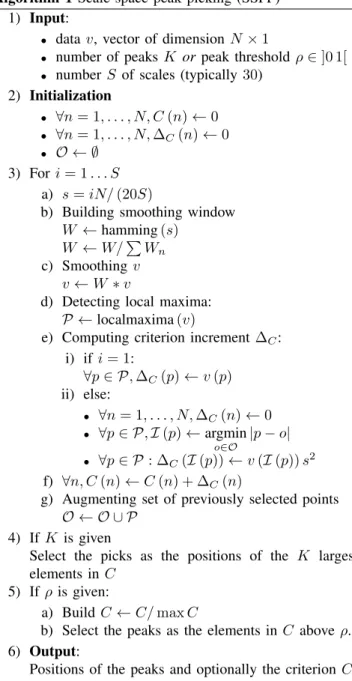
Algorithm 1 Scale-space peak picking (SSPP) 1) Input:
• data v, vector of dimension N × 1
• number of peaks K or peak threshold ρ ∈ ]0 1[ • number S of scales (typically 30)
2) Initialization • ∀n = 1, . . . , N, C (n) ← 0 • ∀n = 1, . . . , N, ∆C(n) ← 0 • O ← ∅ 3) For i = 1 . . . S a) s = iN/ (20S)
b) Building smoothing window W ← hamming (s)
W ← W/P Wn c) Smoothing v
v ← W ∗ v
d) Detecting local maxima: P ← localmaxima (v)
e) Computing criterion increment ∆C: i) if i = 1: ∀p ∈ P, ∆C(p) ← v (p) ii) else: • ∀n = 1, . . . , N, ∆C(n) ← 0 • ∀p ∈ P, I (p) ← argmin o∈O |p − o| • ∀p ∈ P : ∆C(I (p)) ← v (I (p)) s2 f) ∀n, C (n) ← C (n) + ∆C(n)
g) Augmenting set of previously selected points O ← O ∪ P
4) If K is given
Select the picks as the positions of the K largest elements in C
5) If ρ is given:
a) Build C ← C/ max C
b) Select the peaks as the elements in C above ρ. 6) Output:
Positions of the peaks and optionally the criterion C
set the threshold value ρ ∈ ]0 1[. As can be seen, SSPP manages to extract meaningful peaks in all scenarios.
In any case, a nice feature of this algorithm is that it only comprises one main parameter for the user to tune and performs peaks detection globally and in a relatively computationally effective manner.
IV. CONCLUSION
In this report, I have briefly presented a peak finding technique, which is based on a scale-space paradigm. Its main feature is to define and detect peaks not based on local derivative assumptions, but rather based on their stability over iterated smoothing. This approach permits to identify
0 50 100 150 200 250 300 0 50 100 150 200 250 300 350 400 450
Scale−space peak detection
data
computed criterion selected peaks
Fig. 1. Example of peaks detections on theSUNSPOTdataset. Threshold ρ = 0.05. 0 100 200 300 400 0 5 10 15 20 25 30 35 40
Scale−space peak detection
data
computed criterion selected peaks
Fig. 2. Example of peaks detections on a sinusoid signal contaminated with strong additive white Gaussian noise. ρ = 0.1.
peaks in a global fashion, because it promotes the detection of peaks that are present in the data at multiple scales. Furthermore, it provides an ordering of the importance of the picks through the computation of a pick presence criterion. The resulting Scale-Space Peak Picking algorithm (SSPP) is easily implemented and features only one free parameter for the user to tune, which is either the number of desired peaks or a threshold related to the desired peak density.
We provide a fully working implementation of SSPP in Matlab and illustrated its use on various kinds of 1D signals.
V. REFERENCES
[1] Antoine HP America and Jan HG Cordewener. Com-parative lc-ms: A landscape of peaks and valleys.
Pro-0 1000 2000 3000 4000 5000 6000 7000 8000 0 2 4 6 8 10 12
Scale−space peak detection
datacomputed criterion selected peaks true peaks
Fig. 3. Example of peaks detections on a set of peaks of varying amplitude with additive white Gaussian noise. As can be seen, using the desired threshold value ρ = 0.1, additional peaks are discovered. If the number of peaks is known, all correct peaks are identified.
teomics, 8(4):731–749, 2008.
[2] Peter J Burt and Edward H Adelson. The laplacian pyramid as a compact image code. Communications, IEEE Transactions on, 31(4):532–540, 1983.
[3] Pan Du, Warren A Kibbe, and Simon M Lin. Im-proved peak detection in mass spectrum by incorporating continuous wavelet transform-based pattern matching. Bioinformatics, 22(17):2059–2065, 2006.
[4] Simon Godsill, Peter Rayner, and Olivier Cappé. Digital audio restoration. Springer, 2002.
[5] Tony Lindeberg. Scale-space theory in computer vision. Springer, 1993.
[6] Pietro Perona and Jitendra Malik. Scale-space and edge detection using anisotropic diffusion. Pattern Analysis and Machine Intelligence, IEEE Transactions on, 12(7):629–639, 1990.
[7] Chao Yang, Zengyou He, and Weichuan Yu. Comparison of public peak detection algorithms for maldi mass spec-trometry data analysis. BMC bioinformatics, 10(1):4, 2009.