Asymptotic wave methods in heterogeneous media

ASYMPTOTIC WAVE METHODS IN HETEROGENEOUS MEDIA

by

Wafik B. Beydoun

S.M., Massachussetts Institute of Technology (1982)

M.S.T. Gdophysique et Gdotechniques, Univ. P.& M. Curie, Paris (1980)

SUBMITTED TO THE DEPARTMENT OF EARTH, ATMOSPHERIC, AND PLANETARY SCIENCES

IN PARTIAL FULFILLMENT OF THE REQUIREMENTS FOR THE DEGREE OF

DOCTOR OF PHILOSOPHY at the

@

/

1

Signature of Author... ... ... ...

Department of E th, Atmospheric, and Planetary Sciences May 1985 C ertified by ... , . . .. ... ... .. . .""" " """" """ """ """"."...

M. Nafi Toksoz

WI9,..P-

WN

MIT

I

WERIES

LIBRARIE

Lindgren

by

Wafik B. Beydoun

submitted to the Department of Earth, Atmospheric, and Planetary Sciences on May 2, 1985 in partial fulfillment of the requirements for the

Degree of Doctor of Philosophy in Geophysics Abstract

The limitations of asymptotic wave theory and its geometrical manifestations are newly formalized and scrutinized in Chapter II. Necessary and sufficient conditions for the existence of acoustic and seismic rays and beams in general inhomogeneous media are expressed in terms of new physical parameters: the threshold frequency c

associated with the P/S decoupling condition, the cut-off frequency Wc associated with the radiation-zone condition, the total curvature of the wavefront and the Fresnel-zone radius. The analysis is facilitated with the introduction of a new ancillary functional -the hypereikonal which is capable of representing ordinary as well as evanescent waves. The hypereikonal is the natural extension of the eikonal theory. With the aid of the above new parameters, simple conditions are obtained for the decoupled far field, the decoupled near field, two point dynamic ray tracing, paraxial wave fields and Gaussian beams.

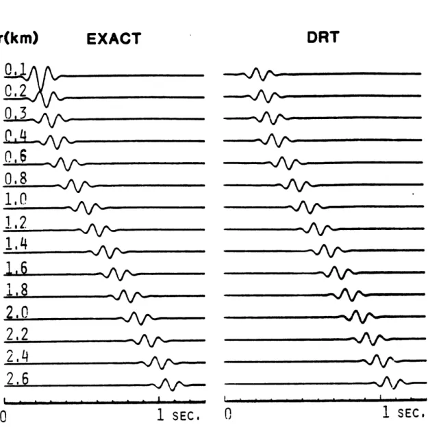
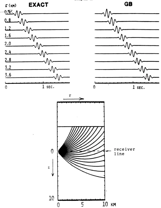
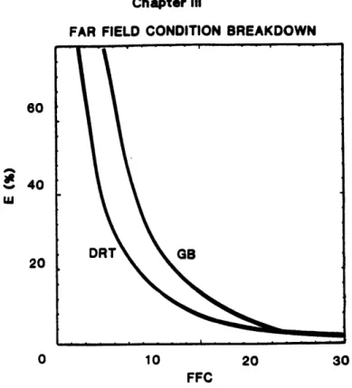
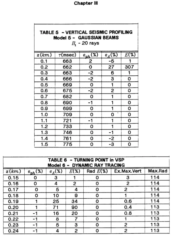
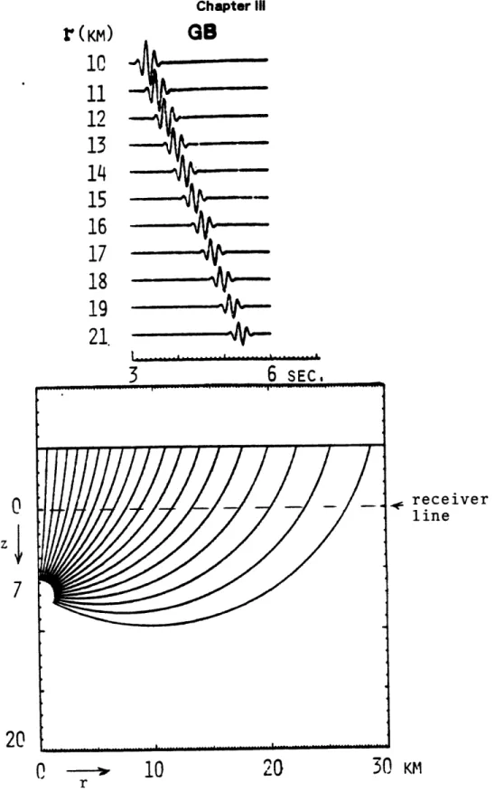
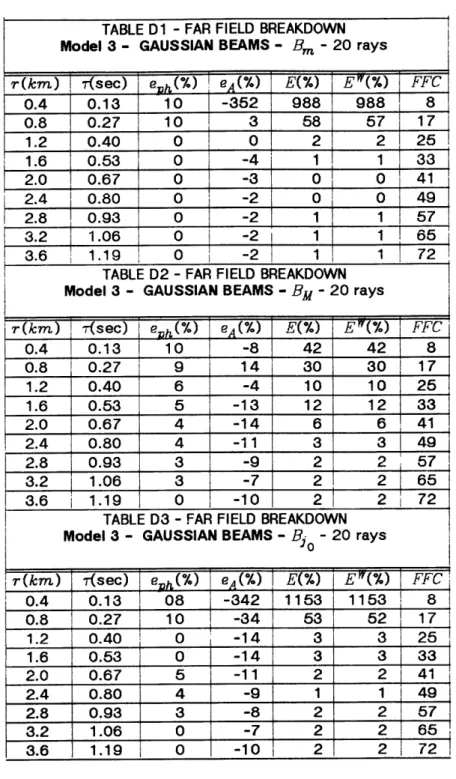
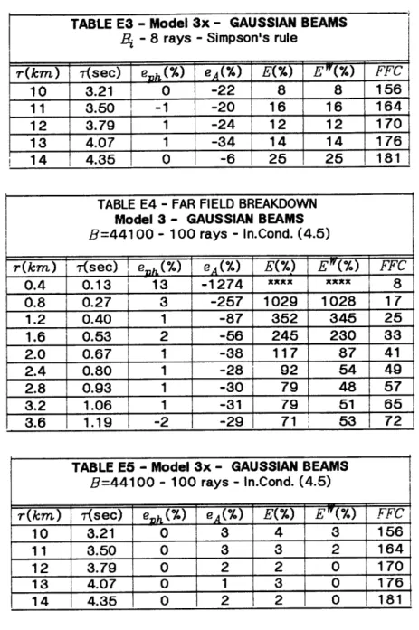
Chapter III deals with a canonical problem. The Green's function, in a constant gradient medium, is presented, for an explosive point source, in frequency and time domains. The analytical dynamic ray tracing (DRT) solution is re-derived with conditions stated in Chapter II. The Gaussian beam (GB) solution is investigated and new beam parameters are defined. Comparisons between exact and approximate solutions are made; for both methods, DRT and GB, conditions of validity are explicit and quantitative. An accuracy criterion is defined in the time domain, and measures a global relative error. The range of validity is expressed in the form of two inequalities for the dynamic ray tracing method and of five inequalities for the Gaussian beam method. Results remain accurate at ray turning points. For the type of medium considered, the breakdown of the dynamic ray tracing method is smoother and better behaved than that of Gaussian beams. As examples, a vertical seismic profiling configuration, and a shallow earthquake are modeled, using Gaussian beams.

Chapter IV describes the paraxial ray method, and its uses in modeling seismic waves. It is a flexible and fast method for computing asymptotic Green's functions. The method is an extension of the standard ray method, and a degenerate case of Gaussian beams. Accuracy is controllable, within ray and paraxial conditions. Comparison of results with finite difference and discrete wavenumber are very satisfactory. Examples for different heterogeneous media are shown.

A full-waveform inversion is then presented in Chapter V. A new approach, using tensor algebra formalism, is presented. Combined data sets (eg. VSP and surface

parameter. Data generated by finite difference is inverted and obtained estimates are accurate. VSP field data is inverted to estimate local geologic structure.

Thesis Advisor: M. Nafi Toksiz Title: Professor of Geophysics

-3-I am happy to acknowledge the help -3-I have received throughout the work of this thesis. My advisor, Nafi Toksiz, provided me with guidance and direction during all my stay at MIT. His skeptical eye and solid sense of geophysics have been of invaluable help.

I express my gratitude to Ari Ben-Menahem for providing me the opportunity to work with him during his stay at MIT. Chapters II and III of this thesis were done in

collaboration with him. His extensive experience in theoretical seismology and insights, along with his enthusiasm will always be remembered.

I have benefited from numerous discussions with Gilles Garcia. I learned about (exhaustive) quasi-Newton's methods for solving least squares problems, and hieroglyphs. He freely shared with me his stockpile of articles concerning the subject covered in Chapter V of this thesis.

I am grateful to Vernon Cormier and Roger Turpening, who have been a continual source of information and encouragement. I thank Greg Duckworth for reviewing the thesis and for his positive criticism, and Carol Blackway for spending her time acquainting me with the Burch data set, and providing me with information for the inversion of the field data. Interactions with Kei Aki, Michel Bouchon, Arthur Cheng, Raul Madariaga, Ted Madden, Ivan Pscencik, and Gene Simmons broadened my geophysical knowledge.

I am grateful to many of my colleagues over the years at MIT. To Tim Keho, for all the discussions, ranging from geopolitics to word decoding of WILD radio station songs, including science and sports. His humor and friendship are very appreciated. Numerous

Larrere, Frederic Mathieu, Michael Mellen, Bob Nowack, Fico Pardo-Casas, Benoit Paternoster, Michael Prange, Rob Stewart, Ken Tubman, Ru Shan Wu, Kiyoshi Yomogida, and many others, provided useful discussions.

Finally, I thank my parents, who encouraged me all the way through this long education, and for their altruistic guidance.

This work was supported by the M.I.T. Full Waveform Acoustic Logging and Vertical Seismic Profiling Consortia, the Compagnie Gdnerale de Gophysique, and the Air Force Office of Scientific Research.

Abstract ... ... 2

Acknowledgements ... ... 4

Chapter I. General Introduction ... 10

Nomenclature of Chapters Il-IV ... ... 1 5 Chapter II. 11.1 11.2 11.3 11.4 11.5 11.6 11.7 11.8 11.9 11.10 11.11 11.12 Chapter III. 111.1 111.2 111.3 Range of Validity of Ray and Beam Methods Introduction ... 19

Decoupling conditions for general inhomogeneous media...20

Hypereikonal ... ... 27

Ray series: eikonal and transport equations ... 37

Near and far fields ... ... 45

WKBJ approximations ... 48 Paraxial approximations ... ... ... 53 Gaussian beams ... ... 58 Conclusion ... ... 62 Appendix A ... 64 Appendix B ... ... 65 Appendix C ... ... 66 A Canonical Problem Introduction ... ... 69

Constant gradient model ... 70

Theoretical seismograms by DRT method ... .... 82

-7-111.4 111.5 111.6 111.7 111.8 111.9 111.10 Chapter IV. IV.1 IV.2 IV.3 IV.4 Chapter V. V.1 V.2 V.3 V.4 V.5 V.6 V.7 V.8 V.9 V. 1 0

Theoretical seismograms by GB method ... .... 88

Accuracy criteria ... ... 93

Model parameters and numerical details ... ... 95

Results and discussions ... 97

Conclusion ... 116

Appendix D ... 11 7 Appendix E ... 119

Modeling with the Paraxial Ray Method Introduction ... 1 24 Theory ... ... 127

Examples ... ... 1 35 Conclusion ... 1 53 Full Waveform Inversion Introduction ... 54

General derivation of the non-linear least-norm formulation ... 1...56

A priori information - Constraints ... 161

The linearized stochastic inverse ... 66

Data, parameter and model description ... 76

Examples ... 89

Conclusion ... 238

Appendix F ... ... 239

Appendix G ... 245

General Conclusion

Summary of Results ... ... 250

Suggestions for further research ... ... 251

References ... 253

Thesis Exam Committee ... ... ... 260

-9-Chapter VI.

VI. 1 VI.2

Symbolism, language, scientific formulae here are all synonymous.

- J. Bronowski

The notion of waves is one of the unifying concepts of modern physics. Their physical manifestation can be of very different nature (elastic, electromagnetic, quantum mechanic, gravitational), but their behavior remains describable mathematically, in common terms. The basic properties of waves is that they carry energy from point to point in a medium, and like moving matter, they have velocity and momentum.

Seismology deals with the generation and propagation of elastic waves in the earth. The data are seismograms, which is a measure of the disturbance caused by the wave during its passage through observers (seismographs) placed in contact with the earth. Typically these are records of particle displacement, or particle velocity, or particle acceleration, or pressure (in a fluid medium), as a function of time. The recorded seismic wavefield depends generally on three main mechanisms: (1) the wave generation (the source of energy), (2) the propagation through the complex media (scattering, diffraction, attenuation etc.), and (3) the seismograph measurement bias (quality of the coupling with the earth, partial information if it has less than three spatial components of recording, transfer function, etc.). These seismic records are very valuable if information regarding any of these three mechanisms is sought. Most importantly, they provide means of probing the earth interior. The advent of computers revolutionized seismology; data acquisition has improved enormously and sophisticated data processing is now possible. It is the second great tool, after analytical

mathematics, for theoretical developments.

Modeling

Modeling is a very useful approach in understanding seismic wave propagation in heterogeneous media and consequently helping the interpretation of data. For example, assume we have a specific earth structure in which we place sources and receivers. From the physical laws governing the behavior of seismic waves, one can determine, analytically or numerically, "synthetic" seismograms of the earth model. Modeling methods for complex media are numerous. There is no universal method that is applicable to all media. Each method is best suited for a given model, depending on the model's structure, source/receiver configuration, and the allocated computer time. Further, each method has its own assumptions and validity conditions that must be fully

understood before its practical use.

Hermann and Wang (1985), compare synthetics seismograms of several methods developed for plane-layered media, and list references of basic methods that deal with this problem. These are generally full-wave methods, in the sense that the full effects of the media are simulated and recorded. They are computationally expensive, and cannot be simply extended to handle more complicated geometries. Another set of full-wave methods, able to handle diffractions from sharp interfaces, concerns boundary integral methods. The media is limited to homogeneous layers separated by arbitrarily smooth interfaces, although extension for complex media can be made via asymptotic wave methods (see below). The methods treat each interface separately and with the continuity conditions at the interface, integral equations are set up for the wavefield. References for these methods can be found in Kennett and Harding (1985). Methods which consist in solving numerically the differential elastic wave equation in complex media, are called direct numerical methods. They are full-wave methods, and are

-expensive computationally. Finite difference (Alford et al, 1974; Kelly et al, 1976; Stephen, 1984) and finite elements (Marfurt, 1978) are the two main techniques.

The last set of methods is based on simple geometrical considerations. They are variations of ray theory, and will be called more generally, asymptotic (high frequency) wave methods. They are versatile, flexible and are generally used either directly in modeling, or indirectly in other methods requiring approximate Green's functions in heterogeneous media. These methods are not full-wave but are explicit, in the sense that individual wave types can be propagated separately. This offers the possibility of constructing progressively the full-wave character of the field. However if many wave types are sought, variations of these methods (Keller and Perozzi, 1983) must be considered.

Hybrid methods, combining advantages of compatible methods, are now under progress. Modeling real earth structures which would handle (1) multiples, diffraction and scattering effects, (2) critical region effects (caustics, shadow zones, etc.), and (3) interface waves (surface, head, etc.) is not an impossible task. Asymptotic wave methods are compatible with boundary integral methods, and can be an example of such a hybrid method.

The aim of this thesis is to establish, in some quantitative manner, the range of validity of asymptotic wave methods. Necessary conditions in obtaining Helmholtz wave equations from the elastodymanic wave equation are explicit. A hypereikonal is introduced that leads naturally to the ray solution for high frequencies. The focus is on dynamic ray tracing, Gaussian beam methods and, particularly on an intermediate method, called paraxial ray. We will not cover Maslov asymptotic theory (Chapman and Drummond, 1982), which can be obtained as a degenerate case of Gaussian Beams (Madariaga, 1984; Klimes, 1984). The paraxial ray method is shown to be a fast,

flexible and robust method. It is the method that we choose for modeling.

Inversion

The other fundamental task in seismology, is the extraction of medium or source parameters from data. Given a data set, estimating the parameters, require some assumptions on their prior values and constraints. Numerous approaches exist and, here again, each method has its own limitations. The three basic sets of methods are direct inversion, approximate direct inversion, and iterative inversion. They all yield, as end product, an image of the subsurface, and are sometimes referred to in general as inversion or imaging methods.

Direct inversion methods require the solution of an inverse operator such that when applied to observed data, it reconstructs medium properties exactly. These operators are difficult to obtain, particularly for more than one space dimension. Approximations, such as the Born approximation, simplify the problem and enable a direct solution to be found. A review of these methods with references can be found in

Esmersoy (1985). They generally assume the inhomogeneity to be included in a uniform background medium for which the Green's function is known exactly. However, extension to more complex background media can be done using asymptotic wave methods that provides approximate Green's functions.

Iterative inversion requires, generally, a forward model that is repeatedly used to generate synthetics. These synthetics are compared to data, and within a defined norm, the task is to minimize the norm of the data-synthetic discrepancy vector for medium parameters. Basic references on the subject are Beck and Arnold (1977), Luenberger (1973) and Aki and Richards (1980). Travel-time inversion has been, so far, widely used in seismology. But with the improvement in data acquisition systems, full-waveform

-13-inversion can now be attempted, since more information about the medium or source parameters is added. Examples of full-wave inversion for three dimensional (3D) medium parameters are found in Thomson (1983); for source parameters in Nabelek (1983); and for 1D medium parameters with vertical seismic profiling (VSP) in Stewart (1983).

The last chapter of this thesis deals with full-wave iterative inversion of combined VSP, surface reflection, multi-offset VSP or crosshole data. Forward model synthetics are generated by the paraxial ray method. The norm considered is the L2 or "energy" norm. The problem is presented within the framework of tensor algebra. The Gauss-Newton method is re-derived in this context. The heterogeneous media contains homogeneous layers separated by smooth interfaces. Sensitivity of the inversion to medium parameters is studied. Inversion of field data is presented.

Ao amplitude function of local plane wave

B parameter governing initial half-width of Gaussian beam

C constant factor calibrating ray methods to an exact solution co point source radiation pattern including source strength

c source strength, ratio co to source radiation pattern eA relative error of maximum amplitude of approximate signal

eph relative error of maximum amplitude time of approximate signal e1 relative error of travel time of approximate signal

E relative power error of approximate signal on the entire trace

EW E on wavelet time window

F0 c1/pl/ 2, strength of point source (dimensionless)

f general source radiation pattern including source strength FFC far field amplitude condition

FRN1 Fresnel 1-condition

FRN2 Fresnel 2-condition

Ia P wave coupling vector

G(W f0o) scalar Green's function

Gr radial Green's function in (r,z)

Gz vertical Green's function in (r,z) HFC high frequency condition

h 7- 1, vertical distance between a(O) and a=O

I unit dyadic (tensor)

J Jacobian of cartesian to ray coordinates

-JS surficial Jacobian of cartesian to ray coordinates jo ray parameter, takeoff angle, bi-spherical coordinate

j ray angle of incidence

K Gaussian wavefront curvature

KR R- 1, local ray curvature

Kw acP/ Q=i 1, total curvature of wavefront (or phase front)

SaP/

k &/ cx, P wavenumber

0 al/ wo, medium's characteristic length L local half-width of Gaussian beam

mO source seismic moment

M receiver / observer location

Mo point source location

NHI non-horizontal incidence of ray condition

n cartesian coordinate perpendicular to the ray p sinj/ a, ray horizontal slowness, ray parameter

-P4, unit vector tangent to the ray P a- 1 dQ/ ds, functional in the eikonal

PRX paraxial ray condition

Q functional in the eikonal

r radial distance from vertical z axis

rt (zo+h)cotjo, radial coordinate of turning point of ray

RCC regularity of ray-centered coordinate system condition

R local ray radius of curvature Rw local wavefront radius of curvature s arclength along a specified ray

S hypereikonal

t time

T generalized travel time

Uparticle displacement vector in time or in frequency ZU Green's function along t in (4,z)

us Green's function along z in (,z)

v P or S intrinsic velocity of medium

VF Fresnel volume

W P wave vertical displacement in (r,z) coordinate system W11 W computed by the Gaussian beam method

Wr W computed by the dynamic ray tracing method

z vertical axis

Zt R-h, depth of turning point of ray

a compressional (P) wave velocity of the medium o P wave velocity at the source location

B shear (S) wave velocity of the medium

Sa2/

p2

71,2 ray parameters

A source-receiver distance in a homogeneous medium

E cumulative error along the ray

Ea P wave coupling scalar

A wavelength

X First Lame elastic parameter

/, Second Lame elastic parameter, shear modulus

-7/ to, bi-spherical coordinate, curvilinear coordinate along a ray Sunit vector tangent to the ray

-17-p density of the medium

Po density of the medium at the source location

Pi,2 principal radii of wavefront curvature a point source time function

point source spectrum

7 source - receiver travel time

weight function for the Gaussian beam

pd P wave potential

P2 S wave potential

Helmholtz potential aCpar Parabolic potential

W angular frequency

Wo medium's threshold frequency

Nature is not a gigantic formalizable system. In order to formalize it, 'we have to make some assumptions which cut out some parts.

We then lose the total connectivity.

- J. Bronowski

1. INTRODUCTION

Asymptotic wave theory is subjected to a number of fundamental restrictions which put severe limitations on its applicability, These restrictions involve three types of physical parameters: frequency, distance and gradients of structural elements. The conditions are formulated in the form of inequalities. If any of these inequalities is violated, ray theory becomes (progressively or rapidly) invalid and we must resort to the full-wave theory or other valid approximations. The limitations of ray theory fall into several categories, each arising in connection with a different type of asymptotic approximation. Each category renders its own conditions for the validity of seismic ray theory.

There exist today a few basic ray-methods which are interrelated. The oldest is the eikonal method (e.g., Born and Wolf, 1964; Luneburg, 1964) upon which the entire field of geometrical optics is based. It became a very useful tool in studies of seismic wave propagation (e.g., Singh and Ben-Menahem, 1969, Cerveny et al., 1977; Aki and Richards, 1980; Cerveny and Hron, 1980) Next came the WKBJ and the saddle-point approximations at high frequencies (e.g., Bremmer, 1951) with some new development

-19-and variants (e.g., Kravtsov, 1968, -19-and Kravtsov -19-and Feizulin, 1969, Chapman, 1978). In recent years, the advent of computers allowed seismologists to look for fast and efficient algorithms to calculate collimated wave fields in inhomogeneous media. The paraxial wave approximation, especially in a ray-centered coordinate system was found to offer some advantages (e.g., Landers and Claerbout, 1972; Corones, 1975; McDaniel, 1975; Palmer, 1976, 1979; DeSanto, 1977; McCoy, 1977; Bastiaans, 1979; Cerveny et al., 1982; and Haus, 1983)

In addition, certain efforts were made to harness the Kirchhoff-Helmholtz integral (e.g., Baker and Copson, 1939) to the evaluation of seismic fields (e.g. Kravtsov and Feizulin, 1969; Scott and Helmberger, 1983; and Carter and Frazer, 1984) There is now a growing need, both in earthquake seismology and in seismic exploration, for computational methods that can render sufficiently accurate solutions to wave propagation problems in three dimensions. In this chapter we shall examine the validity of the various approximations involved in the asymptotic wave theory.

2. DECOUPLING CONDITION FOR GENERAL INHOMOGENEOUS MEDIA

The elastodynamic vector equation for isotropic media, in the absence of body forces, can be put in the compact form

p-0 = V[(X + 2)V 0] - Vx(LVx () + 2V/4*Vx(I x ), (2.1)

at2

where I is the unit dyadic, U denotes the particle displacement vector at point M(r')

and time t,p is the density, and X and A are the Lame elastic parameters of the medium.

1

1

Vx(I

x

-IxVx U -IV*U+

-(VU + UV).

2 2

Introducing the notation

pa2 = X + 2/, _pf2 _{= A,} and applying the vector identities

V(~4) = 1P VP + cp V4',

V.(pA) = p V A + (Vp).A ,

Vx(qB) = q Vx B + (Vq) x -,

we may recast Eq (2.1) in the form

2 = 2 V ) - VX ( 2 VX ) + P (2 V. )

-at2 P

YJIx

(# 2x

+ 2#12 Y + Vx ( x 0)

Taking the divergence of Eq. (2.4), applying to it the Fourier transform over t and defining N = a2 V ,

A

=

Vx U,

,

Jp =

P

it is possible to transform Eq. (2.4) into

V2N + Jp VN + k2N = (2# + p). Vx A - t,

where

=NVV*. p -A *Vx p + V 2#2(g fp)l :Vx(I X ') + 2.p- * xAi

(2.8)

(2.9)

The advantage of writing Eq (2.1) in the form (2.8) is obvious: It separates the terms of

- 21

-(2.2)

(2.3)

(2.4)

the equation into three distinct groups according to the order of the derivatives of the constitutive parameters p and

P.

(2 p + *p) -Vx A. Further change of variable

b = p /2N, = 1/2A,

followed by neglection of terms of the order (1p)2, leads us to the scalar wave equation

V2b + k b = (2p + p). Vx + O(E2&; 2); ), (2.10) where

Ea = a C s = ; p = p"" (2.11)

Similarly, by taking the curl of Eq(2.4), we obtain to first order in Ja, g# and gp

V2A + (p - j). VA - x VxA + kA=

=

[

v

_A

_{- vB gP}

=

=

'2J[g

+ 2

-J]xVb

;i

p;

(2.13)

Note that since (2.1) does not have an ezplicit dependence on VX, as it does on V/D the gradient of the compressional velocity a does not enter explicitly into Eqs. (2.4) -(2.12). It is, however, implicit via Eq.(2.5) and the gradients of N and b in Eqs. (2.8), (2.10) and (2.12). For that reason we must require, as we indeed do in Eq. (2.14) and (2.18), that ea << 1.

1. Smooth inhomogeneous media: second order terms in the coupling vectors are neglected but first terms are kept. The equations of motion are coupled [Eq. (2.10), (2.13)].

2. Weak inhomogeneous media: first and second order terms in the coupling vectors are dropped. The equations of motion are totally decoupled .

Eqs. (2.10) and (2.13) are the first order elastodynamic equations for the coupled shear and compressional wave motion in general inhomogeneous isotropic media. The entities jp, fa and '# are the P-SV coupling vectors. Landers and Claerbout

(1972) and Landers (1974) numerically integrated equations similar to our (2.10) and (2.13) in two dimensions to recover the seismic wavefield. In the context of ray-theory we assume a total decoupling of P-SV motion. A necessary condition is

Ea << 1, &E <<1, Ep << 1 . (2.1 4) In media that obey (2.14), the material properties change slowly over distances of order of a wavelength. The corresponding equations of motion in such media will then simplify to

V2b +k b = 0, V2 + k2B = 0. (2.15a) Thus, for weak inhomogeneous media, the functions

b =pl/2a2V.U and B =p1/2 2Vx U, (2.15b) obey the respective scalar and vector Helmholtz equations. In earthquake and exploration seismology, there are many instances where this approximation is sufficient. If first order coupling terms of P and SV waves are retained, then one must solve Eqs. (2.10) and (2.12) simultaneously. In either case, the spectral displacement field

U(M,) is recovered by further integration and differentiation,

-4rU(9) = - f d + x Vx 0 ) d3, (2.16)

If -1I 1 - 11

where V is the del operating on the ? coordinates of the integrand. The decoupling conditions (2.14) can also be written in the alternative form (A = wave length, k 2 = wave number, and k = for P waves and k = for S waves)

A a

A << min Vp -~- or k_a o10 >> 1 , (2.17) or

<< << 1 << 1 (2.18)

where 10 is a characteristic length at a given location, and may vary from point to point in the medium. Condition (2.18) refers to a local property of the elastic medium. It can be shown in a vertically or radially varying medium that is radius of curvature at

the lowest point of the ray (turning point).

The mode decoupling condition that we shall use is

W >> wo,

max

Il

Va , VP

,a

(2.19)

This condition defines a virtual threshold frequency which must be surpassed by the wave frequency w. Note that the threshold frequency wo is tied to the characteristic length lo via the relation lo1o = a . We shall show later that (2.19) is physically more meaningful than (2.18) in the sense that w0 exists even when exact decoupling renders (2.18) meaningless.

Note that in homogeneous media with material discontinuities, l0 assumes the geometrical meaning of radius of curvature of the discontinuity. If, for example, we

consider compressional wave propagation in a sphere of radius a, (2.17) will be replaced by

kaa >> 1 , (2.20)

which means that the wavelength must be much smaller than the sphere's radius. Note that this condition does not mean that, at the interface, P and S wave are not coupled by boundary conditions, but that their propagation, away from the interface, remains uncoupled (independent Helmholtz equations for P and S waves).

The inequalities (2.14), (2.17) and (2.18) are only necessary conditions for the elastodynamic equations to yield approximate decoupling of P and SV waves. The following note is appropriate in this connection: The smallness of sa, E# and ep does not

imply that Va V and cease to play a role in shaping the amplitudes of

I ' #

P

seismic waves in the earth. On the contrary, these entities turn out to be essential in the seismic theory of Gaussian beams and dynamic ray tracing. Indeed, if we solve the Helmholtz equations (such as Eqs. (2.15a) in coordinate systems where the metric scale factors depend on the velocities a and # (such as the ray-centered coordinate system or the intrinsic coordinate system)), second-order derivatives of a and P reappear in the Helmholtz equation.

In weakly inhomogeneous media we assume a decomposition of the displacement field analogous to the decomposition in the case where the medium parameters depend on a single coordinate (see for example Ben-Menahem and Singh, p.417, 1981)

=

2

Vx (

2

3) , (2.21)

where & is a (unit) vector subjected to certain restrictions, and the potentials Oi obey the respective Helmholtz equations (V2 + k?)P = 0 i = 1, 2. The condition under which

-(2.21) holds is that of Eq. (2.19) in vector separable coordinate systems. Substitution of Eq. (2.21) into Eqs.(2.15) links the potential systems (b, A) and (P1, 1 2, s3). The relations are b = -w2 01 and B = - 2VX(a312) + #VX VX (8P3).

Vertically Inhonogeneous Media

In the special case where the inhomogeneity of the elastic medium depends on one cartesian coordinate z, the analysis becomes simpler and mathematical tools are available to solve the equations of motion. Three important results can then be derived:

1. Exact decoupling of the P and SV wave motions is possible only in special cases where the constitutive parameters satisfy a pair of nonlinear ordinary differential equations (Hook, 1961, 1962; Alverson et al., 1963; Lock, 1963). We shall deal with an example of this category in chapter III.

2. Under less restrictive conditions (keeping first order terms in Ea , e, and p) the field can still be represented by an expression similar to (2.21)

1 1

= V(f 1) -

-VxVx

Substituting this expression in Eqs. (2.8) and (2.13) and keeping terms up to first order derivatives in X, p, and p, a straightforward, though lengthy, analysis yields two coupled equations for the potentials 01 and CP2

V2p + k 1 1 1 12 V2

-

p

az

V2 2+ + k2 P2 = 21 1(2.24)

p az

211 A X + 2__, (2.25)

are scalar coupling factors, and primes indicate derivatives with respect to z. A perturbation scheme for the solution of (2.23) and (2.24) is presented in Appendix A.

Lock (1 963) derived an exact solution of the elastodynamic vector equation for

p(z) = /(O)ez; X(z) = X(0)eaz; p(z) = p(O)e . (2.26)

In this case a = - = 0, gp = aez = const. and Eq. (2.4) reduces exactly to our Eqs.

(2.23) to (2.24) with p'/p = a, 7712 = "7-1, 9 21 = a(2 - y), 7 = (X + 2pu)/ u. Since the velocities have fixed values, the rays are straight lines and the coupling is effected through the constant density gradient alone.

From this point on we shall assume a total P/S decoupling. Hence, we do not have to deal any more with the elastodynamic vector equation itself, but rather focus our attention on approximate solutions of the scalar Helmholtz equation.

3. HYPEREIKONAL

Let us now examine the Helmholtz equation for general inhomogeneous media. A convenient mathematical vehicle is afforded by a general orthogonal coordinate system where the only constraint is that one of its coordinates is the wave travel time -r. This

system will be denoted (7, ,Y72), with corresponding scale factors h. h1 and h2. The

2

scalar Helmholtz equation V2ip + = 0 in this system is

___+1 h-2 h- 2

+h

h r h2 tT hr 1 h 1 h2 d2 202

We take to be of the form = A0( ,y,112 ;0)S(-r;w). and substitute into (3.1). After

-some intermediate steps, (3.1) reduces to

2

2S 2 2 2Ao v2 S V2, + 2 * VT =0. (3.2)

h2 Sd 2 + Ao S dT Ao

Assume that the terms involving first derivatives with respect to T are of different order than the rest. This yields the two equations

v2 12S 2 V2Ao V2 2S + W2 + v 2 0, (3.3) h2 Sd72 Ao and VAo V2T + 2 VT = 0. (3.4) Ao

Consider the class of inhomogeneous media such that

2

V2 A o + ~ o = 0 , (3.5)

where oc and v2/h 2 are either constants or a slowly varying functions of the coordinates. In cases where both are constants, an exact solution of Eq. (3.3) is

h

-iwr T (1 - 2/ u2)1/2 (3.6)

S(-;w) = e V G

The S functional in (3.6) is defined as the hypereikonal. Equation (3.4) is the

transport equation with an exact solution

h 1/2

Ao(r,y1,, 2;) = f (71,72;w) hi (3.7)

where f(y,y 2;o) is a function independent of T. This solution assumes h1 h2 0. In the case where 71 and Y2 are the two spherical angles, f can be interpreted as the product of the radiation pattern of a source located at the origin of the spherical coordinate system times the source strength. Thus, for example f(Y1,7₂;w) = CO

(constant) the source is a point explosion. Let J be the Jacobian of the transformation from cartesian to the general orthogonal coordinate system (7r,7,2).

J _ D(x,y,z) h-rkh2 (3.78)

D(,7Y1, 2) - h.(h.h₂. (3.7a)

Define the surficial Jacobian as JS = J/h - hlh2. Equation (3.7) then reads

Ao = f il/ 2 (3.7b)

JS is sometimes called the spreading function.

The solution of the Helmholtz equation can then be written in the compact form h

h '1/ jw (1 - 2/ 2)1 /2

A0 S

= f

For wc = O0, or w >> .c, this solution reduces to the ray solution (see section 4) or the WKBJ solution of the wave equation (see section 6), respectively. In media where (3.8) holds, there exist a cut-off frequency c; below which wave propagation is not possible. The medium cut-off frequency, defined as, c = v(V2Ao/Ao)1 / 2, may be complex. Media for which oc is complex will not be treated here and a special investigation will follow in a sequel paper. The factor (1 -w2/ W2)1/2 in equation (3.8) indicates the presence of a second order effect of dispersion which is usually neglected for seismic body waves at high frequencies.

The hypereikonal formulation for the Helmholtz equation can be extended in a straightforward way to the vector elastodynamic wave equation (2.1). In Appendix B, we show how this can be achieved for the special case of vertically inhomogeneous

media.

-Vertically Inhomogeneous media

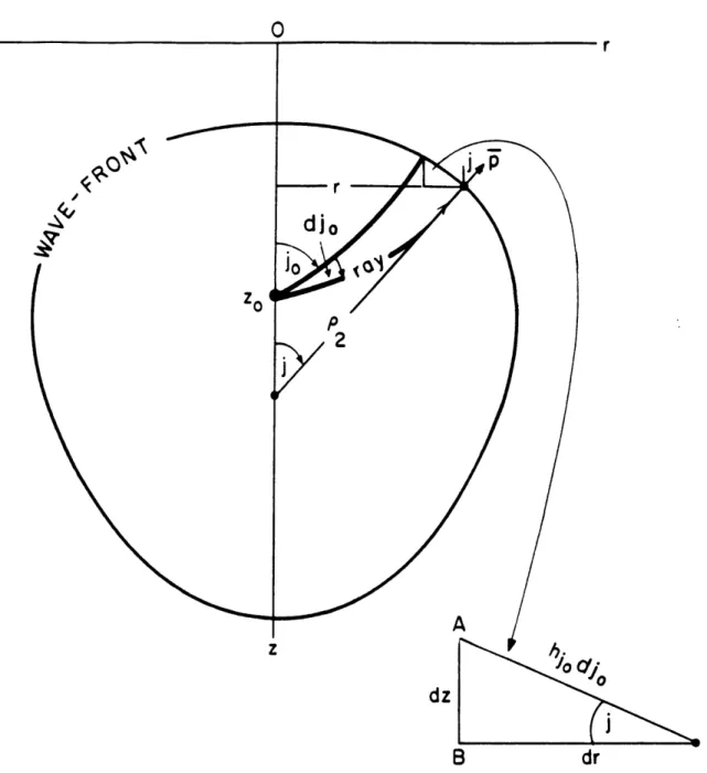
As an application we shall derive in closed form the results given above in the case where the medium's properties are only allowed to vary along the z direction. A convenient coordinate system is the intrinsic coordinate system (Yosiyama, 1940). In a vertically inhomogeneous medium, we define a cartesian coordinate system centered at 0 (figure 1). The cylindrical coordinates of a general point M are (r, a3, z). A seismic source is placed on the z axis at M0(O,0,zo). We define new coordinates M(i-,j 0,d) relative the origin Mo, where 1 is the azimuth angle of the cylindrical system. The transformation-equations linking the coordinates (z,r) and (-,j 0) are given by the implicit integral relations

Z z

r

=

z0 z₀

where

g v()' P = g(zo)sinjo (3.10)

These are the standard travel time equation, T, and horizontal slowness, p, in Herglotz-Wiechert formulas (Aki and Richards, 1980); jo is the takeoff angle. It is understood that p is held fixed (z independent) during the integrations. Thus, although jo is indeed a coordinate, it acts as a fixed parameter during the intergration. v denotes either a or

p.

For any given velocity distribution v(z), Eq. (3.9) defines the relations

r = r(z,p) and 7 = r(z,p). For any given values of z and r, these two relations define the pair (T,j 0) and vice versa. For a fixed value of p (i.e., jo), the r integral in (3.9) defines a curve r = r(z) in the plane 1 = const, and the T integral defines the travel time along this curve from zo to z.

Mo (So)

jo

(T,j,e

₀

)

er

r

Figure 1. The intrinsic coordinate system

31

-"- - - - I- -.

The angle j between the vertical and the tangent at any point on this curve is obtained readily by differentiating r with respect to z for fixed p. This is the ray angle of incidence.

bJ

Solving for p and comparing with (3.10) we find

S= sinj sinjo (3.12)

v(z) vo

where vo = v(zo). Eq. (3.10) is the ray equation and Eq. (3.12) is Snell's law. For a fixed value of jo, the ray equation is given by a relation r = r(z;jo) . With these definitions, one can verify in a straightforward manner the following statements:

A. The line element of the new system is

CI2 -h2dT 2 +hd d 2 _.hdj

(3.13)

where the explicit expressions for the scale factors are:

3

h, = v(z); h = r; hio p (g -P 2)1/ 2 cOtj0 2 (g2 _p

2

) 2 dz . (3.14)

g z_o

Hence, the coordinate system (T,jo,) is orthogonal.

B. The wavefront equation is obtained by eliminating p between the relations

z z

T₀ =f 92(g2 _p 2)-1/ 2dz and r = fp(g 2 -p2)- 11/2dz. At any given time - =To0

zO _zO

the wavefront is a surface of revolution generated by the plane curve (figure 2)

r

04

djo

zo

o

P

₂

Figure 2. Cross-section of wavefront at 15 = const .

-

33

-A

Since on this surface d-r = 0, we have from Eq. (3.13) and from the geometry of a line element on a general surface of revolution

d 2 h. 29 2 h 2 = r2d 2 + 11

dr

Therefore, on the wave front, up to a sign

dz 1 dr 1 dz

= tanj; ho = COS - sinj do (3.16)

The geometric interpretation of Eq. (3.16) is evident from figure 2. An alternative interpretation of hjo is obtained when we differentiate r in Eq. (3.9) with respect to jo

at fixed z and use Eq. (3.14)

h cosi[ I (3.17)

C. The Gaussian curvature of a surface of revolution is defined as K = (p1P2)-1 where p, and P2 are the wavefront principal radii of curvature (eg., Eisenhart,

1909). In our present case

dz 2 dr dsinj _(3.18) P d22 z dr dr2 _

(dz121/2

Pdz2

+

sinj

K = dr dr2 _ sin dsin = sinjcosj j (r) (3.19)

l

dz2l r dr r dr

D. The divergence coefficient (e.g., Ben-Menahem and Singh, 1981) is given by

SvoPo

rio

11/2

the expressionX= rcos j ,where lul = Xe " I uol , u being the particle displacement. In terms of the scale factors and with the aid of Eqs. (3.7) and (3.17), it is found that

x=Po

o

Ao

sino)1/2

[

h,2

1/2

X = , Ao - c1 ( ) (3.19a)

p v c1 vo hhjo

The point source constant introduced earlier, co, is here equal to c (sinjo/vo)1/ 2 ,

where c1 is the source strength. Using Eq. (3.12), we can'also write

X = (p2hi )-1/2 (3.20)

If we substitute for sinj in (3.16) from Snell's law (3.12), and evaluate thed

dr

derivative at the wavefront, we obtain

cotj _

COtjo

1

o - + =-, (3.21)

where R = is the radius of curvature of the ray at the wavefront. In

homogeneous media p, = hjo. In weak inhomogeneous media we have approximately

tanj_o

p i ta-- hj (3.22)

The Jacobian of the transformation from cartesian to intrinsic coordinates is

J = D(x,y,z)/ D(T,jo,3) = h ohjo (3.17a). If we consider a homogeneous unit focal sphere around the source, Eq. (3.14) will render for this sphere (h) 0 = vo, (hO)o = 1, (hjo) = sinjo. Denoting the Jacobian on the focal sphere, Jo = vosinj0, we find from (3.1 9a)

-X

Po Jo ; Ao = cv (3.23)

x

=

;AO= l

oJ

--Note that in weak vertically inhomogeneous media, the total curvature (Eisenhart,

1909) of the wavefronts is

I 1/ 2 Ao

K. = (pP2)-1/ 2 _tanjo tanj 0 (3.24)_.C)

We thus see that Ao is a fundamental quantity that is linked to divergence coefficient, the Jacobian and proportional to the total curvature of the wavefront. In cases where (tanj / tanj 0) /2 is close to unity, Ao is close to the total wavefront curvature.

A class of media for which Eq. (3.2) holds is found in the following way: we put

r

rh

Ao = c D = i, j ' (3.25)

v D9 sinjo

where D is a certain distance. It then follows that Eq. (3.5) assumes the new form

v2 vD--2 -I 1 d2 v dv 2 (3.26)

Ao D

4dz

In a homogeneous medium D V2 0, v' =v" =0 and wc = 0 wo. In a medium with a constant velocity gradient v = v(0)(1 + T7z), one proves that

v2 DV2 1 v D dv 0. Eq. (3.26) then yields the exact result D D Oz dz

_ 1 l V (0) Wo • (3.27)

c 2 dz 2

In a medium with a linear gradient v = v(O) (1 + 7l z + 72z 2)

v2 2A 1 2(0)[ -472] +

O

So, at least in the far field, the cut-off frequency is at

V (O) (2 _ 42)1/2. _(3.29)

However wo = (0) (71 + 2z72). This includes Eq. (3.27) as a special case wherever

772 = 0.

The threshold frequency, co, characterizes the heterogeneous medium. In order for asymptotic wave methods to be applicable in such a medium, the wave angular frequency ,co, must be greater than oo. This is the mode decoupling condition derived in section 2, and expressed in (2.19). Another medium characteristic frequency is the cutt-off frequency, c, introduced in (3.8). The wave frequency must be greater than

oc so that second order effect of dispersion can be neglected.

We thus see that in media where the velocity profile can be represented by a polynomial of degree one, co = wc. In general, oc and wo depend upon the coordinates, and their equality is not obvious. In the special case of the paraxial approximation (and ray theory) their equality is postulated on the basis of dimensional analysis.

4. RAY-SERIES: EIKONAL AND TRANSPORT EQUATIONS

Geometrical optics is based on the first term of the asymptotic-series solution of the Helmholtz equation

I(M,o) = eirr(M) (4.1)

n =o

The substitution of

O(M,w) = Ao(M) eic 'r(M), (4.2)

into the Helmholtz wave equation [sometimes known as the ansatz of Sornmerfeld and zrunge (Cornbleet, 1973)] leads to

-+ + - + i 7 + 2 * V= 0. (4.3)

If Ao is a sufficiently slowly varying function of the coordinates over a wavelength scale, we have

S>> c. (4.4)

This is defined as the high frequency condition. Then, equating real and imaginary parts on both sides of Eq. (4.3) we obtain the well-known eikonal and transport

equations respectively

(V7 2 = ; (4.5)

VAo

V2T + 2 V * VT = 0. (4.6)

Ao

The characteristic equations of the eikonal (4.5) yield rays 0. The solution of the eikonal has the physical meaning of the travel time along a ray 0 connecting the source

Mo(s o) to a receiver at M(s), where s is the arclength along the ray measured from a given fiducial point. It is given explicitly by the equation

(s)

=

The transport equation (4.6) involves the travel time i(s) and a function Ao(s) with the physical meaning of an amplitude of a local plane wave along the ray coordinate s. It is the same as that derived in the previous section (3.4). The surface 7(s) = const. yields the wavefront (or phase front). The solution of the transport equation is given explicitly in (3.7).

W2 in (4.3). The transport equation is of lower order in frequency, since it is obtained by equating to zero the coefficient of w. For high frequencies the remaining term in (4.3) is assumed of order one (high frequency approximation).

Having defined the concept of a ray, the coordinate system introduced and used in the previous section remains valid for characterizing rays. The coordinate system

(,71',2) introduced in the beginning of section 3, will henceforth be called ray

coordinates. A special case is the intrinsic coordinate system (7,j 0o,,), which will be used in the present context.

However, it is convenient to solve the eikonal equation in the ray-centered coordinate system (s,ql,q2). The process of solving the eikonal equation in this

orthogonal system is known as dynamic ray tracing. s measures the arclength along the ray 0 from an arbitrary reference point to the receiver position M(s) and ql,q2 are

the cartesian coordinates in the plane perpendicular to 0, with origin at 0. Details of this system and its regularity are described in Cerveny (1983a). The scale factors of this coordinate system with respect to the cartesian reference frame are

1 6v 1 h1

h = +q 1 + q2 -- ;L hLq 1 = hq2

-hv = +q l 2 q

The partial derivatives are evaluated at q, =0.

Defining Kw as the local wavefront (or phase front) curvature matrix (in the vicinity of 0), the eikonal equation in the ray centered coordinate system of 0 is written in the form of an ordinary non-linear differential equation of the first order of the Ricatti type for I~, which cannot be generally solved by analytical techniques. Letting

K(s) v(s) P(s) Q-1 (s), the eikonal is expressed as a coupled first-order ordinary linear differential system (Cerveny, 19 8 3Q)

-dQ(s) _ v(s) P(s), _(4.8)

ds

dP(s) - -(s) - 2

V(s) Q(s),

ds

where v is the P or S wave velocity and V -

=

with specified initial conditions (point source or line source), for the 2 x 2 matrices

P(s) and Q(s) determines K(s). K.(s) is symmetrical, and in 2-D media, it reduces to the scalar Kw (total wavefront curvature).

It is shown that in ray centered coordinates, for a given point s on 0, the transport equations for the P wave principal component ,a (along the tangent vector to 0 ) and for S wave principal components IL0 (along 1 ) and 1iZ2 (along C2 ) are

independent. The ray centered coordinates "untwists" the ray of its torsion, at every point s of 0, to its initial value at Mo. The unit vectors that constitute this coordinate system are sometimes called the polarization vectors. In a weak heterogeneous medium, the analytical solution of the transport equation for a receiver M(s) is given by

Ao(s) = co VS ) , (4.9)

where co is a constant characterizing an explosion source. For other sources embedded in a homogeneous focal sphere, co must be replaced by f ( 1,72;w), as defined in equation (3.7). This is nothing else than (3.7b) expressed on the ray 0. For P waves,

Ao- I ,I1 and v(s) = a(s) , and for S waves A0 =I ' , or Ao

Ii#2

21,

v(s) = f(s). JS is the surficial Jacobian of the transformation from cartesian to ray coordinates (T,71,' 2)- It is computed via JS(s) = det[Q(s)], and measures the cross

sectional area of an elementary ray tube surrounding Q . jS is related to J with the identity given above (3.7b). Here h,=vhs . On the ray we have h, v. The Jacobian

JS = h 1 D(z,y,z)

i D(,7Y,7 2) h

1 _D(z,y,z) D(7,ql,q2)

S D((7,ql,q2) D(Tr,Y1, 2) or in terms of scale factors

JS - 71h72 =h lhq2 det[Q] = det[Q]. (4.9a)

Q can be viewed as the Jacobian matrix of the transformation from ray centered to ray coordinates, and consequently det[Q] is the Jacobian of this transformation.

The displacement is recovered via (2.21). Recalling that Ao and 7 are only functions of s, and that in the case of P waves the displacement is along the ray

p,

have

U

Since the ray solution is the far field contribution of U, (condition (5.9)) we have for the ray solution

Or = CO (PV jS)-1/2 i Z' . (4.11)

Expressed in terms of a divergence coefficient (3.23) we have

Ip

S

1/2

=

p v is

W eir

p,

where C-= / iw = cl/ (p -1/ 2 vo). Parameters with subscript 0 denote their value at the homogeneous unit focal sphere surrounding the source. For a point source Jo=sinjo

(see 3.23).

Oumulative Error

So far we have not raised the question of the error produced by replacing the

-exact solution of the Helmholtz equation by the first term in the geometrical optics approximation. Let then

S3= [

+ E =

o

j'

where 0w2/w( 2)1/2

where - = Aoe as derived in equation (3.8), q = Aoe 'Gr , and a is the

correction term.

With the provision c >> wc we have from (4.13)

22w

Therefore, in order to have small relative error we must have

>> o 27. (4.15)

This condition is defined as the Fresnel 1-condition. It is re-derived, within the paraxial approximation in section 7, for a homogeneous medium.

Note that

lim = 0. (4.16)

This means that in the radiation zone of inhomogeneous media (i.e. when eq. (4.4) is satisfied), the error due to ray theory tends to decrease with the increase of the frequency.

We can view (4.14) as a cumulative error along the ray and condition (4.15) ensures that this error stays small. This can be shown by substituting (4.13) into the Helmholtz equation and using the transport equation (4.4). We find that e obeys its own Helmholtz equation with a forcing term

2 V2AO

V2,C+ - -o . (4.17)

v2 Ao

Direct integration of Eq. (4.17) renders

1 V2Ao (418

7

f A-P o G( I o) o , (4.18)

where the Green's function G satisfies

2

v2

c

In order to estimate the integral in (4.18) we apply the mean value theorem over a finite volume element which is assumed to be the Fresnel volume. As we shall see in section 7, this volume is a paraboloid of revolution. The source-receiver distance will be taken to be U7. The volume is then

= T r2 U7, (4.20)

where U is the average velocity along the ray, ro =A v T is the first Fresnel zone radius at the observer.

Eq (4.18) then becomes

1 V2 A0

S ---- o G VF. (4.21)

45r Ao

aveTrage

with Fresnel volume, VF, given by (4.20).

However, the absolute value of G is approximately equal to the wavefront curvature, RE1, which is of same order as (UT) - 1 , and V2Ao/Ao = 10-2. Substituting these values into (4.21) we find that the relative error e/io is small, if (4.15) is satisfied (within a factor -). The relative error can thus be seen as a cumulative error

2

-along the ray.

Even within the limits of the above restrictions, the ray-series will fail to represent the solution of the Helmholtz equation at critical points where the Jacobian in (4.9) vanishes. For a vertically heterogeneous medium, according to Eq. (3.20), this failure can be avoided if (see figure 2)

h5- X 0 P2 r 0 (4.22)

5. NEAR AND FAR FIELDS

We shall first derive intuitive conditions for inhomogeneous media from extrapolation of the homogeneous case. Then, we shall define formally the far field condition directly from the eikonal and transport equations. In a homogeneous elastic medium, the displacement field of seismic point source such as an explosion is given explicitly by the expression (e.g. Ben-Menahem and Singh, 1981)

- vpa _(5.1)

4rrp

_,

4-p 02 a A &

where mno is the source seismic moment, ka = w/ a is the compressional wavenumber, A is the source-receiver distance and 6A is a unit vector along A.

If kaA >> 1 or A >> A, or T >> wave period, the expression

-* O-imok I

kl

47T(X + 2A) A

I

represents the far-displacement field. Since kaA = WA/ a = 07 where T is the P-wave travel-time along the ray, it is expected that the far field condition in inhomogeneous media will read accordingly

S>> to , (5.3)

where r given by (4.7) is the travel-time along the ray with intrinsic velocity v(s) (v denotes either a shear velocity P or a compressional velocity a) and to is some

threshold time which is characteristic of the particular inhomogeneous medium under consideration. This threshold-time must be related to the threshold frequency of Eq. (2.19) through the relation