Imperfect supercritical bifurcation in a three-dimensional turbulent wake

HAL Id: hal-01164472

https://hal-ensta-paris.archives-ouvertes.fr//hal-01164472

Submitted on 17 Jun 2015

HAL is a multi-disciplinary open access

archive for the deposit and dissemination of

sci-entific research documents, whether they are

pub-lished or not. The documents may come from

teaching and research institutions in France or

abroad, or from public or private research centers.

L’archive ouverte pluridisciplinaire HAL, est

destinée au dépôt et à la diffusion de documents

scientifiques de niveau recherche, publiés ou non,

émanant des établissements d’enseignement et de

recherche français ou étrangers, des laboratoires

publics ou privés.

Imperfect supercritical bifurcation in a

three-dimensional turbulent wake

Olivier Cadot, Antoine Evrard, Luc Pastur

To cite this version:

Olivier Cadot, Antoine Evrard, Luc Pastur. Imperfect supercritical bifurcation in a three-dimensional

turbulent wake.

Physical Review Online Archive (PROLA), American Physical Society, 2015,

pp.063005. �10.1103/PhysRevE.91.063005�. �hal-01164472�

Imperfect supercritical bifurcation in a 3D turbulent wake

IMSIA-ENSTA ParisTech, CNRS, CEA, EDF, Universit´e Paris-Saclay, Palaiseau, France.

Luc Pastur

LIMSI-Univ Paris Sud, CNRS, Universit´e Paris-Saclay, Orsay, France. (Dated: May 28, 2015)

The turbulent wake of a square-back body exhibits a strong bi-modal behavior. The wake ran-domly undergoes symmetry breaking reversals between two mirror asymmetric steady modes (Re-flectional Symmetry Breaking, RSB modes). The characteristic time for reversals is about 2 or 3 orders of magnitude larger than the natural time for vortex shedding. Studying the effects of the proximity of a ground wall together with the Reynolds number, it is shown that the bi-modal behavior is the result of an imperfect pitchfork bifurcation. The RSB modes correspond to the two stable bifurcated branches resulting from an instability of the stable symmetric wake. An attempt to stabilize the unstable symmetric wake is investigated using a passive control technique. Although the controlled wake still exhibits strong fluctuations, the bi-modal behavior is suppressed, and the drag reduced. This promising experiment indicates the possible existence of an unstable solution branch corresponding to a reflectional symmetry preserved (RSP ) mode. This work is encouraging to develop control strategy based on a stabilization of this RSP mode to reduce mean drag and lateral force fluctuations.

PACS numbers: 47.20.Ky,47.15.Fe,47.27.Cn,47.27.wb

I. INTRODUCTION

In the Navier-Stokes equations, symmetry breaking and bifurcations are the key ingredients for the laminar to turbulent transition. They appear in the flow solutions as the control parameter (i.e. the Reynolds number) is in-creased. Normally, the strongest modifications in the flow appear during the lowest part of the transitional range of Reynolds numbers. The highest part of the transitional range is reached when all the symmetries are restored in the statistical sense [1]. However, there are some cases for which such high Reynolds number flows may undergo large scale symmetry breaking.

One of the most spectacular occurs during the drag

crisis transitions of smooth bluff bodies [2]. In the

critical Reynolds number regime of a circular cylinder (105 _{< Re < 5 × 10}5_{), the laminar to turbulent}

transi-tion of the free boundary layers is accompanied by the occurrence of asymmetric wake flow states [3, 4] produc-ing a non zero mean lift. They are commonly called one bubble and two bubbles transitions corresponding respec-tively to the reattachment on one side and both sides of the cylinder. From global force [5, 6] and local pressure [7] measurements, the existence of bistable behaviors in this critical range has been evidenced through hysteretic discontinuities in the Strouhal - Reynolds number rela-tionship. Schewe [5] associated each discontinuity with a subcritical bifurcation during which the energy of the force fluctuations is dominated by the contribution of a wide low frequency domain [5–7]. This domain belongs to lower frequencies than the nearly extinguished

frequen-cies of the K´arm´an global modes. Recently, the

examina-tion of pressure time series measured on the cylinder [8, 9] revealed that reattachments might switch from one side

to the other unpredictably in time during the drag crisis fluctuations. Further analyses by Cadot et al. [10] con-firmed that the strong fluctuations were the consequence of the random exploration of few identified asymmetric and symmetric metastable states.

Another case of large scale symmetry breaking was ev-idenced more recently in a totally different flow

configu-ration [11–15]; the von-K´arm´an swirling flow geometry.

It is basically a closed turbulent flow forced between two counter-rotating stirrers facing each other in a cylindrical

tank. The transition that occurs around Re=104_,

con-sists in a bifurcation of the basic symmetric flow topology toward two other flow topologies which break the sym-metry of the driving geosym-metry [11, 13]. In [12, 14, 15], random switching between two metastable symmetry-breaking states are observed. In that case, the symmetry is restored in a statistical sense, but a state remains ob-servable over durations much larger than the timescale of the turbulence large scale. Another difference with the drag crisis case, is that the symmetry breaking modes in

the von-K´arm´an swirling flow geometry are also

observ-able in the laminar regime during the transition scenario to turbulence [16, 17] and the symmetry breaking in the turbulent regime might be reminiscent of these modes.

Even more recently, the three-dimensional wake of a generic square-back body has been shown to switch ran-domly between two asymmetric metastable states over a

wide range of Reynolds numbers from 300 to 107_[18–20].

Their observation in the laminar regime [18] excludes the possibility of an origin associated with turbulent bound-ary layer reattachment as for those present during the drag crisis transition. The authors referred to this as a bistable behavior of the wake, unpredictable in time with a long time dynamics, 2 or 3 orders of magnitude larger than the time dynamics for vortex shedding. The

2 metastable states break the reflectional symmetry of the

set-up, and will be referred to in the following as RSB modes (Reflectional Symmetry Breaking modes). On the theoretical background, RSB modes of three dimensional wakes are actually known to be bifurcated states of the basic symmetric state observed in the laminar regime (see the stability analysis of Pier [21] for a sphere or a disk and very recently, Marquet and Larsson [22] for rectangular plates of different aspect ratio). In the work of Grande-mange et al. [20], the bistability was found to be inhib-ited when the body was approaching the ground wall at a

Reynolds number of 4.5 × 104leading to a high Reynolds

number transition.

The present work aims at characterizing this transi-tion in the turbulent wake using independently two con-trol parameters: the ground clearance C (distance from the ground wall to the body), and the Reynolds num-ber Re. A global quantity giving a topological indica-tor of the wake will be used as the order parameter of the transition. The questions we would like to address are the following. Does the turbulent wake flow have an unstable symmetric solution when it explores randomly the metastable RSB modes ? The answer might have relevant applications for flow control strategies at indus-trial scale (i.e. large Reynolds number flow). Secondly from a more general perspective, what are the similari-ties between this transition and those of the von-K´arm´an swirling flow geometry ?

The article is organized as follow. Section II (Experi-mental set-up) is in two parts and describes the geometry and the measurements. The Results section III is pre-sented in five parts. Part III A defines and characterizes the global quantity that is used as the order parameter to describe the transition. Part III B shows that the tran-sition does not depend on the yaw angle of the body. Part III C evidences the existence of a pitchfork bifur-cation and sets the phase diagram of the bifurbifur-cation vs. ground clearance and Reynolds number. In Part III D we attempt to stabilize the turbulent symmetric wake flow and part III E illustrates the main result with some flow visualizations in a water tunnel at a comparable Reynolds number. Finally, conclusive remarks end the paper in section IV.

II. EXPERIMENTAL SET-UP A. Geometry and measurements

The experimental set-up is illustrated in Fig. 1. A

ground plate is placed in an Eiffel type wind tunnel hav-ing a turbulent intensity less than 0.3%. The homogene-ity of the velochomogene-ity over the 390 mm × 400 mm section is 0.4%. The wake is generated by the square-back geom-etry first used in the experiments of [23] as a simplified model to study ground vehicle aerodynamics. The to-tal length of the body is L = 261.0 mm, the height H and width W of the base are respectively 72.0 mm and

97.2 mm. The four supports are cylindrical with a di-ameter of 7.5 mm. The blockage ratio is less than 5%. The coordinate system is defined as x in the streamwise direction, z normal to the ground and y forming a direct trihedral. The Reynolds number of the flow is defined

as Re = U0H/ν where U0 is the uniform flow velocity

ranging from 3.7 m·s−1 to 33 m·s−1 and ν the air

kine-matic viscosity. The explored range of Reynolds numbers is thus comprised within 1.7 × 104 _{to 1.6 × 10}5_.

The body is fixed on a turntable to allow side slip conditions with a yaw angle β (see Fig. 1b). The ro-tation mechanism is driven by a displacement controlled by a Newport Motion Controller ESP301; the precision

of the robot is better than 0.02◦. Another displacement

also controlled by the ESP301 allows adjustment of the ground clearance in the range 0 < C < 12.5 mm. The

precision is better than 10 µm. In the following

ex-periments, the ground clearance is increased in steps of 250µm.

The pressure on the body is measured at 21 locations at the body base (see blue dots in Fig. 1c). The taps are distributed symmetrically referring to the planes y = 0 and z = 0, the latter plane corresponding to the mid-height of the geometry. The pressure is obtained using a ZOC22 pressure scanner and a GLE/SmartZOC-100 elec-tronic for data acquisition using an ethernet connection to the PC. The high cut-off frequency of each transducer is larger than 250 Hz. It is acquired at a sample rate of 500 Hz per channel, with an accuracy of ±3.75 Pa. The pressure scanner is located inside the model; it is denoted ”P scan” in Figs. 1(a,b). It is linked to each tap with less than 100 mm of vinyl tubes to limit the filter-ing effect of the tubfilter-ing. In that case, the high cut-off frequency falls to 150 Hz. This device is connected to the electronic GLE/SmartZOC-100 using a connection cable going through one of the four cylindrical supports of the model so that, apart from these supports, nothing disturbs the underbody flow. The pressure coefficient is calculated as follows: Cp= p − p0 1 2ρU 2 0 , (1)

where p0 is the static pressure in the tunnel just before

the test section, the dynamic pressure 1

2ρU 2

0 is measured

from a Pitot tube at the entrance of the test section.

In the following, the use of an asterisk for a∗ denotes

the non-dimensional value of any quantity a(x, y, z, t) made dimensionless by a combination of the height H and the inlet velocity U0.

B. Free stream characterization

In order to control the constant flow conditions, the ground plate (floor) is placed at 10 mm above the bot-tom side of the inlet (see Fig. 1a) and triggers the bound-ary layer at its leading edge, without any separation, 140 mm upstream of the fore-body. The boundary layer

Lateral wall Lateral wall β>0 β>0 (a) (b) (c) L C

FIG. 1: Experimental setup: side view (a), top view (b) and perspective view (c); the point O at the centre of the body base sets the origin of the coordinate system. The blue dots locate the visible pressure taps; P scan refers to the pressure scanner. (a) (b) (c) U0=4.37 m.s-1 U0=33 m.s-1 0.05 0.1 0.15 0.2 0.25 0 z * 0 0.2 0.4 0.6 0.8 1 U/U_∞ Δy U/<U> ( %) U/U 0 0.98 1 1.02 -0.5 0 0.5 y/L -2 0 2 0 10 20 30 40 U0 = 6.55 m.s-1 U0 = 30.59 m.s-1 U0 (m.s -1₎

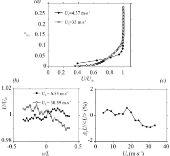
FIG. 2: Free stream characterization at the location of the Ahmed body, boundary layer profile on the floor(a), lateral velocity profile at z∗= 1/2 (b), right to left asymmetry (see text) of the lateral velocity profile vs. the main velocity (c).

on the floor of the free stream at the body location (say X = 260 mm from the leading edge of the ground plate and without the body) is shown in Fig. 2 for the two extreme main flow velocities of the explored range. The boundary layer profile at the lowest velocity has a Reynolds number based on the development length

ReX = 0.75 × 105 and suggests that it is laminar at the

lowest velocity. At the largest velocity, ReX = 5.72 × 105

and the shape suggests a turbulent boundary layer. For

both cases, the thickness never exceeds δ_0.99∗ = 0.1. The

laminar-turbulent transition occurs around 14 m·s−1, say

ReX = 2.42 × 105. However, this transition has no

mean-ing considermean-ing the flow around the Ahmed body whose presence produces pressure gradients at the ground wall that modifies drastically the boundary layer history com-pared to a development on the flat floor alone.

The spanwise spatial homogeneity is characterized

through the velocity measurements in Fig. 2(b).

Al-though the spatial inhomogeneity still remains below 0.4% in rms quantities, the streamwise velocity displays a small but significant shear whose sign depends upon the mean flow velocity. Figure 2(c) shows the difference between the mean velocity computed from the right hand side of the tunnel (y > 0) and the left hand side of the tunnel (y < 0). There is a velocity excess on the left hand side of the free stream of about 1% for mean flow

veloc-ities larger than 20 m·s−1. These symmetrical defects

in the free stream have to be acknowledged considering their induced bias in the onset of a symmetry breaking instability.

III. RESULTS

A. Global quantities for the near wake

The pressure distribution at the base of the body has been shown to be a relevant indicator [19, 20, 24, 25] of the large scale wake topology. As in [25], we will use the instantaneous barycentre of the base pressure distribu-tion, that we define as :

~ rb(yb, zb) = RR Base~r Cp(~r)dydz RR BaseCp(~r)dydz , (2)

It should be noted that for a massively separated wake flow as in the present case, the pressure of the base is always lower than the static pressure of the free stream meaning that the denominator in Eq. 2 is non-zero and al-ways negative. Figure 3(a,b) shows the two components of the base pressure barycentre. Its horizontal compo-nent in Fig. 3(a) clearly exhibits the bi-modal behavior. The two most probable horizontal positions observed at

y∗_b ' ±0.05 are associated with the two deflected wakes

fully characterized in [19]. They correspond to the two mirror RSB modes breaking the reflectional symmetry with respect of the plane y = 0 of the set-up. As it has already been shown in [19] the characteristic timescale to

4 switch between these modes is 2 to 3 orders of magnitude

larger than the natural timescale T∗ = 1 in non

dimen-sional units, (i.e. T = _UH

0). For the remainder of this

study, time series are low-pass filtered to focus on this

long time dynamics, with a cut-off frequency f∗

c = 2501

(say fc = 0.22 Hz at U0 = 4 m·s−1 to fc = 1.83 Hz at

U0 = 33 m·s−1). The filtered data are shown for the

barycentre coordinates in Fig. 3(c).

The most probable positions of the pressure barycentre are extracted from probability density functions (PDFs) such as the one presented in Fig. 4. The statistics are

performed over a duration fixed to 50 s, (τ∗ = 27500 at

U0 = 33 m·s−1 and τ∗ = 3300 at U0 = 4 m·s−1). The

choice of recording duration is a compromise between an accurate estimation of the position of the most proba-ble events and the high cost of time due to a parametric study involving changes in yaw angle, ground clearance and Reynolds number. As we can attest from Fig. 4, the most probable event positions are sufficiently well defined to investigate the parametric study of the stable branch solutions. Note that the chosen recording time

that evolves in the range τ∗ ∼ 3000 − 27500 leads

un-avoidably to weakly converged PDFs because of the long time dynamics associated with the RSB modes having a

characteristic timescale in the range τ∗∼ 100−1000 [19].

Hence, the weak convergence does not allow an accurate estimate of the value of the corresponding probability density.

Another global quantity of interest is the base suction −Cpb, where : Cpb = 1 S Z Z Base Cp(~r)dydz. (3)

The base suction is directly related to the form drag (see [26], [27] and references therein), the larger the base suc-tion, the larger the form drag. Note that the discrete pressure taps distribution at the base (Fig. 1c) will not lead to an exact measurement of the base suction but rather to a drag indicator.

B. Wake mode sensitivity to a yaw angle β and ground clearance C∗

Figure 5 shows the PDFs of the statistical variable

y_b∗, for 10 sets of experiments performed for the same

Reynolds number Re=146800. The grey levels of the

PDFs allow the most probable positions of the barycen-tre, which contains the main information, to be located.

For each set, the ground clearance C∗ _{is fixed and the}

yaw angle is varied within the range −1◦ < β < +1◦

in step of 0.1◦. By looking at the PDFs at the top of

Fig. 5 obtained for the ground clearance C∗ = 0.153, we

notice that two distinguished most probable positions,

symmetrically located at y∗+_b ' 0.05 and y∗−_b ' −0.05

are observable. These two positions are associated with the two stable mirror states and the values of y?±_b do not depend upon the yaw angle. When the ground clearance

zb * t* (a) yb * zb * yb* 0 5 10 15 0.1 0.05 0 -0.05 -0.1 t* (b) 0 5 10 15 0.1 0.05 0 -0.05 -0.1 t* (c) 0 5 10 15 0.1 0.05 0 -0.05 -0.1 ×103 ×103 ×103

FIG. 3: Time series of the base pressure barycenter coordi-nates (y∗b, z ∗ b), y ∗ b (a), z ∗ b (b) and filtered in (c). yb* 0.01 0.015 0.02 0.005 0 -0.05 -0.1 0 0.05 0.1 0.025 0.03 0.035 PDF

FIG. 4: Probability density function (PDF) of the horizontal coordinate y∗b of the base pressure barycenter computed from

the time serie in Fig. 3(c).

is decreased to C∗ = 0.09, similar observations can be

made except that now the two positions are not

symmet-rically located anymore. It emphasizes the sensitivity

to symmetry defects in the setup, especially related to the non-uniformity of the incoming flow as described in Fig. 2.

For slightly smaller C∗, the two states become hardly

distinguishable and instead, a continuous change in the pressure barycentre coordinate is observed.

−1 −0.5 0 0.5 1 −0.14 0 0.14 −0.14 0 0.14 −0.14 0 0.14 −0.14 0 0.14 yb* yb* yb* yb* β (°) C*_{= 0.153} C*_{= 0.125} C*_{= 0.097} C*_{= 0.09} C*_{= 0.083} C*_{= 0.08} C*_{= 0.076} C*_{= 0.073} C*_{= 0.056} C*_{= 0.066}

FIG. 5: Evolution of the probability density function, PDF(yb∗) in grey levels (the darker, the larger the PDF) for

U0 = 30.58 m·s−1 with the yaw angle β and for different

ground clearances C∗.

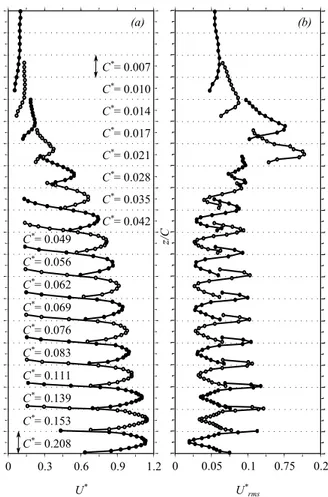
ground clearance is now investigated. Velocity profiles are then measured 2 mm behind the body using a clas-sical hot wire probe, in the mid plane y = 0 for different

ground clearances C∗. They are all presented in Fig. 6 as

z/C vs. the velocity with a vertical shift for clarity. For large ground clearances, C∗ > 0.04, velocity profiles are well established and present a relatively parabolic shape. The velocity fluctuations are maximum (Fig. 8b) on the top side of the profiles which corresponds to the free mix-ing layer, and on the bottom side that corresponds to

C*_{= 0.153} C*_{= 0.208} C*_{= 0.139} C*_{= 0.111} C*_{= 0.083} C*_{= 0.076} C*_{= 0.069} C*_{= 0.062} C*_{= 0.049} C*_{= 0.056} C*_{= 0.042} C*_{= 0.035} C*_{= 0.028} C*_{= 0.021} C*_{= 0.017} C*_{= 0.014} C*_{= 0.010} C*_{= 0.007} 0 0.3 0.6 0.9 1.2 0 0.05 0.1 0.75 0.2 U* _U* rms z/C (a) (b)

FIG. 6: Characterization of the underbody flow using hot wire anemometer measurements, 2 mm behind the body in the y = 0 plane. The hot wire is oriented to be sensitive to the longitudinal velocity u(t). (a) : z/C vs. the time averaged non-dimensional velocity U∗ = u∗_{. (b) Fluctuating velocity}

defined as Urms∗ =

q

(u∗_{− U}∗₎2_.

the boundary layer on the floor. For ground clearances

smaller than C∗ < 0.04, there is no established

under-body flow and a transition with high velocity fluctuations

is observed for C∗= 0.021.

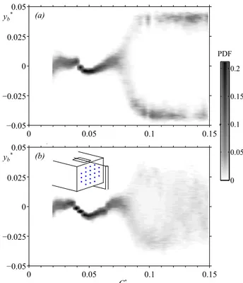
To study the two stable solutions of the bifurcated states, we chose to explore the wake positions for the

two yaw angles β = −0.4◦in Fig. 7(a) and β = +0.4◦ in

Fig. 7(b). The negative (resp. positive) yaw angle allows exploration of the branch y∗+_b (resp. y∗−_b ) correspond-ing to the positive (resp. negative) part of PDF(y∗_b). As

can be seen, the system explores preferentially the y∗+

branch near the bifurcation point which is an evidence for an imperfect bifurcation. In addition, we never no-ticed any hysteretic effect by working with increasing or decreasing control parameters, which reinforces the su-percritical character of the bifurcation. For both PDF branches, the position of the local maxima are extracted (plotted as white lines in Fig. 7a and b). This technique of extraction will be repeated in the following to study the Reynolds number effect on the bifurcation diagram.

6 yb* 0 0.025 0.05 −0.025 −0.05 0.05 0 0.1 (a) 0.15 yb* 0 0.025 0.05 −0.025 −0.05 0.05 0 0.1 (b) 0.15 U*_{, U}* rms C* 0.6 0.9 1.2 0.3 0 0.05 0 0.1 (c) 0.15

FIG. 7: Probability density functions, PDF(yb∗) in grey levels

for U0 = 30.58 m·s−1 vs. the ground clearance C∗, for (a)

with the yaw angle β = −0.4◦ and (b) with a yaw angle β = +0.4◦. The white lines represent the most probable position and correspond in (a, continuous line) to the stable branch y∗+b and in (b, dashed line) to the other stable branch y

∗−

b .

In (c) are reported the maximum of the profiles measured in Fig. 6, mean velocity U∗(empty circles) and fluctuation Urms∗

(black filled circles).

Figure 7(c) displays the maximum values of the pro-files measured in Fig. 6. It is clear from these results that

the underbody flow is already well established, about U0

at the pitchfork point of the bifurcation observed around

C∗ _{∼ 0.075. Hence, the large velocity fluctuations}

ob-served at C∗= 0.021 occurs at a too small ground

clear-ance to be associated with the instability threshold of the RSB states.

C. Bifurcation threshold with Reynolds number

Nine experiments with different Reynolds numbers have been conducted with exactly the same protocol as for the previous experiment. All of the bifurcation

di-agrams obtained by superimposing the branch y∗+ and

y∗− are shown in Fig. 8. We can see clear imperfect

pitchfork bifurcations due to some symmetry defects be-fore and at the bifurcation point. As said above, these imperfections are likely to be explained by the free stream properties characterized in Fig. 2. The bifurcation point, defines as the crossing point between the two branches, appears to depend on the Reynolds number, and its

de-pendency is shown in Fig. 9. The uncertainty about C_c∗

is estimated to be ±0.0025 reflecting the measurements displayed in Fig. 8(a).

The critical ground clearance C_c∗ is a slow decreasing

function of the critical Reynolds number Rec, similar to

the power law Re−1/6c in the range of our experiments.

D. Toward a stabilization using passive control

We now investigate the possibility for the existence of an unstable branch solution, corresponding to the prolon-gation of the symmetric state after the bifurcation point. The idea is to apply the passive control technique first in-troduced by [28] to stabilize the K´arm´an instability in the laminar wake of a circular cylinder. It has been shown for the present configuration in [24] to efficiently eliminate the bi-modal behavior of the turbulent wake. It consists in a steady disturbance technique by introducing inside the recirculating bubble a vertical cylinder, having the

same height as the body with a diameter d∗_{= 0.083. We}

placed the control cylinder at the best location obtained

in [24], say y∗ = 0 and x∗ = 0.52. Two thin rods, as

depicted in Fig.10(b), support the control cylinder. In order to characterize the effect of the control cylinder only, a bifurcation diagram has been performed with the body and the two thin rods as a function of the ground clearance. It is shown in Fig.10(a). Because of the thick-ness of the rod under the body, the ground clearance is

limited for low values to C∗ = 0.035. The observed

bi-furcation, very similar to the one obtained without the rods (Fig.7), attests from the neutrality of the support-ing system. Furthermore, it has to be mentioned that the bifurcation in Fig.10(a) is obtained for only one yaw angle. It has been especially adjusted in order to have the best equiprobable exploration of the two states at the largest ground clearance. In this condition, we see that both branches are randomly explored after the bi-furcation point, leading to the bistable dynamics of the wake.

When the control cylinder is placed between the two rods, the bifurcation diagram before the pitchfork point remains unaltered compared to that of the reference, while after the pitchfork point the two branches are re-placed by a continuum of uniform density probability

0 0.05 0.1 0.15 −0.1 0 0.1 −0.1 0 0.1 −0.1 0 0.1 yb* C*

FIG. 8: Bifurcation diagrams vs. the ground clearance ob-tained with different Reynolds numbers, from bottom to top : Re=1.78×104, 2.89×104, 3.95×104, 5.05×104, 6.1×104, 8.27× 104, 1.04 × 105, 1.32 × 105, 1.6 × 105. For each Reynolds num-ber, the branches are extracted from the most probable posi-tion of the barycentre obtained from β = −0.4◦(blue circles) and β = +0.4◦(white circles) as in Fig. 7(a) and (b).

over values of y?_{included within y}?±

b , yet excluding y

?± b .

At this point it is difficult to argue whether the system is actually stabilized since there is no most probable

posi-tion around y∗= 0. However the system is definitely not

bi-modal anymore. This simple experiment is promising since passive control can be considerably improved using active control. We are confident that the latter will be the good strategy to stabilize the wake.

Although the suppression of the lateral force can be achieved by stabilizing the flow, it remains interesting to look at the effect of a stabilization on the base suction and hence the drag. The base suction as defined in Eq.3 is shown in Fig.11. The dashed line refers to the refer-ence case, it displays large variations of the base suction

Cc *

10-1

104 ₁₀5

Rec

FIG. 9: Threshold of the bifurcation, critical ground clearance vs. critical Reynolds number.

PDF 0 0.05 0.1 0.15 0.2 yb* 0 0.025 0.05 −0.025 −0.05 0.05 0 0.1 (a) 0.15 yb* 0 0.025 0.05 −0.025 −0.05 0.05 0 0.1 (b) 0.15 C*

FIG. 10: Probability density functions, PDF(yb∗) in grey levels

for U0 = 30.58 m·s−1 vs. the ground clearance C∗, for (a)

with the yaw angle β = −0.4◦and (b) with a yaw angle β = +0.4◦. The white lines represent the most probable position and correspond in (a, continuous line) to the stable branch y_b∗+and in (b, dashed line) to the other stable branch y_b∗−.

coefficient due to the development of the underbody flow as already described in [20] and characterized in Fig. 6.

However, the abrupt change observed for C∗ ∼ 0.09 is

clearly ascribed to the pitchfork point, indicating that the presence of the RSB modes are creating additional base suction and then drag. By stabilizing the wake, one would expect the base suction coefficient to decrease in the continuity of its evolution before the pitchfork point. It is actually what is observed when the control cylinder

8 −Cpb 0.27 0.28 0.29 0.26 0.25 0.05 0 0.1 0.15 C*

ref.

control

FIG. 11: Base pressure suction vs. the ground clearance for (dashed line) the reference case of Fig. 10(a) and for (contin-uous line) the controlled case of Fig. 10(b).

is added, the base suction follows the same variations as for the reference case. After the instability threshold, a significant reduction is observed. This passive control experiment is encouraging as a new strategy for drag re-duction of 3D turbulent wakes.

E. Flow visualizations

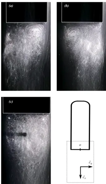
We turn now to an illustrative experiment of flow visu-alization realized in a water tunnel. The model is a 1:2.66 scale of the one used above. The test section of the

tun-nel is 80 × 150 mm and the flow speed 6 m·s−1. The

Reynolds number is 216000, and the ground clearance is

set to C∗ _{= 0.1. The yaw angle is accurately adjusted}

to obtain the bistable dynamics of the two RSB states. We present in Fig. 12, some pictures extracted from a long time movie showing the random switching between

the y+_b stable solution shown in (a) and the y_b− stable

solution shown in (b). The two wake states present a mirror symmetry, with an intense circular recirculation clearly visible on the right hand side in Fig. 12(a) and symmetrically on the left hand side in Fig. 12(b). The low pressure barycentre position is on the same side as this intense recirculation. These flow visualizations are in total agreements with the velocity field measurements of the RSB modes in [19]. When a vertical control cylin-der is added as in paragraph III D, a symmetric wake is observed without any intense recirculations.

IV. CONCLUSIVE REMARKS

The wake of a square-back body at the proximity of a ground wall undergoes a pitchfork bifurcation in the tur-bulent regime from a symmetric turtur-bulent wake toward two asymmetric turbulent wakes. The phase diagram in Fig. 9 indicates that the critical ground clearance is a slow decreasing function of the critical Reynolds num-ber. Thus, the bifurcation is also observable for a given

(a) (b)

(c)

o

FIG. 12: Flow visualization performed in a water tunnel using bubbles appearing white against a black background. The flow Reynolds number is Re = 216000 at a ground clearance C∗= 0.1. The drawing shows the visualization area depicted by a dashed rectangle at the rear of the Ahmed body. The obturation time of the camera is τ∗ = 3, say 3 times larger than the convective time H/U0 and captures the dynamics

at this timescale. In (a), RSB mode of the branch y+_b, in (b) its mirror counterpart: the RSB mode of the branch y_b−. Wake controlled with a vertical control cylinder (diameter d∗= 0.107).

ground clearance as the Reynolds number is increased. The smaller the ground clearance the larger the Reynolds number for the transition. At the threshold of the in-stability (pitchfork point), the underbody flow

magni-tude is approximately U0 (see Fig. 7c) indicating that

the bifurcation is not related to a flow transition in the ground clearance. Following the idea of Grandemange et al. [20], the crucial ingredient for the symmetry break-ing is the ratio between the separatbreak-ing distances of the vortex sheets produced by the separation at the rectan-gular base (it is also the result of the stability analysis by

Marquet and Larsson [22] for a rectangular plate facing a uniform flow in the laminar regime). The inviscid condi-tion at the ground wall, that can be justified for large Re flow, is equivalent to a mirror flow. In the absence of the underbody flow, the top vortex sheet emerging from the square-back body is then facing its symmetric counter part at a distance that is the double of the body height, 2H. In the case of an underbody flow, a second vortex sheet emerges from the bottom trailing edge of the body and the separating distance with the top vortex sheet is now H. For the primary case, the aspect ratio is twice the second case and does not allow the symmetry break-ing instability at the given width W of the base [20]. Hence the large Reynolds number bifurcation appears to be related to a stabilizing geometrical parameter. One may wonder if an equivalent explanation can be tested

on the transition obtained with the von-K´arm´an swirling

flow geometry.

There are some interesting applications for flow control of 3D turbulent wakes. For instance, the pioneering tech-nique of Strykowski and Sreenivasan [29] to stabilize the

periodic laminar K´arm´an instability toward the steady

state is also efficient to stabilize the turbulent RSB mode toward a symmetric wake mode. In addition to the flow studied here, it is known that the turbulent wake of ax-isymmetric bodies develops symmetry breaking modes as well [25, 30]. Thus the stabilization toward the symmet-ric unstable mode might be a relevant strategy for drag and lateral force reduction in many applications with po-tentially a low energetic cost and offers promising future development.

Acknowledgments

The authors are grateful to Romain Monchaux for

use-ful discussions about the von-K´arm´an swirling flow and

thankful to John Wrightson for his critical reading of the manuscript. This work benefited from the financial support of the Labex LaSIPS in the framework of the TURBFORK project.

[1] U. Frisch, Turbulence (Cambridge University Press, 1996).

[2] H. Schlichting and K. Gersten, Boundary layer theory (Springer Verlag, 2000).

[3] P. Bearman, Journal of Fluid Mechanics 37, 577 (1969). [4] E. Achenbach and E. Heinecke, Journal of Fluid

Mechan-ics 109, 239 (1981).

[5] G. Schewe, Journal of Fluid Mechanics 133, 265 (1983). [6] G. Schewe, Journal of Fluid Mechanics 172, 33 (1986). [7] C. Farell and J. Blessmann, Journal of Fluid Mechanics

136, 375 (1983).

[8] J. J. Miau, H. W. Tsai, Y. J. Lin, J. K. Tu, C. H. Fang, and M. C. Chen, Experiments in Fluids 51, 949 (2011). [9] Y.-J. Lin, J.-J. Miau, J.-K. Tu, and H.-W. Tsai, AIAA

Journal 49, 1857 (2011).

[10] O. Cadot, A. Desai, S. Mittal, S. Saxena, and B. Chan-dra, Physics of Fluids 27, 014101 (2015).

[11] F. Ravelet, L. Marie, A. Chiffaudel, and F. Daviaud, Physical Review Letters 93, 164501 (2004).

[12] A. de la Torre and J. Burguete, Physical Review Letters 99, 054101 (2007).

[13] F. Ravelet and F. Chiffaudel, A.and Daviaud, Journal of Fluids Mechanics 601, 339 (2008).

[14] P.-P. Cortet, A. Chiffaudel, F. Daviaud, and B. Dubrulle, Physical Review Letters 105, 214501 (2010).

[15] P.-P. Cortet, E. Herbert, A. Chiffaudel, F. Daviaud, B. Dubrulle, and V. Padilla, Journal of Statistical Mechanics-Theory and Experiment P07012 (2011). [16] C. Nore, L. Tuckerman, O. Daube, and S. Xin, Journal

of Fluid Mechanics 477, 51 (2003).

[17] C. Nore, L. Witkowski, E. Foucault, J. Pecheux, O. Daube, and P. Le Quere, Physics of Fluids 18, 054102 (2006).

[18] M. Grandemange, M. Gohlke, and O. Cadot, Physical Review E 86, 035302 (2012).

[19] M. Grandemange, M. Gohlke, and O. Cadot, Journal of Fluid Mechanics 722, 51 (2013).

[20] M. Grandemange, M. Gohlke, and O. Cadot, Physics of Fluids 25, 095103 (2013).

[21] B. Pier, Journal of Fluid Mechanics 603, 39 (2008). [22] O. Marquet and M. Larsson, European Journal of

Me-chanics B/Fluids 49, 400 (2014).

[23] S. Ahmed, G. Ramm, and G. Faitin, SAE Technical Pa-per Series 840300 (1984).

[24] M. Grandemange, M. Gohlke, and O. Cadot, Journal of Fluid Mechanics 752, 439 (2014).

[25] G. Rigas, A. Oxlade, A. Morgans, and J. Morrison, Jour-nal of Fluid Mechanics 755, 159 (2014).

[26] A. Roshko, Journal of Wind Engineering and Industrial Aerodynamics 49, 79 (1993).

[27] C. Apelt and G. West, Journal of Fluid Mechanics 71, 145 (1975).

[28] P. Strykowski and K. Sreenivasan, Journal of Fluid Me-chanics 218, 71 (1990).

[29] P. Strykowski and K. Sreenivasan, in AIAA Shear Flow Control Conference (1985).

[30] M. Grandemange, M. Gohlke, and O. Cadot, Experi-ments in fluids 55, 1 (2014).