EUROPEAN ORGANIZATION FOR NUCLEAR RESEARCH (CERN)
CERN-EP-2018-059 LHCb-PAPER-2018-004 31 July 2018
Evidence for the decay
B
s
0
→ K
∗0
µ
+
µ
−
LHCb collaboration†
Abstract
A search for the decay Bs0→ K∗0µ+µ−is presented using data sets corresponding to
1.0, 2.0 and 1.6 fb−1 of integrated luminosity collected during pp collisions with the
LHCb experiment at centre-of-mass energies of 7, 8 and 13 TeV, respectively. An ex-cess is found over the background-only hypothesis with a significance of 3.4 standard
deviations. The branching fraction of the Bs0→ K∗0µ+µ−decay is determined to be
B(B0
s→ K∗0µ+µ−) = [2.9 ± 1.0 (stat) ± 0.2 (syst) ± 0.3 (norm)] × 10−8, where the
first and second uncertainties are statistical and systematic, respectively. The third uncertainty is due to limited knowledge of external parameters used to normalise the branching fraction measurement.
Published in JHEP 07 (2018) 020
c
2018 CERN for the benefit of the LHCb collaboration, CC-BY-4.0 licence.
†Authors are listed at the end of this paper.
1
Introduction
The decay B0
s→ K∗(892)0µ+µ−, hereafter referred to as Bs0→ K∗0µ+µ−, proceeds via a
b → d flavour-changing neutral-current (FCNC) transition. The leading contributions to the amplitude of the decay correspond to loop Feynman diagrams and involve the off-diagonal element Vtd of the Cabibbo-Kobayashi-Maskawa (CKM) quark-mixing matrix.
This process is consequently rare in the Standard Model of particle physics (SM). New particles predicted by extensions of the SM can enter in competing diagrams and can significantly enhance or suppress the rate of the decay, see for example Refs. [1, 2]. Form-factor computations for the Bs0 → K∗0 transition have been made using light-cone sum
rule [3, 4] and lattice QCD [5] techniques. Standard Model predictions for the branching fraction of the decay are in the range 3–4 × 10⁻⁸ [6–8].
The observation of the rare b → d`+`− FCNC decays B+ → π+µ+µ− and
Λ0 b→ pπ
−µ+µ− has been previously reported by the LHCb collaboration in Refs. [9]
and [10], respectively. Evidence for the decay B0→ π+π−µ+µ− has also been established
in Ref. [11]. The decay Bs0→ K∗0µ+µ− has not yet been observed. The measured ratio
of the B+→ π+µ+µ− and B+→ K+µ+µ− branching fractions has also been used to
determine the ratio of CKM elements |Vtd/Vts| [12], exploiting correlations between the
B → K and B → π form-factors in lattice computations. A similar approach could, in the future, be applied to the ratio of the B0
s→ K
∗0µ+µ− and B0→ K∗0µ+µ− decay rates [13].
The decay B0→ K∗0µ+µ−, which involves a b → s`+`− transition, has been studied
extensively by BaBar, Belle, CDF and by the LHC experiments [14–19]. The rate of the decay appears to be systematically lower than current SM predictions. Global analyses of b → s processes favour a modification of the SM at the level of 4 to 5 standard deviations [20–24]. Similar studies of b → d processes are important to understand the flavour structure of the underlying theory.
This paper presents a search for the decay B0
s → K
∗0µ+µ−, where the inclusion of
charge-conjugate processes is implied throughout, using data collected with the LHCb experiment in pp collisions during Runs 1 and 2 of the LHC. The data set used in this paper is as follows: 1.0 fb−1 of integrated luminosity collected at a centre-of-mass energy of 7 TeV during Run 1; 2.0 fb−1 of integrated luminosity collected at a centre-of-mass energy of 8 TeV during Run 1; and 1.6 fb−1 of integrated luminosity collected at a centre-of-mass energy of 13 TeV during Run 2. Section 2 of this paper describes the LHCb detector and the experimental setup used for the analysis. Section 3 outlines the selection processes used to identify signal candidates. Section 4 describes the method used to estimate the number of B0
s→ K
∗0µ+µ− decays in the data set. Section 5 describes the determination of
the Bs0→ K∗0µ+µ− branching fraction, normalising the number of observed signal decays
to the number of B0→ J/ψ K∗0 decays present in the data set. Section 6 discusses sources
of systematic uncertainty on the B0
s→ K
∗0µ+µ− branching fraction. Finally, conclusions
are presented in Sec. 7.
2
Detector and simulation
The LHCb detector [25, 26] is a single-arm forward spectrometer covering the pseudorapidity range 2 < η < 5, designed for the study of particles containing b or c quarks. The detector includes a high-precision tracking system consisting of a
silicon-strip vertex detector surrounding the pp interaction region [27], a large-area silicon-silicon-strip detector located upstream of a dipole magnet with a bending power of about 4 Tm, and three stations of silicon-strip detectors and straw drift tubes [28] placed downstream of the magnet. The tracking system provides a measurement of momentum, p, of charged particles with a relative uncertainty that varies from 0.5% at low momentum to 1.0% at 200 GeV/c. The minimum distance of a track to a primary vertex (PV), the impact param-eter (IP), is measured with a resolution of (15 + 29/pT) µm, where pT is the component of
the momentum transverse to the beam, in GeV/c. Different types of charged hadrons are distinguished using information from two ring-imaging Cherenkov detectors [29]. Photons, electrons and hadrons are identified by a calorimeter system consisting of scintillating-pad and preshower detectors, an electromagnetic calorimeter and a hadronic calorimeter. Muons are identified by a system composed of alternating layers of iron and multiwire proportional chambers [30].
The online event selection is performed by a trigger [31]. The trigger consists of a hardware stage, based on information from the calorimeter and muon systems, followed by a software stage, which applies a full event reconstruction. The signal candidates are required to pass through a hardware trigger that selects events containing at least one muon with pT greater than 1 to 2 GeV/c, depending on the data-taking conditions. The
software trigger requires a two-, three- or four-track secondary vertex with a significant displacement from any primary pp interaction vertex. At least one charged particle must have a large transverse momentum pT > 1 GeV/c and be inconsistent with originating
from a PV. A multivariate algorithm [32] is used for the identification of secondary vertices consistent with the decay of a b hadron.
Samples of simulated B0
s → K∗0µ+µ−, B0 → K∗0µ+µ−, Bs0 → J/ψ K∗0 and
B0→ J/ψ K∗0 decays are used to develop an offline event selection and to determine
the efficiency to reconstruct the B0 and B0
s candidates in the different data-taking periods.
In the simulation, pp collisions are generated using Pythia [33] with a specific LHCb configuration [34]. Decays of hadronic particles are described by EvtGen [35], in which final-state radiation is generated using Photos [36]. The interaction of the generated par-ticles with the detector, and its response, are implemented using the Geant4 toolkit [37] as described in Ref. [38]. Data-driven corrections are applied to the simulation to account for mismodelling of the detector occupancy and of the B0
(s) meson production kinematics.
The particle identification (PID) performance is measured from data using calibration samples [26].
3
Candidate selection
Signal candidates are formed by combining a K∗0 candidate with two oppositely charged tracks, which are identified as muons by the muon system. The K∗0 meson is reconstructed through its decay to the K−π+ final state with invariant mass within ±70 MeV/c2 of the known K∗(892)0 mass [39]. The muon pair is required to have an invariant mass squared
in the range 0.1 < q2 < 19.0 GeV2/c4, excluding the region 12.5 < q2 < 15.0 GeV2/c4
dominated by the ψ(2S) resonance. Candidates in the region 8.0 < q2 < 11.0 GeV2/c4, which are dominated by decays via a J/ψ resonance, are treated separately in the analysis. The remaining candidates include B0
s meson decays that produce a dimuon pair through
threshold, which are inseparable from the short-distance component of the decay. These are considered part of the signal in the analysis.
The selection process used in this analysis is similar to that described in Ref. [18]. The four charged tracks are required to each have a significant IP with respect to all PVs in the event and to be consistent with originating from a common vertex. The B0
(s)
meson candidate is required to be consistent with originating from one of the PVs in the event and its decay vertex is required to be well separated from that PV. The kaon and pion candidates must also be identified as kaon-like and pion-like by a multivariate algorithm [26] based on information from the RICH detectors, tracking system and calorimeters. The PID requirements are chosen to maximise the sensitivity to a SM-like B0
s→ K
∗0µ+µ− signal.
To improve the resolution on the reconstructed K−π+µ+µ− invariant mass, m(K−π+µ+µ−), candidates with an uncertainty larger than 22 MeV/c2 on their mea-sured mass are rejected. The opening angle between every pair of final-state particles is also required to be larger than 5 mrad in the detector. This requirement removes a possible source of background that arises when the hits associated to a given charged particle are mistakenly used in more than one reconstructed track. A kinematic fit is also performed, constraining the candidate to originate from its most likely production vertex [40]. In the kinematic fit of candidates with q2 in the J/ψ mass window, the dimuon pair is also constrained to the known J/ψ mass. This mass constraint improves the resolution in m(K−π+µ+µ−) for candidates involving an intermediate J/ψ resonance decay by a factor
of two.
Signal candidates are further classified using an artificial neural network [41]. The neural network is trained using a sample of simulated B0→ K∗0µ+µ− decays as a proxy
for the signal decay. Candidates in data with m(K−π+µ+µ−) > 5670 MeV/c2 are used as a background sample. This sample is predominantly comprised of combinatorial background, where uncorrelated tracks from the event are mistakenly combined. The neural network uses the following variables related to the topology of the B0(s) meson decay: the angle between the reconstructed momentum vector of the B(s)0 meson and the vector connecting the PV and the decay vertex of the B(s)0 candidate; the IP, pT and proper decay time of
the B(s)0 candidate; the vertex fit quality of the B(s)0 decay vertex and of the dimuon pair; the minimum and maximum pT of the final-state particles and for the Run 1 data set a
measure of the isolation of the final-state particles in the detector. It has been verified that the distribution of the variables used as input to, and the output distribution from, the classifier agree between the simulation and the data. The output of the neural network is transformed such that it is uniform in the range 0–1 on the signal proxy. Candidates with neural network response below 0.05 are rejected in the subsequent analysis. This requirement removes a background-dominated part of the data sample. The neural network response is validated on simulated B0→ K∗0µ+µ− and B0
s→ K
∗0µ+µ− decays to ensure
that it does not introduce any bias in m(K−π+µ+µ−).
Finally, a number of vetoes are applied to reject specific sources of background. Signal candidates are rejected if the pion candidate has a nonnegligible probability to be a kaon and if the K+K− invariant mass, after assigning the kaon mass to the pion candidate, is consistent within 10 MeV/c2 of the known φ(1020) meson mass. This veto removes 98% of
B0
s→ φµ+µ
− decays inside the φ(1020) mass window. Candidates are also rejected if the
muon mass hypothesis to the kaon or pion candidate, are consistent with that of a J/ψ or ψ(2S) meson (within ±60 MeV/c2 of their known masses).
4
Signal yields
In order to maximise sensitivity to a B0
s→ K
∗0µ+µ− signal, candidates are divided into
regions of neural network response. The candidates are also divided based on the two data-taking periods, Run 1 and Run 2. Four regions of neural network response are selected for each data-taking period, each containing an equal amount of expected signal decays. The yield of the B0
s→ K
∗0µ+µ−decay is determined by performing a simultaneous
unbinned maximum likelihood fit to the m(K−π+µ+µ−) distribution of the eight resulting subsets of the data.
In the likelihood fit, the signal lineshape of both the B0 and the B0
s → K
∗0µ+µ−
decays is described by the sum of three functions: a Gaussian function with a power-law tail on the lower-side of its peak, used to describe final-state radiation and energy loss in the detector; a Gaussian function with a power-law tail on the upper-side of its peak, used to describe the non-Gaussian tails of the signal mass distribution at large masses; and an additional Gaussian function to account for differences in the per-candidate resolution of the reconstructed mass. The two functions with power-law tails share a common width and all three functions share a common peak position. The Bs0 peak position is displaced from that of the B0 by 87.5 MeV/c2 [42]. The relative fractions of each function are fixed from fits to simulated B0 and B0
s→ K
∗0µ+µ− decays. The widths of the functions and
all of the tail parameters are also fixed from the simulation, except for an overall scaling of the widths and of the tail parameters to allow for potential data-simulation differences. The peak position and these scale factors are obtained from a fit to candidates with the dimuon in the J/ψ mass window, where the mass constraint on the dimuon mass has not been applied. The result of this fit is shown in the appendix in Fig. 4. In the fit to the data, the widths vary from their values in the simulation by 10 to 15%. The turn-on point of the upper tail (relative to the width of the distribution) is found to be consistent between data and simulation.
After applying the selection procedure, the background predominately comprises combinatorial background. The combinatorial background is described in the fit by a separate exponential function in each subset of the data. A number of other sources of background are accounted for in the fit. The decay B0→ K∗0µ+µ− forms a source of
background if the kaon is mistakenly identified as the pion and vice versa. The shape of this background is taken from the simulation. The yield of the background is constrained relative to that of the B0 → K∗0µ+µ− decay based on measurements of the
kaon-to-pion and kaon-to-pion-to-kaon misidentification probabilities in the PID calibration samples. The decay Λ0b→ pK−µ+µ− forms a source of background if the final-state hadrons are
misidentified. This background is constrained from a control region in the data, by modifying the PID requirements on the candidates to preferentially select pK− rather than K−π+ combinations. The shape of this background is modelled in the fit by Crystal Ball functions. The yield in each subset of the data is constrained using the proton and kaon identification and misidentification probabilities determined from the PID calibration samples. The decay B−→ K−µ+µ− forms a source of background if a pion from the
background contribution from B−→ K−µ+µ− decays is determined from a control region
in the data, by selecting candidates with a K−µ+µ− invariant mass that is consistent
with the known B− mass. This background is only visible for the candidates with q2 in the J/ψ mass region. The shape of the background in the fit is modelled by Crystal Ball functions. Several other sources of background are considered but are found to have a negligible contribution to the fit. These sources include semileptonic decays of b hadrons via intermediate open-charm states and fully hadronic b-hadron decays. The background from semileptonic decays is predominantly reconstructed at low m(K−π+µ+µ−) and does
not contribute to the analysis. Fully hadronic b-hadron decays contribute at the level of 1 to 2 candidates at masses close to the known Bs0 mass. This background is neglected in the analysis but is considered as a source of systematic uncertainty in Sec. 6.
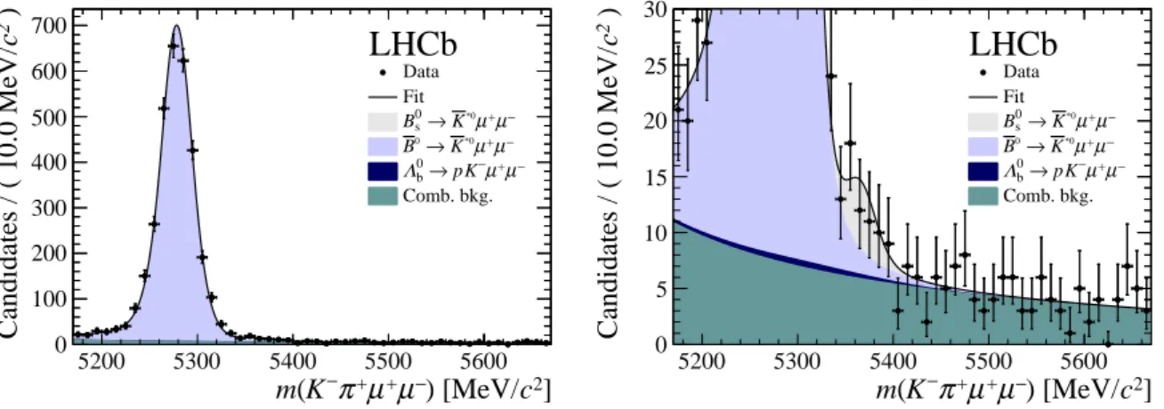
Figure 1 shows the fit to the candidates, where the result of the fit in the three most signal-like neural network response bins for each data-taking period has been combined. Candidates in the least signal-like bin are not included. This bin has a much higher level of combinatorial background and would visually obscure any B0s signal. The dominant contribution in the fit is the B0→ K∗0µ+µ− decay. Figure 2 shows the fit to the mass-constrained candidates in the J/ψ mass region, also with the three highest neural network response bins for each data taking period combined. In this fit, a small background component from B0→ K∗0µ+µ− decays is included. This background has the same final state but is constrained to the wrong dimuon mass and becomes a broad component in the fit. The fit results in individual bins of neural network response are shown in the appendix in Figs. 5 and 6. Summing over the bins of neural network response and data-taking periods, the yields are: 627 244 ± 837 for the B0→ J/ψ K∗0 decay, 5730 ± 94
for the B0
s→ J/ψ K∗0 decay, 4157 ± 72 for the B0→ K∗0µ+µ− decay, and 38 ± 12 for the
Bs0→ K∗0µ+µ− decay. No correction has been made to these yields to account for cases
where the K−π+ system does not originate from a K∗(892)0 decay. Contamination from
non-K∗0 decays is discussed further in Sec. 5. Using Wilks’ theorem, and a likelihood ratio test between the signal-plus-background and the background-only hypothesis, the significance of the B0
s→ K
∗0µ+µ− yield is determined to be p−2 log(L
S+B/LB) = 3.4
standard deviations. The signal significance has been validated using pseudoexperiments generated under the null hypothesis. This includes the systematic uncertainties on the yield discussed in Sec. 6. Figure 3 shows the variation of the log-likelihood of the simultaneous fit as a function of the B0
s→ K∗0µ+µ− yield.
5
Results
The branching fraction of the B0
s→ K
∗0µ+µ− decay is determined with respect to that of
B0→ J/ψ K∗0 according to B(Bs0→ K∗0µ+µ−) = B(B0→ J/ψ K∗0)B(J/ψ → µ+µ−) × fd fs N (B0 s → K ∗0µ+µ−) ε(B0 s → K∗0µ+µ−) ε(B0 → J/ψ K∗0) N (B0 → J/ψ K∗0). (1)
Here, N is the yield for a given decay mode determined from the fit to m(K−π+µ+µ−) or m(J/ψ K−π+) and ε is the efficiency to reconstruct and select the given decay mode. The
5200 5300 5400 5500 5600 ] 2 c ) [MeV/ − µ + µ + π − K ( m 0 100 200 300 400 500 600 700 ) 2 c Candidates / ( 10.0 MeV/
LHCb
Data Fit − µ + µ *0 K → s 0 B − µ + µ *0 K → 0 B − µ + µ − K p → b 0 Λ Comb. bkg. 5200 5300 5400 5500 5600 ] 2 c ) [MeV/ − µ + µ + π − K ( m 0 5 10 15 20 25 30 ) 2 c Candidates / ( 10.0 MeV/LHCb
Data Fit − µ + µ *0 K → s 0 B − µ + µ *0 K → 0 B − µ + µ − K p → b 0 Λ Comb. bkg.Figure 1: Distribution of reconstructed K−π+µ+µ−invariant mass of candidates outside the J/ψ
and ψ(2S) mass regions, summing the three highest neural network response bins of each run condition. The candidates are shown (left) over the full range and (right) over a restricted vertical
range to emphasise the B0
s→ K∗0µ+µ− component. The solid line indicates a combination of
the results of the fits to the individual bins. Components are detailed in the legend, where they are shown in the same order as they are stacked in the figure. The background from misidentified
B0→ K∗0µ+µ− decays is included in the B0→ K∗0µ+µ− component.
5200 5300 5400 5500 5600 ] 2 c ) [MeV/ + π − K ψ J/ ( m 0 10 20 30 40 50 60 3 10 × ) 2 c Candidates / ( 2.5 MeV/
LHCb
Data Fit *0 K ψ J/ → s 0 B *0 K ψ J/ → 0 B − µ + µ *0 K → 0 B − K p ψ J/ → b 0 Λ + K ψ J/ → + B Comb. bkg. 5200 5300 5400 5500 5600 ] 2 c ) [MeV/ + π − K ψ J/ ( m 0 100 200 300 400 500 600 700 800 ) 2 c Candidates / ( 2.5 MeV/LHCb
Data Fit *0 K ψ J/ → s 0 B *0 K ψ J/ → 0 B − µ + µ *0 K → 0 B − K p ψ J/ → b 0 Λ + K ψ J/ → + B Comb. bkg.Figure 2: Distribution of reconstructed J/ψ K−π+ invariant mass of the candidates in the J/ψ
mass region summing the three highest neural network response bins of each run condition, shown (left) over the full range and (right) over a restricted vertical range to emphasise the
Bs0→ J/ψ K∗0 component. The solid line indicates a combination of the results of the fits to the
individual bins. Components are detailed in the legend, where they are shown in the same order
as they are stacked in the figure. The background from misidentified B0→ J/ψ K∗0 decays is
included in the B0→ J/ψ K∗0 component.
The efficiency to trigger, reconstruct and select each of the decay modes is determined from the simulation after applying the data-driven corrections. The efficiency for the B0
s→ K
∗0µ+µ− decay is corrected to account for events in the vetoed q2 regions following
the same prescription as Ref. [19]. The efficiency corrected yields are further corrected for contamination from decays with the K−π+ system in an S-wave configuration. For
the decay B0
s→ J/ψ K
∗0, the S-wave fraction of F
S(B0→ J/ψ K∗0) = (6.4 ± 0.3 ± 1.0)%
0 20 40 60 80
]
−µ
+µ
*0K
→
s 0B
[
N
0 2 4 6 8 10 12L
log
∆
2
−
LHCb
Figure 3: Change in log-likelihood from the simultaneous fit to the candidates in the two data-taking periods and the different bins of neural network response, as a function of the
Bs0→ K∗0µ+µ−yield. Systematic uncertainties on the yield have been included in the likelihood.
is unknown but it is assumed to be at a similar level to that of the B0→ K∗0µ+µ− decay.
The full size of the S-wave correction is taken as a systematic uncertainty. The S-wave contamination of the B0→ K∗0µ+µ− decay is determined using the model from Ref. [19].
This model predicts an S-wave fraction of FS(B0→ K∗0µ+µ−) = (3.4 ± 0.8)% in the
K−π+ mass window used in this analysis.
The ratio of production fractions, fs/fd, has been measured at 7 and 8 TeV to be
fs/fd= 0.259 ± 0.015 in the LHCb detector acceptance [44]. The production fraction at
13 TeV has been shown to be consistent with that of the 7 and 8 TeV data in Ref. [45]. The production fraction at 13 TeV has also been validated in this analysis by comparing the efficiency-corrected yields of the B0 and the Bs0→ J/ψ K∗0 decays in bins of the B0
(s)
meson pT. Taking the branching fractions of the decays B0→ J/ψ K∗0 and J/ψ → µ+µ−
to be (1.19 ± 0.01 ± 0.08) × 10−3 [46] and (5.96 ± 0.03)% [39], respectively, results in a branching fraction for the Bs0→ K∗0µ+µ− decay of
B(Bs0→ K∗0µ+µ−) = [2.9 ± 1.0 (stat) ± 0.2 (syst) ± 0.3 (norm)] × 10−8 .
The first and second uncertainties are statistical and systematic, respectively. The third uncertainty is due to limited knowledge of the external parameters used to normalise the observed yield. This comprises the uncertainty on the external branching fraction measurements, on fs/fd, FS(B0→ J/ψ K∗0) and FS(Bs0→ K
∗0µ+µ−).
A measurement of the branching fraction of the B0
s→ K
∗0µ+µ− decay relative to that
of B0s→ J/ψ K∗0 is also made. The S-wave contamination of the B0
s → J/ψ K∗0 decay
is corrected for by using the measurements of FS in bins of m(K−π+) from Ref. [47],
scaled according to the model in Ref. [19], giving FS(Bs0→ J/ψ K
∗0) = (16.0 ± 3.0)%. The
resulting ratio of branching fractions is B(B0
s→ K∗0µ+µ−)
B(B0
s→ J/ψ K∗0)B(J/ψ → µ+µ−)
where the third uncertainty is due to FS(Bs0→ J/ψ K
∗0) and F
S(Bs0→ K
∗0µ+µ−).
In order to determine the ratio |Vtd/Vts| it is also useful to extract the ratio
B(B0 s→ K∗0µ+µ−) B(B0→ K∗0µ+µ−) = fd fs N (B0 s → K∗0µ+µ−) ε(B0 s → K∗0µ+µ−) ε(B0 → K∗0µ+µ−) N (B0 → K∗0µ+µ−) (2)
= [3.3 ± 1.1 (stat) ± 0.3 (syst) ± 0.2 (norm)] × 10−2 ,
where the third uncertainty corresponds to the uncertainties on fs/fd, FS(B0→ K∗0µ+µ−)
and FS(Bs0→ K
∗0µ+µ−).
6
Systematic uncertainties
The measurements presented in Sec. 5 are performed relative to decays that have the same final-state particles as the B0
s → K
∗0µ+µ− decay. Consequently, many potential
sources of systematic uncertainty largely cancel in the ratios. The remaining sources of systematic uncertainty are discussed below and are summarised in Table 1. Only systematic uncertainties that have an effect on the measured yield are considered when evaluating the significance of the observed signal. These are systematic uncertainties related to the signal resolution, neural network binning scheme and the residual backgrounds at m(K−π+µ+µ−) close to the known B0
s meson mass.
The m(K−π+µ+µ−) model used to describe the decays B0 and B0s → K∗0µ+µ− is
taken from the simulation with a simple scaling of the width and tail parameters based on the fit to the data in the J/ψ mass region. Any difference in the q2 spectrum of the
simulation and the data could result in a small mismodelling of the lineshape. To account for this possibility, the width of the m(K−π+µ+µ−) resolution model is allowed to vary
within 0.5 MeV/c2 in the fit. This covers the full variation in the simulation of the width
across the allowed q2 range and contributes 0.1% to the systematic uncertainty. A final uncertainty on the signal lineshape is evaluated based on the difference in fits to the candidates in the J/ψ mass region with and without the constraint on the dimuon mass. A systematic uncertainty of 0.5% is assigned, taken as the difference in efficiency-corrected B0→ J/ψ K∗0 yields between these two fits. In addition, an alternative parameterisation
with an exponential tail rather than a power-law tail is tested for the lineshape describing the Λ0b background. The difference in yields between the two models results in a systematic uncertainty of 0.1% on the B0
s→ K
∗0µ+µ− yield. The total uncertainty related to mass
lineshapes is taken as the sum in quadrature of the uncertainties.
The systematic uncertainty related to the relative efficiencies in each neural network response bin is evaluated in two parts: an uncertainty due to the limited size of the simulation sample used to determine the relative fractions and an uncertainty due to differences between simulated samples and the data. The latter is evaluated by correcting the fraction of B0
s→ K
∗0µ+µ−decays in each neural network response bin by the measured
difference between simulation and data for the B0→ J/ψ K∗0 decays. The combination of
these uncertainties is 0.5%.
Sources of background from hadronic b-hadron decays, where two of the final-state hadrons are misidentified as muons, are neglected in the final fit to the K∗0µ+µ−candidates.
These backgrounds are estimated to contribute 1 to 2 candidates at m(K−π+µ+µ−) close to the known B0
s mass. The resulting systematic uncertainty on the Bs0 → K
Table 1: Main sources of systematic uncertainty considered on the branching fraction
measure-ments. The first uncertainty applies to the measurement of B(Bs0→ K∗0µ+µ−), the second to
B(B0
s→ K∗0µ+µ−)/B(B0→ K∗0µ+µ−) and the third to B(Bs0→ K∗0µ+µ−)/B(Bs0→ J/ψ K∗0),
respectively. A description of the different contributions can be found in the text. The first three sources of uncertainty affect the measured yield of the signal decay. The total uncertainty is the sum in quadrature of the individual sources. The final row indicates the additional uncertainty arising from the uncertainties on external parameters used in the measurements.
Uncertainties Source B(B0 s→K∗0µ+µ−) B(B0 s→K∗0µ+µ−) B(B0→K∗0µ+µ−) B(B0 s→K∗0µ+µ−) B(B0 s→J/ψ K∗0) Mass lineshapes 0.5% 0.5% 0.5%
Neural network response 0.5% 0.5% 0.5%
Residual background 2.0% 2.0% 2.0%
Decay models 4.0% 4.0% 4.0%
Non-K∗0 states 3.4% 3.4% 3.4%
Efficiency 1.3% 1.5% 1.4%
Data-simulation differences 2.2% 2.2% 0.8%
Total systematic uncertainty 6.2% 6.3% 5.9%
External parameters 8.9% 5.9% 4.0%
yield is estimated to be 2%. The background is negligible compared to the B0 yield. The background yield from Λ0
b decays is constrained using PID efficiencies from control
samples and these efficiencies have an associated systematic uncertainty. This uncertainty is accounted for in the statistical uncertainty of the fit and is negligible.
Other sources of systematic uncertainties are associated to the normalisation of the observed yield for the measurements of the branching fraction and branching-fraction ratios. The largest source of systematic uncertainty on both B(Bs0→ K∗0µ+µ−) and
the branching-fraction ratio measurements is associated to how well external parameters are known: there is a 5.8% uncertainty on the ratio of the B0
s and B0 fragmentation
fractions, a 1.1% systematic uncertainty due to FS(B0→ J/ψ K∗0), a 0.8% uncertainty
due to FS(B0→ K∗0µ+µ−), a 4.0% uncertainty due to FS(Bs0→ J/ψ K
∗0) and a 6.8%
uncertainty on B(B0→ J/ψ K∗0). It is assumed that these external uncertainties are
uncorrelated.
The second largest source of uncertainty is due to how well the amplitudes for the B0→ J/ψ K∗0, B0
s → J/ψ K
∗0, B0→ K∗0µ+µ−, and B0
s→ K
∗0µ+µ− decays are known.
The uncertainty on the decay structure leads to an uncertainty on the efficiencies used to correct the observed yields. The amplitude structure of the B0→ J/ψ K−π+ decay has
been studied in Refs. [43, 46], and the amplitude structure of the B0
s→ J/ψ K
−π+ decay in
Ref. [47]. These measurements are used to weight the simulated events used to determine ε and a systematic uncertainty is assigned as the difference of ε with and without the weighting. The full angular distribution of B0→ K∗0µ+µ− has been studied by the LHCb
collaboration in Ref. [19]. The decay structure of the Bs0→ K∗0µ+µ− decay is, however,
unknown. To determine a systematic uncertainty associated to the knowledge of these decay models, the simulated samples are weighted such that the coupling strengths used in the model are consistent with the results from global fits to b → s data [20–24]. Again, the systematic uncertainty is assigned as the difference of ε with and without the weighting.
The total systematic uncertainty due to the knowledge of decay models is 4% for all measurements. Finally, the contribution from non-K∗0 states in the B0
s→ K
∗0µ+µ− is
also considered. This contribution is also unknown and is assumed to be at a similar level as seen in the decay B0→ K−π+µ+µ− [19]. Assigning the full size of the effect as
systematic uncertainty results in a 3.4% uncertainty.
The efficiency ratios used to determine the different branching fraction measurements have an uncertainty of around 1.5%. These uncertainties comprise a statistical component due to the limited size of the simulated samples and a systematic component associated to the choice of binning in kinematic variables used to evaluate PID and track reconstruction efficiencies. A separate systematic uncertainty is also considered on the ratio of efficiencies due to data-simulation differences. This systematic uncertainty is evaluated by taking the deviation between the efficiency ratio with and without corrections described in Sec. 2 applied. This includes corrections to the B(s)0 meson kinematics, PID performance and track reconstruction efficiency. This results in an additional uncertainty of 1 to 2% depending on the measurement considered.
7
Summary
A search for the decay Bs0→ K∗0µ+µ− is performed using data sets corresponding to
1.0, 2.0 and 1.6 fb−1 of integrated luminosity collected with the LHCb experiment at centre-of-mass energies of 7, 8 and 13 TeV, respectively. A yield of 38 ± 12 B0
s→ K
∗0µ+µ−
decays is obtained, providing the first evidence for this decay with a significance of 3.4 standard deviations above the background-only hypothesis. The resulting branching fraction is determined to be
B(Bs0→ K∗0µ+µ−) = [2.9 ± 1.0 (stat) ± 0.2 (syst) ± 0.3 (norm)] × 10−8 .
This measurement is consistent with existing SM predictions of the branching fraction of the decay and a SM-like value of |Vtd/Vts|. A detailed analysis of the q2 spectrum of the
Bs0→ K∗0µ+µ− decay requires a larger data set. Such a data set should be available with
the upgraded LHCb experiment [48].
Acknowledgements
We express our gratitude to our colleagues in the CERN accelerator departments for the excellent performance of the LHC. We thank the technical and administrative staff at the LHCb institutes. We acknowledge support from CERN and from the national agencies: CAPES, CNPq, FAPERJ and FINEP (Brazil); MOST and NSFC (China); CNRS/IN2P3 (France); BMBF, DFG and MPG (Germany); INFN (Italy); NWO (The Netherlands); MNiSW and NCN (Poland); MEN/IFA (Romania); MinES and FASO (Russia); MinECo (Spain); SNSF and SER (Switzerland); NASU (Ukraine); STFC (United Kingdom); NSF (USA). We acknowledge the computing resources that are provided by CERN, IN2P3 (France), KIT and DESY (Germany), INFN (Italy), SURF (The Netherlands), PIC (Spain), GridPP (United Kingdom), RRCKI and Yandex LLC (Russia), CSCS (Switzerland), IFIN-HH (Romania), CBPF (Brazil), PL-GRID (Poland) and OSC (USA). We are indebted to the communities behind the multiple open-source software packages on which we depend.
Individual groups or members have received support from AvH Foundation (Germany), EPLANET, Marie Sk lodowska-Curie Actions and ERC (European Union), ANR, Labex P2IO and OCEVU, and R´egion Auvergne-Rhˆone-Alpes (France), Key Research Program of Frontier Sciences of CAS, CAS PIFI, and the Thousand Talents Program (China), RFBR, RSF and Yandex LLC (Russia), GVA, XuntaGal and GENCAT (Spain), Herchel Smith Fund, the Royal Society, the English-Speaking Union and the Leverhulme Trust (United Kingdom).
Appendix
In these appendices, the fits to the J/ψ K−π+ and K−π+µ+µ− invariant mass of the
selected candidates in bins of neural network response for both the Run 1 and Run 2 data sets are shown. The fit to the K−π+µ+µ− invariant mass of the candidates in the
J/ψ mass window is shown in Fig. 4. This fit is used to determine the resolution and tail parameters for the Bs0→ K∗0µ+µ− decay. The fit to K−π+µ+µ− invariant mass of the
B0
s→ K
∗0µ+µ− candidates is shown in Fig. 5. The fit to the J/ψ K−π+ invariant mass
Bs0→ J/ψ K∗0 B0 → J/ψ K∗0 Λ0
b → J/ψ pK−
B+→ J/ψ K+ combinatorial background − fit • data
5200 5300 5400 5500 5600 ] 2 c ) [MeV/ − µ + µ + π − K ( m 1 − 10 1 10 2 10 3 10 ) 2 c Candidates / ( 2.5 MeV/ LHCb [0.0500, 0.2875] Run 1 5200 5300 5400 5500 5600 ] 2 c ) [MeV/ − µ + µ + π − K ( m 1 − 10 1 10 2 10 3 10 ) 2 c Candidates / ( 2.5 MeV/ LHCb [0.2875, 0.5250] Run 1 5200 5300 5400 5500 5600 ] 2 c ) [MeV/ − µ + µ + π − K ( m 1 − 10 1 10 2 10 3 10 ) 2 c Candidates / ( 2.5 MeV/ LHCb [0.5250, 0.7625] Run 1 5200 5300 5400 5500 5600 ] 2 c ) [MeV/ − µ + µ + π − K ( m 1 − 10 1 10 2 10 3 10 ) 2 c Candidates / ( 2.5 MeV/ LHCb [0.7625, 1.000] Run 1 5200 5300 5400 5500 5600 ] 2 c ) [MeV/ − µ + µ + π − K ( m 1 − 10 1 10 2 10 3 10 ) 2 c Candidates / ( 2.5 MeV/ LHCb [0.0500, 0.2875] Run 2 5200 5300 5400 5500 5600 ] 2 c ) [MeV/ − µ + µ + π − K ( m 1 − 10 1 10 2 10 3 10 ) 2 c Candidates / ( 2.5 MeV/ LHCb [0.2875, 0.5250] Run 2 5200 5300 5400 5500 5600 ] 2 c ) [MeV/ − µ + µ + π − K ( m 1 − 10 1 10 2 10 3 10 ) 2 c Candidates / ( 2.5 MeV/ LHCb [0.5250, 0.7625] Run 2 5200 5300 5400 5500 5600 ] 2 c ) [MeV/ − µ + µ + π − K ( m 1 − 10 1 10 2 10 3 10 ) 2 c Candidates / ( 2.5 MeV/ LHCb [0.7625, 1.000] Run 2
Figure 4: Distribution of reconstructed K−π+µ+µ− invariant mass of candidates in the J/ψ
mass window in (top four figures) the Run 1 and (bottom four figures) Run 2 data sets. The candidates are divided into four independent bins of increasing neural network response per data taking period.
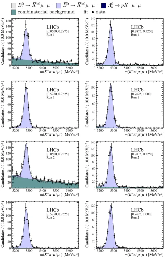
Bs0→ K∗0µ+µ− B0 → K∗0µ+µ− Λ0
b → pK−µ+µ−
combinatorial background − fit • data
5200 5300 5400 5500 5600 ] 2 c ) [MeV/ − µ + µ + π − K ( m 0 20 40 60 80 100 120 140 160 ) 2 c Candidates / ( 10.0 MeV/ LHCb [0.0500, 0.2875] Run 1 5200 5300 5400 5500 5600 ] 2 c ) [MeV/ − µ + µ + π − K ( m 0 20 40 60 80 100 120 140 ) 2 c Candidates / ( 10.0 MeV/ LHCb [0.2875, 0.5250] Run 1 5200 5300 5400 5500 5600 ] 2 c ) [MeV/ − µ + µ + π − K ( m 0 20 40 60 80 100 ) 2 c Candidates / ( 10.0 MeV/ LHCb [0.5250, 0.7625] Run 1 5200 5300 5400 5500 5600 ] 2 c ) [MeV/ − µ + µ + π − K ( m 0 20 40 60 80 100 ) 2 c Candidates / ( 10.0 MeV/ LHCb [0.7625, 1.000] Run 1 5200 5300 5400 5500 5600 ] 2 c ) [MeV/ − µ + µ + π − K ( m 0 20 40 60 80 100 120 140 160 ) 2 c Candidates / ( 10.0 MeV/ LHCb [0.0500, 0.2875] Run 2 5200 5300 5400 5500 5600 ] 2 c ) [MeV/ − µ + µ + π − K ( m 0 20 40 60 80 100 120 140 ) 2 c Candidates / ( 10.0 MeV/ LHCb [0.2875, 0.5250] Run 2 5200 5300 5400 5500 5600 ] 2 c ) [MeV/ − µ + µ + π − K ( m 0 20 40 60 80 100 120 140 ) 2 c Candidates / ( 10.0 MeV/ LHCb [0.5250, 0.7625] Run 2 5200 5300 5400 5500 5600 ] 2 c ) [MeV/ − µ + µ + π − K ( m 0 20 40 60 80 100 120 ) 2 c Candidates / ( 10.0 MeV/ LHCb [0.7625, 1.000] Run 2
Figure 5: Distribution of reconstructed K−π+µ+µ− invariant mass of candidates outside of the
J/ψ and ψ(2S) mass regions in (top four figures) the Run 1 and (bottom four figures) Run 2 data sets. The candidates are divided into four independent bins of increasing neural network response per data taking period.
Bs0 → J/ψ K∗0 B0→ J/ψ K∗0 B0 → K∗0µ+µ− Λ0
b → J/ψ pK−
B+→ J/ψ K+ combinatorial background − fit • data
5200 5300 5400 5500 5600 ] 2 c ) [MeV/ + π − K ψ J/ ( m 1 − 10 1 10 2 10 3 10 ) 2 c Candidates / ( 2.5 MeV/ LHCb [0.0500, 0.2875] Run 1 5200 5300 5400 5500 5600 ] 2 c ) [MeV/ + π − K ψ J/ ( m 1 − 10 1 10 2 10 3 10 ) 2 c Candidates / ( 2.5 MeV/ LHCb [0.2875, 0.5250] Run 1 5200 5300 5400 5500 5600 ] 2 c ) [MeV/ + π − K ψ J/ ( m 1 − 10 1 10 2 10 3 10 ) 2 c Candidates / ( 2.5 MeV/ LHCb [0.5250, 0.7625] Run 1 5200 5300 5400 5500 5600 ] 2 c ) [MeV/ + π − K ψ J/ ( m 1 − 10 1 10 2 10 3 10 4 10 ) 2 c Candidates / ( 2.5 MeV/ LHCb [0.7625, 1.000] Run 1 5200 5300 5400 5500 5600 ] 2 c ) [MeV/ + π − K ψ J/ ( m 1 − 10 1 10 2 10 3 10 4 10 ) 2 c Candidates / ( 2.5 MeV/ LHCb [0.0500, 0.2875] Run 2 5200 5300 5400 5500 5600 ] 2 c ) [MeV/ + π − K ψ J/ ( m 1 − 10 1 10 2 10 3 10 4 10 ) 2 c Candidates / ( 2.5 MeV/ LHCb [0.2875, 0.5250] Run 2 5200 5300 5400 5500 5600 ] 2 c ) [MeV/ + π − K ψ J/ ( m 1 − 10 1 10 2 10 3 10 4 10 ) 2 c Candidates / ( 2.5 MeV/ LHCb [0.5250, 0.7625] Run 2 5200 5300 5400 5500 5600 ] 2 c ) [MeV/ + π − K ψ J/ ( m 1 − 10 1 10 2 10 3 10 4 10 ) 2 c Candidates / ( 2.5 MeV/ LHCb [0.7625, 1.000] Run 2
Figure 6: Distribution of reconstructed J/ψ K−π+ invariant mass after application of a J/ψ
mass constraint of candidates in (top four figures) the Run 1 and (bottom four figures) Run 2 data sets. The candidates are divided into four independent bins of increasing neural network response per data taking period.
References
[1] T. M. Aliev and M. Savci, Exclusive B → π`+`− and B → ρ`+`− decays in two Higgs
doublet model, Phys. Rev. D60 (1999) 014005, arXiv:hep-ph/9812272.
[2] J.-J. Wang, R.-M. Wang, Y.-G. Xu, and Y.-D. Yang, The rare decays B+ →
π+`+`−, ρ+`+`− and B0 → `+`− in the R-parity violating supersymmetry, Phys.
Rev. D77 (2008) 014017, arXiv:0711.0321.
[3] A. Bharucha, D. M. Straub, and R. Zwicky, B → V `+`− in the Standard Model from
light-cone sum rules, JHEP 08 (2016) 098, arXiv:1503.05534.
[4] P. Ball and R. Zwicky, Bd,s → ρ, ω, K∗, φ decay form-factors from light-cone sum
rules revisited, Phys. Rev. D71 (2005) 014029, arXiv:hep-ph/0412079.
[5] R. R. Horgan, Z. Liu, S. Meinel, and M. Wingate, Rare B decays using lattice QCD form factors, PoS LATTICE2014 (2015) 372, arXiv:1501.00367.
[6] Y.-L. Wu, M. Zhong, and Y.-B. Zuo, B(s), D(s) → π, K, η, ρ, K∗, ω, φ transition
form factors and decay rates with extraction of the CKM parameters |Vub|, |Vcs|, |Vcd|,
Int. J. Mod. Phys. A21 (2006) 6125, arXiv:hep-ph/0604007.
[7] R. N. Faustov and V. O. Galkin, Rare Bs decays in the relativistic quark model, Eur.
Phys. J. C73 (2013) 2593, arXiv:1309.2160.
[8] B. Kindra and N. Mahajan, Predictions of angular observables for ¯Bs → K∗`` and
¯
B → ρ`` in Standard Model, arXiv:1803.05876.
[9] LHCb collaboration, R. Aaij et al., First measurement of the differential branching fraction and CP asymmetry of the B+ → π+µ+µ− decay, JHEP 10 (2015) 034,
arXiv:1509.00414.
[10] LHCb collaboration, R. Aaij et al., Observation of the suppressed decay Λ0
b →
pπ−µ+µ−, JHEP 04 (2017) 029, arXiv:1701.08705.
[11] LHCb collaboration, R. Aaij et al., Study of the rare Bs0 and B0 decays into the π+π−µ+µ− final state, Phys. Lett. B743 (2015) 46, arXiv:1412.6433.
[12] D. Du et al., Phenomenology of semileptonic B-meson decays with form factors from lattice QCD, Phys. Rev. D93 (2016) 034005, arXiv:1510.02349.
[13] T. Blake, T. Gershon, and G. Hiller, Rare b hadron decays at the LHC, Ann. Rev. Nucl. Part. Sci. 65 (2015) 113, arXiv:1501.03309.
[14] Belle collaboration, J.-T. Wei et al., Measurement of the differential branching fraction and forward-backward asymmetry for B → K(∗)`+`−, Phys. Rev. Lett. 103 (2009)
171801, arXiv:0904.0770.
[15] BaBar collaboration, J. P. Lees et al., Measurement of branching fractions and rate asymmetries in the rare decays B → K(∗)`+`−, Phys. Rev. D86 (2012) 032012,
[16] CDF collaboration, T. Aaltonen et al., Measurement of the forward-backward asym-metry in the B → K(∗)µ+µ− decay and first observation of the B0
s → φµ+µ
− decay,
Phys. Rev. Lett. 106 (2011) 161801, arXiv:1101.1028.
[17] CMS collaboration, V. Khachatryan et al., Angular analysis of the decay B0 →
K∗0µ+µ− from pp collisions at √s = 8 TeV , Phys. Lett. B753 (2016) 424,
arXiv:1507.08126.
[18] LHCb collaboration, R. Aaij et al., Angular analysis of the B0 → K∗0µ+µ− decay
using 3 fb−1 of integrated luminosity, JHEP 02 (2016) 104, arXiv:1512.04442.
[19] LHCb collaboration, R. Aaij et al., Measurement of the S-wave fraction in B0 → K+π−µ+µ− decays and the B0 → K∗(892)0µ+µ− differential branching fraction,
JHEP 11 (2016) 047, Erratum ibid. 04 (2017) 142, arXiv:1606.04731.
[20] W. Altmannshofer, C. Niehoff, P. Stangl, and D. M. Straub, Status of the B → K∗µ+µ− anomaly after Moriond 2017, Eur. Phys. J. C77 (2017) 377,
arXiv:1703.09189.
[21] M. Ciuchini et al., On flavourful easter eggs for new physics hunger and lepton flavour universality violation, Eur. Phys. J. C77 (2017) 688, arXiv:1704.05447.
[22] V. G. Chobanova et al., Large hadronic power corrections or new physics in the rare decay B → K∗0µ+µ−?, JHEP 07 (2017) 025, arXiv:1702.02234.
[23] L.-S. Geng et al., Towards the discovery of new physics with lepton-universality ratios of b → s`` decays, Phys. Rev. D96 (2017) 093006, arXiv:1704.05446.
[24] B. Capdevila et al., Patterns of new physics in b → s`+`− transitions in the light of
recent data, JHEP 01 (2018) 093, arXiv:1704.05340.
[25] LHCb collaboration, A. A. Alves Jr. et al., The LHCb detector at the LHC, JINST 3 (2008) S08005.
[26] LHCb collaboration, R. Aaij et al., LHCb detector performance, Int. J. Mod. Phys. A30 (2015) 1530022, arXiv:1412.6352.
[27] R. Aaij et al., Performance of the LHCb Vertex Locator, JINST 9 (2014) P09007, arXiv:1405.7808.
[28] R. Arink et al., Performance of the LHCb Outer Tracker, JINST 9 (2014) P01002, arXiv:1311.3893.
[29] M. Adinolfi et al., Performance of the LHCb RICH detector at the LHC, Eur. Phys. J. C73 (2013) 2431, arXiv:1211.6759.
[30] A. A. Alves Jr. et al., Performance of the LHCb muon system, JINST 8 (2013) P02022, arXiv:1211.1346.
[31] R. Aaij et al., The LHCb trigger and its performance in 2011, JINST 8 (2013) P04022, arXiv:1211.3055.
[32] V. V. Gligorov and M. Williams, Efficient, reliable and fast high-level triggering using a bonsai boosted decision tree, JINST 8 (2013) P02013, arXiv:1210.6861.
[33] T. Sj¨ostrand, S. Mrenna, and P. Skands, A brief introduction to PYTHIA 8.1, Comput. Phys. Commun. 178 (2008) 852, arXiv:0710.3820.
[34] I. Belyaev et al., Handling of the generation of primary events in Gauss, the LHCb simulation framework, J. Phys. Conf. Ser. 331 (2011) 032047.
[35] D. J. Lange, The EvtGen particle decay simulation package, Nucl. Instrum. Meth. A462 (2001) 152.
[36] P. Golonka and Z. Was, PHOTOS Monte Carlo: A precision tool for QED corrections in Z and W decays, Eur. Phys. J. C45 (2006) 97, arXiv:hep-ph/0506026.
[37] Geant4 collaboration, J. Allison et al., Geant4 developments and applications, IEEE Trans. Nucl. Sci. 53 (2006) 270; Geant4 collaboration, S. Agostinelli et al., Geant4: A simulation toolkit, Nucl. Instrum. Meth. A506 (2003) 250.
[38] M. Clemencic et al., The LHCb simulation application, Gauss: Design, evolution and experience, J. Phys. Conf. Ser. 331 (2011) 032023.
[39] Particle Data Group, C. Patrignani et al., Review of particle physics, Chin. Phys. C40 (2016) 100001, and 2017 update.
[40] W. D. Hulsbergen, Decay chain fitting with a Kalman filter, Nucl. Instrum. Meth. A552 (2005) 566, arXiv:physics/0503191.
[41] M. Feindt and U. Kerzel, The NeuroBayes neural network package, Nucl. Instrum. Meth. A559 (2006) 190.
[42] LHCb collaboration, R. Aaij et al., Measurement of b-hadron masses, Phys. Lett. B708 (2012) 241, arXiv:1112.4896.
[43] LHCb collaboration, R. Aaij et al., Measurement of the polarization amplitudes in B0 → J/ψ K∗(892)0 decays, Phys. Rev. D88 (2013) 052002, arXiv:1307.2782.
[44] LHCb collaboration, R. Aaij et al., Measurement of the fragmentation fraction ratio fs/fd and its dependence on B meson kinematics, JHEP 04 (2013) 001,
arXiv:1301.5286, fs/fd value updated in LHCb-CONF-2013-011.
[45] LHCb collaboration, R. Aaij et al., Measurement of the B0
s → µ+µ
− branching
fraction and effective lifetime and search for B0 → µ+µ− decays, Phys. Rev. Lett.
118 (2017) 191801, arXiv:1703.05747.
[46] Belle collaboration, K. Chilikin et al., Observation of a new charged charmonium like state in B0 → J/ψ K−π+ decays, Phys. Rev. D90 (2014) 112009, arXiv:1408.6457.
[47] LHCb collaboration, R. Aaij et al., Measurement of CP violation parameters and polar-isation fractions in B0
s → J/ψ K
∗0 decays, JHEP 11 (2015) 082, arXiv:1509.00400.
[48] LHCb collaboration, Framework TDR for the LHCb Upgrade: Technical Design Report, CERN-LHCC-2012-007. LHCb-TDR-012.
LHCb collaboration
R. Aaij43, B. Adeva39, M. Adinolfi48, Z. Ajaltouni5, S. Akar59, P. Albicocco19, J. Albrecht10,
F. Alessio40, M. Alexander53, A. Alfonso Albero38, S. Ali43, G. Alkhazov31,
P. Alvarez Cartelle55, A.A. Alves Jr59, S. Amato2, S. Amerio23, Y. Amhis7, L. An3,
L. Anderlini18, G. Andreassi41, M. Andreotti17,g, J.E. Andrews60, R.B. Appleby56, F. Archilli43,
P. d’Argent12, J. Arnau Romeu6, A. Artamonov37, M. Artuso61, E. Aslanides6, M. Atzeni42,
G. Auriemma26, S. Bachmann12, J.J. Back50, S. Baker55, V. Balagura7,b, W. Baldini17,
A. Baranov35, R.J. Barlow56, S. Barsuk7, W. Barter56, F. Baryshnikov32, V. Batozskaya29,
V. Battista41, A. Bay41, J. Beddow53, F. Bedeschi24, I. Bediaga1, A. Beiter61, L.J. Bel43,
N. Beliy63, V. Bellee41, N. Belloli21,i, K. Belous37, I. Belyaev32,40, E. Ben-Haim8,
G. Bencivenni19, S. Benson43, S. Beranek9, A. Berezhnoy33, R. Bernet42, D. Berninghoff12,
E. Bertholet8, A. Bertolin23, C. Betancourt42, F. Betti15,40, M.O. Bettler49, M. van Beuzekom43,
Ia. Bezshyiko42, S. Bifani47, P. Billoir8, A. Birnkraut10, A. Bizzeti18,u, M. Bjørn57, T. Blake50,
F. Blanc41, S. Blusk61, V. Bocci26, O. Boente Garcia39, T. Boettcher58, A. Bondar36,w,
N. Bondar31, S. Borghi56,40, M. Borisyak35, M. Borsato39,40, F. Bossu7, M. Boubdir9,
T.J.V. Bowcock54, E. Bowen42, C. Bozzi17,40, S. Braun12, M. Brodski40, J. Brodzicka27,
D. Brundu16, E. Buchanan48, C. Burr56, A. Bursche16, J. Buytaert40, W. Byczynski40,
S. Cadeddu16, H. Cai64, R. Calabrese17,g, R. Calladine47, M. Calvi21,i, M. Calvo Gomez38,m,
A. Camboni38,m, P. Campana19, D.H. Campora Perez40, L. Capriotti56, A. Carbone15,e,
G. Carboni25, R. Cardinale20,h, A. Cardini16, P. Carniti21,i, L. Carson52, K. Carvalho Akiba2,
G. Casse54, L. Cassina21, M. Cattaneo40, G. Cavallero20,h, R. Cenci24,p, D. Chamont7,
M.G. Chapman48, M. Charles8, Ph. Charpentier40, G. Chatzikonstantinidis47, M. Chefdeville4,
S. Chen16, S.-G. Chitic40, V. Chobanova39, M. Chrzaszcz40, A. Chubykin31, P. Ciambrone19,
X. Cid Vidal39, G. Ciezarek40, P.E.L. Clarke52, M. Clemencic40, H.V. Cliff49, J. Closier40,
V. Coco40, J. Cogan6, E. Cogneras5, V. Cogoni16,f, L. Cojocariu30, P. Collins40, T. Colombo40,
A. Comerma-Montells12, A. Contu16, G. Coombs40, S. Coquereau38, G. Corti40, M. Corvo17,g,
C.M. Costa Sobral50, B. Couturier40, G.A. Cowan52, D.C. Craik58, A. Crocombe50,
M. Cruz Torres1, R. Currie52, C. D’Ambrosio40, F. Da Cunha Marinho2, C.L. Da Silva73,
E. Dall’Occo43, J. Dalseno48, A. Danilina32, A. Davis3, O. De Aguiar Francisco40,
K. De Bruyn40, S. De Capua56, M. De Cian41, J.M. De Miranda1, L. De Paula2,
M. De Serio14,d, P. De Simone19, C.T. Dean53, D. Decamp4, L. Del Buono8, B. Delaney49,
H.-P. Dembinski11, M. Demmer10, A. Dendek28, D. Derkach35, O. Deschamps5, F. Dettori54,
B. Dey65, A. Di Canto40, P. Di Nezza19, S. Didenko69, H. Dijkstra40, F. Dordei40, M. Dorigo40,
A. Dosil Su´arez39, L. Douglas53, A. Dovbnya45, K. Dreimanis54, L. Dufour43, G. Dujany8,
P. Durante40, J.M. Durham73, D. Dutta56, R. Dzhelyadin37, M. Dziewiecki12, A. Dziurda40,
A. Dzyuba31, S. Easo51, U. Egede55, V. Egorychev32, S. Eidelman36,w, S. Eisenhardt52,
U. Eitschberger10, R. Ekelhof10, L. Eklund53, S. Ely61, A. Ene30, S. Escher9, S. Esen12,
H.M. Evans49, T. Evans57, A. Falabella15, N. Farley47, S. Farry54, D. Fazzini21,40,i, L. Federici25,
G. Fernandez38, P. Fernandez Declara40, A. Fernandez Prieto39, F. Ferrari15, L. Ferreira Lopes41,
F. Ferreira Rodrigues2, M. Ferro-Luzzi40, S. Filippov34, R.A. Fini14, M. Fiorini17,g, M. Firlej28,
C. Fitzpatrick41, T. Fiutowski28, F. Fleuret7,b, M. Fontana16,40, F. Fontanelli20,h, R. Forty40,
V. Franco Lima54, M. Frank40, C. Frei40, J. Fu22,q, W. Funk40, C. F¨arber40, E. Gabriel52,
A. Gallas Torreira39, D. Galli15,e, S. Gallorini23, S. Gambetta52, M. Gandelman2, P. Gandini22,
Y. Gao3, L.M. Garcia Martin71, B. Garcia Plana39, J. Garc´ıa Pardi˜nas42, J. Garra Tico49,
L. Garrido38, D. Gascon38, C. Gaspar40, L. Gavardi10, G. Gazzoni5, D. Gerick12,
E. Gersabeck56, M. Gersabeck56, T. Gershon50, Ph. Ghez4, S. Gian`ı41, V. Gibson49,
O.G. Girard41, L. Giubega30, K. Gizdov52, V.V. Gligorov8, D. Golubkov32, A. Golutvin55,69,
A. Gomes1,a, I.V. Gorelov33, C. Gotti21,i, E. Govorkova43, J.P. Grabowski12, R. Graciani Diaz38,
P. Griffith16, L. Grillo56, L. Gruber40, B.R. Gruberg Cazon57, O. Gr¨unberg67, E. Gushchin34,
Yu. Guz37,40, T. Gys40, C. G¨obel62, T. Hadavizadeh57, C. Hadjivasiliou5, G. Haefeli41,
C. Haen40, S.C. Haines49, B. Hamilton60, X. Han12, T.H. Hancock57, S. Hansmann-Menzemer12,
N. Harnew57, S.T. Harnew48, C. Hasse40, M. Hatch40, J. He63, M. Hecker55, K. Heinicke10,
A. Heister9, K. Hennessy54, L. Henry71, E. van Herwijnen40, M. Heß67, A. Hicheur2, D. Hill57,
P.H. Hopchev41, W. Hu65, W. Huang63, Z.C. Huard59, W. Hulsbergen43, T. Humair55,
M. Hushchyn35, D. Hutchcroft54, P. Ibis10, M. Idzik28, P. Ilten47, K. Ivshin31, R. Jacobsson40,
J. Jalocha57, E. Jans43, A. Jawahery60, F. Jiang3, M. John57, D. Johnson40, C.R. Jones49,
C. Joram40, B. Jost40, N. Jurik57, S. Kandybei45, M. Karacson40, J.M. Kariuki48, S. Karodia53,
N. Kazeev35, M. Kecke12, F. Keizer49, M. Kelsey61, M. Kenzie49, T. Ketel44, E. Khairullin35,
B. Khanji12, C. Khurewathanakul41, K.E. Kim61, T. Kirn9, S. Klaver19, K. Klimaszewski29,
T. Klimkovich11, S. Koliiev46, M. Kolpin12, R. Kopecna12, P. Koppenburg43, S. Kotriakhova31,
M. Kozeiha5, L. Kravchuk34, M. Kreps50, F. Kress55, P. Krokovny36,w, W. Krupa28,
W. Krzemien29, W. Kucewicz27,l, M. Kucharczyk27, V. Kudryavtsev36,w, A.K. Kuonen41,
T. Kvaratskheliya32,40, D. Lacarrere40, G. Lafferty56, A. Lai16, G. Lanfranchi19,
C. Langenbruch9, T. Latham50, C. Lazzeroni47, R. Le Gac6, A. Leflat33,40, J. Lefran¸cois7,
R. Lef`evre5, F. Lemaitre40, O. Leroy6, T. Lesiak27, B. Leverington12, P.-R. Li63, T. Li3, Z. Li61,
X. Liang61, T. Likhomanenko68, R. Lindner40, F. Lionetto42, V. Lisovskyi7, X. Liu3, D. Loh50,
A. Loi16, I. Longstaff53, J.H. Lopes2, D. Lucchesi23,o, M. Lucio Martinez39, A. Lupato23,
E. Luppi17,g, O. Lupton40, A. Lusiani24, X. Lyu63, F. Machefert7, F. Maciuc30, V. Macko41,
P. Mackowiak10, S. Maddrell-Mander48, O. Maev31,40, K. Maguire56, D. Maisuzenko31,
M.W. Majewski28, S. Malde57, B. Malecki27, A. Malinin68, T. Maltsev36,w, G. Manca16,f,
G. Mancinelli6, D. Marangotto22,q, J. Maratas5,v, J.F. Marchand4, U. Marconi15,
C. Marin Benito38, M. Marinangeli41, P. Marino41, J. Marks12, G. Martellotti26, M. Martin6,
M. Martinelli41, D. Martinez Santos39, F. Martinez Vidal71, A. Massafferri1, R. Matev40,
A. Mathad50, Z. Mathe40, C. Matteuzzi21, A. Mauri42, E. Maurice7,b, B. Maurin41,
A. Mazurov47, M. McCann55,40, A. McNab56, R. McNulty13, J.V. Mead54, B. Meadows59,
C. Meaux6, F. Meier10, N. Meinert67, D. Melnychuk29, M. Merk43, A. Merli22,q, E. Michielin23,
D.A. Milanes66, E. Millard50, M.-N. Minard4, L. Minzoni17,g, D.S. Mitzel12, A. Mogini8,
J. Molina Rodriguez1,y, T. Momb¨acher10, I.A. Monroy66, S. Monteil5, M. Morandin23,
G. Morello19, M.J. Morello24,t, O. Morgunova68, J. Moron28, A.B. Morris6, R. Mountain61,
F. Muheim52, M. Mulder43, D. M¨uller40, J. M¨uller10, K. M¨uller42, V. M¨uller10, P. Naik48,
T. Nakada41, R. Nandakumar51, A. Nandi57, I. Nasteva2, M. Needham52, N. Neri22,
S. Neubert12, N. Neufeld40, M. Neuner12, T.D. Nguyen41, C. Nguyen-Mau41,n, S. Nieswand9,
R. Niet10, N. Nikitin33, A. Nogay68, D.P. O’Hanlon15, A. Oblakowska-Mucha28, V. Obraztsov37,
S. Ogilvy19, R. Oldeman16,f, C.J.G. Onderwater72, A. Ossowska27, J.M. Otalora Goicochea2,
P. Owen42, A. Oyanguren71, P.R. Pais41, A. Palano14, M. Palutan19,40, G. Panshin70,
A. Papanestis51, M. Pappagallo52, L.L. Pappalardo17,g, W. Parker60, C. Parkes56,
G. Passaleva18,40, A. Pastore14, M. Patel55, C. Patrignani15,e, A. Pearce40, A. Pellegrino43,
G. Penso26, M. Pepe Altarelli40, S. Perazzini40, D. Pereima32, P. Perret5, L. Pescatore41,
K. Petridis48, A. Petrolini20,h, A. Petrov68, M. Petruzzo22,q, B. Pietrzyk4, G. Pietrzyk41,
M. Pikies27, D. Pinci26, F. Pisani40, A. Pistone20,h, A. Piucci12, V. Placinta30, S. Playfer52,
M. Plo Casasus39, F. Polci8, M. Poli Lener19, A. Poluektov50, N. Polukhina69, I. Polyakov61,
E. Polycarpo2, G.J. Pomery48, S. Ponce40, A. Popov37, D. Popov11,40, S. Poslavskii37,
C. Potterat2, E. Price48, J. Prisciandaro39, C. Prouve48, V. Pugatch46, A. Puig Navarro42,
H. Pullen57, G. Punzi24,p, W. Qian63, J. Qin63, R. Quagliani8, B. Quintana5, B. Rachwal28,
J.H. Rademacker48, M. Rama24, M. Ramos Pernas39, M.S. Rangel2, I. Raniuk45,†,
F. Ratnikov35,x, G. Raven44, M. Ravonel Salzgeber40, M. Reboud4, F. Redi41, S. Reichert10,
A.C. dos Reis1, C. Remon Alepuz71, V. Renaudin7, S. Ricciardi51, S. Richards48, K. Rinnert54,
A. Rogozhnikov35, S. Roiser40, A. Rollings57, V. Romanovskiy37, A. Romero Vidal39,40,
M. Rotondo19, M.S. Rudolph61, T. Ruf40, J. Ruiz Vidal71, J.J. Saborido Silva39, N. Sagidova31,
B. Saitta16,f, V. Salustino Guimaraes62, C. Sanchez Mayordomo71, B. Sanmartin Sedes39,
R. Santacesaria26, C. Santamarina Rios39, M. Santimaria19, E. Santovetti25,j, G. Sarpis56,
A. Sarti19,k, C. Satriano26,s, A. Satta25, D.M. Saunders48, D. Savrina32,33, S. Schael9,
M. Schellenberg10, M. Schiller53, H. Schindler40, M. Schmelling11, T. Schmelzer10, B. Schmidt40,
O. Schneider41, A. Schopper40, H.F. Schreiner59, M. Schubiger41, M.H. Schune7,40,
R. Schwemmer40, B. Sciascia19, A. Sciubba26,k, A. Semennikov32, E.S. Sepulveda8, A. Sergi47,40,
N. Serra42, J. Serrano6, L. Sestini23, P. Seyfert40, M. Shapkin37, Y. Shcheglov31,†, T. Shears54,
L. Shekhtman36,w, V. Shevchenko68, B.G. Siddi17, R. Silva Coutinho42, L. Silva de Oliveira2,
G. Simi23,o, S. Simone14,d, N. Skidmore12, T. Skwarnicki61, I.T. Smith52, M. Smith55,
l. Soares Lavra1, M.D. Sokoloff59, F.J.P. Soler53, B. Souza De Paula2, B. Spaan10, P. Spradlin53,
F. Stagni40, M. Stahl12, S. Stahl40, P. Stefko41, S. Stefkova55, O. Steinkamp42, S. Stemmle12,
O. Stenyakin37, M. Stepanova31, H. Stevens10, S. Stone61, B. Storaci42, S. Stracka24,p,
M.E. Stramaglia41, M. Straticiuc30, U. Straumann42, S. Strokov70, J. Sun3, L. Sun64,
K. Swientek28, V. Syropoulos44, T. Szumlak28, M. Szymanski63, S. T’Jampens4, Z. Tang3,
A. Tayduganov6, T. Tekampe10, G. Tellarini17, F. Teubert40, E. Thomas40, J. van Tilburg43,
M.J. Tilley55, V. Tisserand5, M. Tobin41, S. Tolk40, L. Tomassetti17,g, D. Tonelli24,
R. Tourinho Jadallah Aoude1, E. Tournefier4, M. Traill53, M.T. Tran41, M. Tresch42,
A. Trisovic49, A. Tsaregorodtsev6, A. Tully49, N. Tuning43,40, A. Ukleja29, A. Usachov7,
A. Ustyuzhanin35, U. Uwer12, C. Vacca16,f, A. Vagner70, V. Vagnoni15, A. Valassi40, S. Valat40,
G. Valenti15, R. Vazquez Gomez40, P. Vazquez Regueiro39, S. Vecchi17, M. van Veghel43,
J.J. Velthuis48, M. Veltri18,r, G. Veneziano57, A. Venkateswaran61, T.A. Verlage9, M. Vernet5,
M. Vesterinen57, J.V. Viana Barbosa40, D. Vieira63, M. Vieites Diaz39, H. Viemann67,
X. Vilasis-Cardona38,m, A. Vitkovskiy43, M. Vitti49, V. Volkov33, A. Vollhardt42, B. Voneki40,
A. Vorobyev31, V. Vorobyev36,w, C. Voß9, J.A. de Vries43, C. V´azquez Sierra43, R. Waldi67,
J. Walsh24, J. Wang61, M. Wang3, Y. Wang65, Z. Wang42, D.R. Ward49, H.M. Wark54,
N.K. Watson47, D. Websdale55, A. Weiden42, C. Weisser58, M. Whitehead9, J. Wicht50,
G. Wilkinson57, M. Wilkinson61, M.R.J. Williams56, M. Williams58, T. Williams47,
F.F. Wilson51,40, J. Wimberley60, M. Winn7, J. Wishahi10, W. Wislicki29, M. Witek27,
G. Wormser7, S.A. Wotton49, K. Wyllie40, D. Xiao65, Y. Xie65, A. Xu3, M. Xu65, Q. Xu63,
Z. Xu3, Z. Xu4, Z. Yang3, Z. Yang60, Y. Yao61, H. Yin65, J. Yu65, X. Yuan61, O. Yushchenko37,
K.A. Zarebski47, M. Zavertyaev11,c, L. Zhang3, Y. Zhang7, A. Zhelezov12, Y. Zheng63, X. Zhu3,
V. Zhukov9,33, J.B. Zonneveld52, S. Zucchelli15.
1Centro Brasileiro de Pesquisas F´ısicas (CBPF), Rio de Janeiro, Brazil 2Universidade Federal do Rio de Janeiro (UFRJ), Rio de Janeiro, Brazil 3Center for High Energy Physics, Tsinghua University, Beijing, China
4Univ. Grenoble Alpes, Univ. Savoie Mont Blanc, CNRS, IN2P3-LAPP, Annecy, France 5Clermont Universit´e, Universit´e Blaise Pascal, CNRS/IN2P3, LPC, Clermont-Ferrand, France 6Aix Marseille Univ, CNRS/IN2P3, CPPM, Marseille, France
7LAL, Univ. Paris-Sud, CNRS/IN2P3, Universit´e Paris-Saclay, Orsay, France
8LPNHE, Universit´e Pierre et Marie Curie, Universit´e Paris Diderot, CNRS/IN2P3, Paris, France 9I. Physikalisches Institut, RWTH Aachen University, Aachen, Germany
10Fakult¨at Physik, Technische Universit¨at Dortmund, Dortmund, Germany 11Max-Planck-Institut f¨ur Kernphysik (MPIK), Heidelberg, Germany
12Physikalisches Institut, Ruprecht-Karls-Universit¨at Heidelberg, Heidelberg, Germany 13School of Physics, University College Dublin, Dublin, Ireland
14Sezione INFN di Bari, Bari, Italy 15Sezione INFN di Bologna, Bologna, Italy 16Sezione INFN di Cagliari, Cagliari, Italy 17Sezione INFN di Ferrara, Ferrara, Italy
18Sezione INFN di Firenze, Firenze, Italy
19Laboratori Nazionali dell’INFN di Frascati, Frascati, Italy 20Sezione INFN di Genova, Genova, Italy
21Sezione INFN di Milano Bicocca, Milano, Italy 22Sezione INFN di Milano, Milano, Italy
23Sezione INFN di Padova, Padova, Italy 24Sezione INFN di Pisa, Pisa, Italy
25Sezione INFN di Roma Tor Vergata, Roma, Italy 26Sezione INFN di Roma La Sapienza, Roma, Italy
27Henryk Niewodniczanski Institute of Nuclear Physics Polish Academy of Sciences, Krak´ow, Poland 28AGH - University of Science and Technology, Faculty of Physics and Applied Computer Science,
Krak´ow, Poland
29National Center for Nuclear Research (NCBJ), Warsaw, Poland
30Horia Hulubei National Institute of Physics and Nuclear Engineering, Bucharest-Magurele, Romania 31Petersburg Nuclear Physics Institute (PNPI), Gatchina, Russia
32Institute of Theoretical and Experimental Physics (ITEP), Moscow, Russia
33Institute of Nuclear Physics, Moscow State University (SINP MSU), Moscow, Russia
34Institute for Nuclear Research of the Russian Academy of Sciences (INR RAS), Moscow, Russia 35Yandex School of Data Analysis, Moscow, Russia
36Budker Institute of Nuclear Physics (SB RAS), Novosibirsk, Russia 37Institute for High Energy Physics (IHEP), Protvino, Russia
38ICCUB, Universitat de Barcelona, Barcelona, Spain
39Instituto Galego de F´ısica de Altas Enerx´ıas (IGFAE), Universidade de Santiago de Compostela,
Santiago de Compostela, Spain
40European Organization for Nuclear Research (CERN), Geneva, Switzerland
41Institute of Physics, Ecole Polytechnique F´ed´erale de Lausanne (EPFL), Lausanne, Switzerland 42Physik-Institut, Universit¨at Z¨urich, Z¨urich, Switzerland
43Nikhef National Institute for Subatomic Physics, Amsterdam, The Netherlands
44Nikhef National Institute for Subatomic Physics and VU University Amsterdam, Amsterdam, The
Netherlands
45NSC Kharkiv Institute of Physics and Technology (NSC KIPT), Kharkiv, Ukraine
46Institute for Nuclear Research of the National Academy of Sciences (KINR), Kyiv, Ukraine 47University of Birmingham, Birmingham, United Kingdom
48H.H. Wills Physics Laboratory, University of Bristol, Bristol, United Kingdom 49Cavendish Laboratory, University of Cambridge, Cambridge, United Kingdom 50Department of Physics, University of Warwick, Coventry, United Kingdom 51STFC Rutherford Appleton Laboratory, Didcot, United Kingdom
52School of Physics and Astronomy, University of Edinburgh, Edinburgh, United Kingdom 53School of Physics and Astronomy, University of Glasgow, Glasgow, United Kingdom 54Oliver Lodge Laboratory, University of Liverpool, Liverpool, United Kingdom 55Imperial College London, London, United Kingdom
56School of Physics and Astronomy, University of Manchester, Manchester, United Kingdom 57Department of Physics, University of Oxford, Oxford, United Kingdom
58Massachusetts Institute of Technology, Cambridge, MA, United States 59University of Cincinnati, Cincinnati, OH, United States
60University of Maryland, College Park, MD, United States 61Syracuse University, Syracuse, NY, United States
62Pontif´ıcia Universidade Cat´olica do Rio de Janeiro (PUC-Rio), Rio de Janeiro, Brazil, associated to 2 63University of Chinese Academy of Sciences, Beijing, China, associated to3
64School of Physics and Technology, Wuhan University, Wuhan, China, associated to3
65Institute of Particle Physics, Central China Normal University, Wuhan, Hubei, China, associated to3 66Departamento de Fisica , Universidad Nacional de Colombia, Bogota, Colombia, associated to8 67Institut f¨ur Physik, Universit¨at Rostock, Rostock, Germany, associated to 12
68National Research Centre Kurchatov Institute, Moscow, Russia, associated to32
69National University of Science and Technology MISIS, Moscow, Russia, associated to32 70National Research Tomsk Polytechnic University, Tomsk, Russia, associated to 32