Adaptation to a linear vection stimulus in a virtual reality environment

Adaptation to a Linear Vection Stimulus in a Virtual

Reality Environment

by

Christine A. Tovee

Bachelor of Applied Science in Engineering Science with Aerospace Concentration University of Toronto, 1993.

Submitted to the Department of Aeronautics and Astronautics in Partial Fulfillment of the Requirements for the Degree of

Master of Science in Aeronautics and Astronautics

at the

Massachusetts Institute of Technology

February 1999

0 1999 Massachusetts Institute of Technology All rights reserved.

Signature of Author:

Department of Aeronautics and Astronautics February 2, 1999

Certified by:

Dr. Charles M. Oman Director, Man-Vehicle Lab, Senior Lecturer, Dept. of Aeronautics and Astronautics Thesis Supervisor

Accepted by:

Professor Jaime Peraire Chair, Graduate Office

Adaptation to a Linear Vection Stimulus in a Virtual

Reality Environment

by

Christine A. Tovee

Submitted to the Department of Aeronautics and Astronautics on February 2, 1999 in Partial Fulfillment of the Requirements for the Degree of Master of Science in

Aeronautics and Astronautics

Abstract

In the zero-gravity environment of space, the vestibular system's functioning is compromised and astronauts receive conflicting visual and vestibular cues concerning body orientation and motion. Experiment 136 on the Neurolab space shuttle mission

explored this research question. The current experiment served as a supporting study, examining human "looming linear vection" responses produced by a virtual checkerboard hallway scene moving towards the observer. In the Earth's gravity environment, the

input of the vestibular system can be explored by setting the subject's body orientation (and axis of the vestibular system) in line with or perpendicular to the gravity axis. Five different virtual scene speeds were used. Six vection measures were calculated for each trial: latency, decay latency, peak magnitude of perceived self motion, rise time of magnitude, rise slope, and area (integrated distance traveled). In addition, both latency and magnitude of self-motion were examined for signs of adaptation. Particularly at low scene speeds, the latency of the onset of looming vection was significantly greater in the supine than upright posture, opposite to the effect reported by Kano (1991). Most subjects interpreted the scene as a moving horizontal hallway and the conflict between the visual and gravitational verticals may have delayed the onset of vection in the supine posture. Posture did not affect the magnitude values indicating that the vestibular system plays a minimal role in the perception of speed of self-motion. Virtual scene speed influenced all measures significantly except after-latencies. Latency decreased slightly over the first few trials in the upright posture. However, for both latency and magnitude, adaptation to the stimulus seems to be minimal when considering changes over time in either measure.

Thesis Supervisor: Charles M. Oman

Title: Director of Man-Vehicle Lab, Senior Lecturer, Dept. of Aeronautics and Astronautics

Press on:

Nothing in the world can take the place of perseverance. Talent will not;

Nothing is more common than unsuccessful men with talent. Genius will not;

Unrewarded genius is almost a proverb. Education will not;

The world is full of educated derelicts.

Persistence and determination alone are omnipotent. Press on!

Acknowledgements

I would like to thank the following individuals and groups for their assistance during the

making of this thesis:

My family for their enthusiastic support and unyielding faith,

James C. Reardon for being steadfast and thinking my work was important,

Dr. Charles M. Oman for giving me the opportunity to work on the Neurolab project, Dr. Alan Natapoff for his kind words and his assistance with the statistical analysis, Drs. Andy Beall and Ted Carpenter-Smith for their advice and fellowship,

Prof. Richard Held for his insights and suggestions regarding the experimental concept,

All subjects for their participation and their patience,

Members of the Man-Vehicle Lab,

Andjelka Kelic, Matthew Greenman, Edward Piekos, and Matthew Knapp for offering their friendship, their humour and the occasional paddle,

The Lockheed-Martin VEG Team at NASA Johnson Space Center for technical support, Prof. John Deyst for reminding me of the importance of responsibility,

Lynn Roberson, Richard Goldhammer, and Jennifer Knapp-Stomp for convincing me that this work is only the opening overture,

Profs. Dava Newman and John-Paul Clarke, and Elizabeth Zotos.

Partial funding for this work was provided by NASA under contracts: NAS9-19536 and

Table of Contents

JOYSTICK CALIBRATION PROCEDURE 29

TEST PROCEDURE 30 MEASUREMENTS 31 RESULTS 33 CALIBRATION 33 PROFILES 37 SUBJECT VARIABILITY 38 LATENCY 41 MAXIMUM MAGNITUDE 44

AREA UNDER THE CURVE 48

RISE TIME 48 RISE SLOPE 49 ADAPTATION 50 Aftereffects 50 Repetition 53 DISCUSSION 57 MAGNITUDE ESTIMATION 57 USEFULNESS OF CALIBRATION 60 SPEED 62 POSTURE 62 ADAPTATION 64 Vection Aftereffects 64 Repetition 65 FUTURE WORK 65

CONCLUSION

BIBLIOGRAPHY 70

APPENDIX A -SUBJECT QUESTIONNAIRE AND INSTRUCTION SET 72

VIRTUAL ENVIRONMENT QUESTIONNAIRE 72

INSTRUCTIONS FOR SUBJECTS 75

APPENDIX B- COMMITTEE ON THE USE OF HUMANS AS EXPERIMENTAL SUBJECTS

(COUHES) EXPERIMENT DESCRIPTION 77

APPENDIX C- MATLAB DATA ANALYSIS SCRIPTS 79

AFTERRAW.M 79

AFTERRAWTRANS.M 85

MAGANALYZE.M 91

APPENDIX D- EARLY AND LATE REPETITIONS COMPARED 93

APPENDIX E- VECTION MAGNITUDE PROFILES 99

Table of Figures

FIGURE 1- VIRTUAL ENVIRONMENT EQUIPMENT- UPRIGHT POSTURE ... 26

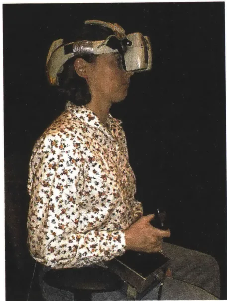
FIGURE 2- SUBJECT IN SUPINE POSTURE ... 27

FIGURE 3-VECTION STIMULUS-VIRTUAL TUNNEL wrTH FRAME ... 29

FIGURE 4-VECTION MEASURES, SIMULATED DATA FOR A SINGLE TRIAL ... 32

FIGURE 5-TYPICAL CALIBRATION DATA (SUBJECT 14)... 33

FIGURE 6- T-TEST VALUES FOR PRFIPOST REGRESSION VARIABLE ... 35

FIGURE 7-INDIVIDuAL CALIBRATION CURVES, INTERCEPT VALUES- THE IDEAL CALIBRATION CURVE HAS AN INTERCEPT EQUAL TO 128. ... 36

FIGURE 8- INDIVIDUAL CALIBRATION CURVES- SLOPE VALUES THE SLOPE OF THE IDEAL CALIBRATION CURVE EQUALS -1.28 ... 36

FIGURE 9- TYPICAL MAGNITUDE PROFILES FOR THE FIRST TWO TRIALS AT SPEED 3 FOR EACH EXPERIMENTAL BLOCK. (RECALL THAT SPEED 3 WAS DESIGNATED THE MODULUS AND THE SUBJECT WAS INSTRUCTED TO DEFLECT THE JOYSTICK 50% TO INDICATE THE MAXIMUM MAGNITUDE OF THAT TRIAL). ... 38

FIGURE 10- PERCENT OF TRIALS ACHIEVING VECTION... 39

FIGURE 11- NUMBER OF TRIALS wrrH VECTION AS A FUNCTION OF POSTURE ... 40

FIGURE 12- NUMBER OF VECTION TRIALS AS A FUNCTION OF PRESENTATION ORDER ... 41

FIGURE 13-LATENCIES VS. SPEED, UPRIGHT POSTURE ... 42

FIGURE 14-LATENCIES VS. SPEED, SUPINE CONDITION ... 43

FIGURE 15- MEAN LATENCIES UPRIGHT AND SUPINE COMPARED ... 43

FIGURE 16- Box PLOT OF MAXIMUM MAGNITUDE DISTRIBUTION VS. SPEED, SUPINE PO STURE ... 44

FIGURE 17- Box PLOT OF MAXIMUM MAGNITUDE DISTRIBUTION VS. SPEED, UPRIGHT PO STU RE ... 45

FIGURE 18- Box PLOT OF TRANSFORMED MAXIMUM MAGNITUDE DISTRIBUTION VS. SPEED, U PRIGHT POSTURE ... 45

FIGURE 19-Box PLOT OF MAXIMUM TRANSFORMED MAGNITUDE DISTRIBUTION V. SPEED-SUPINE POSTURE ... .. 46

FIGURE 20-MAxIMUM MAGNITUDE VS. SPEED, UPRIGHT POSTURE ... 46

FIGURE 21- MAxIMUM MAGNITUDE VS. SPEED, SUPINE POSTURE ... 47

FIGURE 22-MAxIMUM MAGNITUDE, SUPINE AND UPRIGHT COMPARED ... 47

FIGURE 23- MEAN AREA, UPRIGHT AND SUPINE POSTURES COMPARED ... 48

FIGURE 24- MEAN RISE TIME, UPRIGHT AND SUPINE POSTURES COMPARED ... 49

FIGURE 25- MEAN TRANSFORMED SLOPE, UPRIGHT AND SUPINE COMPARED ... 50

FIGURE 26- MEAN DECAY LATENCIES, SUBJECTS REPORTING AFTEREFFECTS (YES GROUP) ARE COMPARED TO SUBJECTS WHO DID NOT (NO GROUP). MEANS FOR BOTH UPRIGHT AND SUPINE POSTURES ARE PLOTTED. ... 51

FIGURE 27- INDIVIDUAL AFTER-LATENCY MEANS FOR SUBJECTS REPORTING AFTEREFFECTS (YES GROUP) AND FOR THOSE NOT REPORTING THEM (NO GROUP)- UPRIGHT POSTURE.52 FIGURE 28 - INDIVIDUAL AFTER-LATENCY MEANS FOR SUBJECTS REPORTING AFTEREFFECTS (YES GROUP) AND FOR THOSE NOT REPORTING THEM (NO GROUP)- SUPINE POSTURE.52 FIGURE 29- MEAN LATENCY VS. REPETITION, SUPINE POSTURE ... 54

FIGURE 30- MEAN LATENCY VS. REPETITION, UPRIGHT POSTURE... 55

FIGURE 31- MEAN MAX. MAGNITUDE VS. REPETITION, SUPINE POSTURE ... 55

FIGURE 32- MEAN MAX. MAGNITUDE VS. REPETITION, UPRIGHT POSTURE ... 56

FIGURE 33- HYPOTHETICAL MAXIMUM MAGNITUDE CURVES- CHANGE IN POSTURE CAUSED A SHIFT IN THE INTERCEPT (CASEl). ... 58

FIGURE 34-HYPOTHETiCAL MAXIMUM MAGNITUDE CURVES- POSTURE PRODUCED A CHANGE IN SLOPE BUT THE PERCEPTION AT THE MODULUS SPEED IS EQUAL IN BOTH CONDITIONS (CASE 2). ... 58

FIGURE 35- HYPOTHETICAL MAXIMUM MAGNITUDE CURVES- POSTURE PRODUCED BOTH A SHIFT AT THE MODULUS SPEED AND A CHANGE IN SLOPE (CASE 3) ... 59

FIGURE 36- MAXIMUM MAGNITUDE- MEANS FOR ALL SUBJECTS CALCULATED FROM INDIVIDUAL CALIBRATION CURVES COMPARED WITH VALUES FROM GENERAL IDEAL CALIBRATION CURVE. ... 61

FIGURE 37- STANDARD ERROR OF THE MEAN FOR MAXIMUM MAGNITUDE, COMPARISON BETWEEN VALUES CALCULATED WITH INDIVIDUAL CALIBRATION CURVES AND VALUES USING IDEAL CALIBRATION CURVE. ... 61

FIGURE 38- LATENCY, UPRIGHT POSTURE ... 93

FIGURE 39- LATENCY, SUPINE POSTURE ... 93

FIGURE 40- MEAN DECAY, UPRIGHT POSTURE ... 94

FIGURE 41- AFTER DECAY- SUPINE POSTURE ... 94

FIGURE 42- MAX. MAGNITUDE, UPRIGHT POSTURE ... 95

FIGURE 43- MAX. MAGNITUDE, SUPINE POSTURE ... 95

FIGURE 44-RISE TIME- UPRIGHT POSTURE ... 96

FIGURE 45- MEAN RISE TIME, SUPINE PoSTURE ... 96

FIGURE 46- MEAN AREA, UPRIGHT POSTURE ... 97

FIGURE 47- AREA- SUPINE POSTURE ... 97

FIGURE 48-SLOPE, UPRIGHT POSTURE ... 98

FIGURE 49- SLOPE, SUPINE POSTURE ... 98

FIGURE 50- SUBJECT 1 PROFILES, UPRIGHT POSTURE ... 99

FIGURE 51- SUBJECT 1 PROFILES, SUPINE POSTURE ... 99

FIGURE 52- SUBJECT 2 PROFILES, UPRIGHT POSTURE ... 100

FIGURE 53-SUBJECT 2 PROFILES, SUPINE POSTURE ... 100

FIGURE 54-SUBJECT 3 PROFILES, UPRIGHT POSTURE ... 101

FIGURE 55- SUBJECT 3 PROFILES, SUPINE POSTURE ... 101

FIGURE 56-SUBJECT 4 PROFILES, UPRIGHT POSTURE ... 102

FIGURE 57- SUBJECT 4 PROFILES, SUPINE POSTURE ... 102

FIGURE 58-SUBJECT 5 PROFILES, UPRIGHT POSTURE ... 103

FIGURE 59- SUBJECT 5 PROFILES, SUPINE POSTURE ... 103

FIGURE 60- SUBJECT 6 PROFILES, UPRIGHT POSTURE ... 104

FIGURE 61- SUBJECT 6 PROFILES, SUPINE POSTURE ... 104

FIGURE 62- SUBJECT 7 PROFILES, UPRIGHT POSTURE ... 105

FIGURE 63- SUBJECT 7 PROFILES - SUPINE POSTURE ... 105

FIGURE 64- SUBJECT 8 PROFILES, UPRIGHT POSTURE ... 106

FIGURE 65-SUBJECT 8 PROFILES, SUPINE POSTURE ... 106

FIGURE 67- SUBJECT 9 PROFILES, SUPINE POSTURE ... 107

FIGURE 68- SUBJECT 10 PROFILES, UPRIGHT POSTURE ... 108

FIGURE 69- SUBJECT 10 PROFILES, SUPINE POSTURE ... 108

FIGURE 70-SUBJECT 12 PROFILES, UPRIGHT POSTURE ... 109

FIGURE 71- SUBJECT 12 PROFILES, SUPINE POSTURE ... 109

FIGURE 72- SUBJECT 13 PROFILES, UPRIGHT POSTURE ... 110

FIGURE 73-SUBJECT 13 PROFILES, SUPINE POSTURE ... 110

FIGURE 74- SUBJECT 14 PROFILES, UPRIGHT POSTURE ... I11 FIGURE 75-SUBJECT 14 PROFILES, SUPINE POSTURE ... 111

List of Tables

TABLE 1 -EXPERIMENT T IM ... E LINE 31 TABLE 2 PRE- AND POST- ExPERiwENT CALIBRATION REGRESSION RESULTS, * =

SIGNIFICANT PREIPOST COEFFICIENT AT P = 0.05... 34 TABLE 3-REGRESSION PARAMETER T-TEST VALUES ... 35

Introduction

Motivation

The visual perception of motion consists of more than the detection of image movement on the retina. Gibson separated the perception of motion into three related problems: object motion, surround stabilization, and observer movement (Gibson, 1954). In the case of observer movement, or self-motion, the visual, vestibular and somatosensory systems interact to detect self-motion. When motion cues from the various senses conflict, the central nervous system (CNS) typically combines them to arrive at a single interpretation by weighing one cue more than another. The sensory conflict created between the visual and modified vestibular systems is thought to contribute to space sickness experienced by astronauts.

Astronauts must detect motion accurately to perform tasks involved in navigation and the manipulation of objects. In space, the Earth's gravitational force no longer provides a reference direction in relation to which body orientation and motion can be defined. Without this reference frame, astronauts sometimes become disoriented and susceptible to space sickness. The visual-vestibular sensory conflict is also a consequence of the use of immersive virtual environments. For many years, astronauts have been using flight simulators with wide field visual displays, and more recently they have trained for extravehicular activities using immersive virtual reality based systems. In the future, virtual reality technology may be used to train for certain other types of activities inside the spacecraft, and to remotely control spacecraft and manipulation systems. In most of these applications, the user interprets scene motion as self motion rather than surround motion, thus experiencing an illusion known as vection.

The term vection was first defined in the 1930's by Fischer and Kornmuller

(Fischer, 1930). When viewing a moving scene, a stationary observer may, after a delay, spontaneously report a sensation of self-motion or vection. Vection may become

Many individuals experience vection in ordinary situations. For instance, a passenger on a train, who, in her peripheral vision, sees another train on the adjacent tracks begin to move, may experience linear vection, a sensation of self-motion in the opposite direction to the movement of the adjacent train. Vection experiments provide an opportunity to investigate the visual and vestibular contributions to the detection of self-motion. It is hypothesized that the latency of the vection onset depends on the relative weighting given to visual versus gravireceptor cues.

Synopsis

This investigation intended to confirm and expand on an earlier investigation by Kano' regarding the influence of the gravitational and visual frames on the latency of linear vection's onset (Kano, 1991). The Kano stimulus was produced by moving patterns displayed in the subject's peripheral vision on large monitors on either side of the subject. The present experiment used a "looming" vection stimulus. Subjects wearing a stereoscopic helmet mounted display (HMD) viewed a virtual checkerboard hallway moving towards them. As in Kano's study, experiments were conducted in both upright and supine postures with several different scene speeds. Six different measures,

including latency and maximum magnitude of perceived speed of self-motion, were analyzed for the influence of scene speed and posture. A speed trend was found for all measures except rise time and after-latency, but only latency and rise time exhibited a change with posture.

In this investigation, the data was examined for signs of two types of adaptation over short time periods. There was no opportunity to explore long-term adaptation. Aftereffects have long been studied as an indication of habituation of motion-sensing processes. This experiment searched for the existence for an analogous aftereffect for

self-motion experienced after the moving stimulus was removed. After each trial, the visual scene was blacked out and the length of time over which vection persisted was recorded. The data offered no conclusive evidence that a vection aftereffect existed.

Secondly, latency and peak magnitude values were examined for changes with repeated exposure to the stimulus. It was hypothesized that subjects would become more

susceptible to vection with repeated trials as mental pathways learned to accept the moving scene as evidence of self-motion. Magnitude results did not exhibit any

adaptation effects over repetition. Upright latencies decreased marginally over the first few repetitions.

This experiment served as a preliminary ground study for a looming vection experiment being conducted during the STS-90 Neurolab Space Shuttle Mission (Experiment 136). It was hypothesized that astronauts would pay less attention to gravireceptor cues and more attention to visual cues after adapting to zero-gravity, and therefore the latency of looming linear vection would decrease in space. Based on Kano's study, it was decided to test astronaut responses to looming linear vection stimuli in both erect and supine postures, preflight and postflight, expecting that spaceflight might affect the difference between erect and supine responses. The present experiments thus served as a control study to verify the effects of posture and scene velocity on a more general population. Therefore, many of the experiment parameters were tailored to apply to the operating constraints of a time intensive mission in space. For example, since a joystick was used to collect all data, calibration protocols were developed to interpret the subject's

responses. Many of the analysis tools developed for this study will be applied to the data from the Neurolab mission.

This paper will discuss the research background in section 2, the experimental design in section 3. The results will be presented in section 4 and then their implications will be discussed in section 5. Future work will be considered in section 6.

Background

Vection

The visual, vestibular and somatosensory systems all provide information about a person's movement. This experiment explores the visual-vestibular interactions in detecting self-motion during vection. The otoliths in a stationary observer will correctly signal a lack of movement (acceleration) but the addition of full scene motion will provide visual cues indicating observer movement. Eventually one interpretation prevails over the other. Vection occurs when the visual cues dominate. Most research has examined circular vection where the subject views a scene rotating around a body aligned axis. For the purposes of this research, scene is defined as the visual perspective encompassing the observer's entire field of view. Linear vection is "elicited by exposing stationary observers to a visual display that expands, contracts, or moves unidirectionally in the frontal or lateral field of view" (Carpenter-Smith, 1995). Looming vection, in response to an expanding optical flow in the frontal plane, was studied because no confounding illusions of pitch or roll are induced. Also, on Neurolab, the vection stimuli was projected using a helmet mounted display (HMD). Because it was not possible to deliver a very wide field of view vection stimuli in the HMD, a looming linear vection stimulus best suited the experimental equipment constraints. The central visual field has been shown to be sensitive to expanding or contracting optical flows and can detect forward/aft self-motion. Experiments have indicated that a small aperture in the central visual field can detect changes of heading (Warren, 1992) and produce compelling looming linear vection.

The strength of vection can also be enhanced by shifting the scene motion into the visual background. Other experiments have achieved this by placing an occluding fixation

surface in front of the display (Kano, 1991). The subject is instructed to focus on the near surface. Howard and Howard used a frame to achieve the same goal in circular

vection experiments (Howard, 1994). They reported a significant increase in vection intensity and a decrease in onset latency due to the presence of the bars in the foreground compared to the no bar condition.

The strength of the observer's vection has also been measured by their perceived speed of self-motion. Some studies examining circularvection have found a correlation between scene velocity and perceived speed of self-motion. However, this finding has been contradicted in other experiments and may only hold for low speeds of rotation. For linear vection induced by a peripheral-vision stimulus, Berthoz, Parvard and Young found that vection magnitude increased with graphic velocity up to approximately 1 m/s and then saturated at this level for all higher speeds (Berthoz, 1975). Kano also reports a link between the perceived speed of self-motion and scene speed (Kano, 1991).

Kano Experiment

The experimental protocol closely imitated Kano's vection experiment (Kano, 1991). The Kano investigation compared the effect of aligning the body/head axis with gravity

(upright posture) to that of setting the axes perpendicular to each other (supine posture). The experimental design also varied stimulus speed and direction of motion within the upright and supine postures. The stimulus consisted of a random dot pattern displayed on two flat screen monitors set opposite each other, on either side of the subject's head, at 90' in the peripheral visual field of the subject. The dots moved across the screen in one of four directions (front, back, up, or, down). The two monitors subtended a total visual angle of approximately 5000 deg2 _{(2x60*x 41.8 1). This angle is more than two} times the size of the HMD's display. Subjects opened their eyes once the moving display reached a constant speed. Three stimulus speeds, 10.5, 25.4, and 41.2 degrees/sec, were presented. At the point of vection onset, the subject pushed a pedal. Each trial lasted twenty seconds. The results demonstrated that latencies for the onset of vection were shorter in the supine posture than in the upright one. The results also depended on the direction of motion within each posture. For forward vection along the body's z-axis, latencies ranged between 2.5 and 4.3 seconds in the former posture and 8 to 10 seconds

in the latter. A speed effect was also detected with latencies decreasing with increasing speed for both postures. Subjects also reported a shift in the perceived speed of self-motion. The effect was categorized (low, medium, or high) but not quantified. Three trials per speed, per direction were presented to each subject. The small number of trials limited the experiment's ability to estimate between subject variability. No training is mentioned as part of the procedure.

The reduction in vection latencies due to posture supports the hypothesis that the

vestibular system plays a role in vection. It appears that the delay in the onset of vection is necessary to overcome the antagonistic input of the vestibular system which signals that the subject is not moving. The vestibular system consists of the three semicircular canals and the two otoliths named the utricular and saccule maculae. The semicircular canals detect angular acceleration and their functioning is not relevant to this discussion. The otoliths are designed to detect linear accelerations and the direction of gravity. When motion is initiated, the maculae's ciliae are deflected by the body's acceleration and the otoliths send a signal to the brainstem. Once the body's motion reaches a constant velocity, the otolith signal decays according to a physiologically determined time constant and only visual cues indicate that the subject is actually in motion. It is hypothesized that the initial lack of vestibular cues to corroborate the interpretation of scene motion as observer movement causes the latency of the onset of vection. The subject eventually experiences vection because after a time the brainstem no longer expects any vestibular cues because of constant velocity motion and the visual cues

dominate the brain's interpretation of body motion. In the supine posture, the otoliths are deflected by gravity in a direction analogous to an acceleration along the body's z-axis and therefore the vection latency should be reduced because the visual and vestibular cues both correspond to body motion along the x-axis.

Magnitude Estimation

Psychophysics attempts to relate the size of human responses to the size of the stimulus. In essence, the goal is to "measure the strength of an experience". S. S. Stevens

developed the technique of magnitude estimation for this purpose. Many perceptions such as loudness, temperature and brightness follow a power law of the form,

XV---KV, ₍₁₎

between a physical stimulus (4), such as amplitude of a sound wave and its related perception, (W), such as loudness where r is the constant of proportionality and 0 is the

exponent (Stevens, 1974). The power law can be restated in the form "equal stimulus ratios produce equal sensation ratios". This ratio invariance applies to all the sensory

systems investigated up to this time.

Magnitude estimation assigns numbers to perceptions proportional to their apparent strength. Alternatively, cross modal sensation matching can be used to estimate the sensation ratios and has also been shown to be reliable. The loudness scale has been used to characterize the scale of a variety of perceptions such as taste and angular velocity and thermal discomfort. For example, a subject could measure the sweetness of a selection of foods by assigning an equivalent loudness of a sound source or the intensity of the

sensation can be graded by the length of a bar on a computer screen. If the physical stimuli,

4,

according to Eq. (1), then sensation matching requires choosing W1=I 2and so

C=4A)r 12 ", where p12 =p2/pi1. (2)

Therefore, for sensation matching, the ratio scale has an exponent,

P,

scale was anchored at the midpoint rather than the endpoints. Subjects were instructed to treat the vection magnitude ratio of the modulus as equal to 50% of the joystick

Other methods to measure the strength of vection have been developed. Some

experiments have measured postural sway in response to a sinusoidal linear motion. This paradigm tests responses to acceleration cues rather than to a constant velocity condition. Another method involves the use of a nulling paradigm where the subject must try to

control the motion of the cart they are riding while viewing a moving visual scene

(Carpenter-Smith, 1995). The shift in the point of subjective equality (PSE) indicates the strength of the vection. Both these alternatives require large set-ups that would not be possible on the space shuttle. Secondly, neither method allows for the examination of the

development of vection in a single trial. Magnitude estimation with the joystick

deflection allows the subject to continuously report the speed of perceived vection during a trial.

Adaptation

Passengers in motor vehicles have difficulty accurately estimating their speed especially after long periods of travel at high velocities (Denton, 1966). In their extensive study of linear vection, Berthoz, Parvard, and Young found that over prolonged exposure to the moving visual scene, subjects needed to increase the speed of the scene in order to maintain a constant vection intensity (Berthoz, 1975). This type of adaptation is known

as habituation and is related to a reduction in firing rate of neurons sensitive to the stimulus due an extended exposure. Berthoz et. al. estimated the time constant for adaptation to be approximately 30-50s for their experimental setup.

Each trial in the current experiment only lasts 10 seconds and thus the active procedure described above can not be used to study adaptation of the subjects' responses.

Alternatively, motion aftereffects (MAE) have long been studied as a manifestation of the adaptation of the output of neurons involved in vision processing. Also known as a the "waterfall illusion", a subject who has been observing a moving scene for an

extended time will frequently report observing paradoxical motion of a subsequent stationary scene in a direction opposite the original motion. The sensation is paradoxical in the sense that while the subjects report motion there is no impression of a change of

position. When the stimulus is removed, the firing rate of the stimulated neurons decreases to below the resting rate and when summed with another neuron sensitive to motion in the opposite direction, the output indicates motion in opposite direction (Mather, 1998). In the history of scientific inquiry of MAE, its duration has been the most popular measure of its intensity. It has been shown that duration increases with the speed of the adapting stimulus. However, the phenomenon is complicated and many of its characteristics depend on the properties of both the adapting and test stimuli.

The current experiment investigates whether an analogous phenomenon exists for vection. If the neurons specifying vection also habituate as suggested in Berthoz, 1975, then a sense of vection may remain once the moving scene is removed. A blacked out scene rather than a stationary pattern was chosen as the test stimuli in order to reduce the possibility of the subjects confusing a MAE for a vection aftereffect. A MAE is best elicited by a visual pattern but a weaker response can result from viewing a black test scene. Secondly, pilot studies indicated that a stationary test scene eliminated any lingering vection at the end of the trial. Subjects were asked to press the trigger button once their vection had dissipated during the blackout and provide an estimate of the duration of the vection aftereffect.

Another type of adaptation was also examined in this experiment. Many vection experiments include a training period where the subject practices his responses to the stimulus before data collection. This procedure has two purposes: to familiarize the

subject with his tasks, and, to allow any adaptation processes to be completed before data recording. This type of adaptation can be considered a form of learning where the brain

changes its responses to a stimulus over repeated exposure. The interpretation of ambiguous visual cues relies partially on the observer's prior experience. Nakayama showed that subjects consistently interpreted ambiguous stereograms as the most

common real world situation even if this meant that it was necessary to fill in contours or areas of colour to complete the image (Nakayama, 1992). He modeled the visual

an actual object and a variety of two-dimensional images it could project. Each cell in the matrix is assigned an associate probability and possible views are designated as

generic or accidental. Nakayama hypothesizes that probabilities are based on the

observer's past experience as she moves around and views objects from different angles. Adaptation or learning necessitates a change in these probabilities through the

presentation of additional visual information. If the interpretation of observer motion from visual and vestibular cues can be thought of as governed by a similar set of probabilities. If the repeated experience of vection may cause adaptation, then it is

expected that the next presentation of the vection stimulus will elicit a greater vection response.

Experimental Procedure

Subjects

In total, thirteen subjects from the MIT community, four women and nine men, completed the experiment. Another subject began but did not finish the experiment because of discomfort caused by wearing the experimental equipment. Their ages ranged between 21 and 34 years. All subjects volunteered and none had previously viewed the experimental stimulus. One possessed prior knowledge of the goals of the experiment. Before starting the experiment, each subject completed a questionnaire to screen for vestibular problems, peripheral or stereo vision deficiencies, and unusual susceptibilities to motion sickness. Subjects wore contact lenses or glasses as necessary to correct their vision to normal. Furthermore, the questionnaire asked for an account of previous experience with virtual environments or video games. This experience was considered potentially influential on their performance during the experiment. Each subject completed the experiment in approximately an hour and a half.

All experiments were run using the prototype equipment for Neurolab Experiment 136

supplied by NASA at Johnson Space Center (Figure 1 and Figure 2). Kaiser Electro-Optics manufactured the ProView 80 High Resolution Head Mounted Display (HMD).

The field of view of each ocular screen spanned 62 degrees horizontal x 46 degrees vertical, and they were set for stereoscopic viewing with 100% overlap. The resolution

of each display screen was (640 horizontal x 3 colours) x 480 vertical with an resolution of 6 arcmin/colour group. For the experiments, a Thrustmaster joystick was modified. The springs that resist joystick deflections were replaced with a more compliant set.

Also, two canvas belts were threaded through slots in the base to secure the joystick to the thigh and waist of the subject. The strap system minimized the tilting of the base and improved the feedback to the subject about the joystick position. The graphics were rendered by World Tool Kit (WTK), an OpenGL-based library of C subroutines designed

for interactive real time graphic simulations. A Pentium Pro 200 MHz computer controlled the sequence of graphics and the data collection during a simulation. Two Intergraph GLZ-13 graphics accelerator boards with 16 MB of texture memory provided a dual-piped rendering of left/right stereo images. The maximum update rate was measured at 30 frames/sec. However, due to the polygon count in the visual scene, the

frame rate dropped to approximately 16 frames/sec during the experiment. The scene for each eye was piped to a colour active matrix LCD in the HMD. Each subject customized the inter-pupillary distance (LPD) of the helmet until the stereo images were easily fused. The subject indicated his or her sensations by means of the joystick which returned an 8-bit joystick deflection value, and a 6-8-bit packet to indicate joystick button presses. The main computer sampled the output of the joystick at a rate of approximately 15 Hz. For

Figure 1- Virtual Environment Equipment- Upright Posture

supine trials, the subjects rested on a medical observation table (Figure 2). A visor (not shown in Figure 1 and Figure 2) was slipped over the front of the HMllD and blocked out stray light. Furthermore, the experiment was conducted in darkness. The small fans on the HMD supplied white noise to mask any directional audio cues.

Figure 2- Subject in Supine Posture

Stimulus

During each experimental trial, the subject observed a virtual-reality simulation of a three dimensional moving tunnel displayed in the HMD as shown in Figure 3. A similar corridor was used in postural sway experiments and was a reliable generator of vection (Gielen and van Asten, 1990). The black and white checkerboard texture provided a high contrast pattern lacking easily recognizable features. The cross-section measured 2 meters in height and 1 meter in width. The cross-sectional width of each wall was

divided into four squares. A semi-transparent black cloud pane, which was inserted forty meters down the tunnel from the viewpoint, occluded the far end to create the illusion of

an infinite hallway. The viewpoint was placed in the center of the cross-section corresponding to a normal height for a sitting subject. In the absence of other cues, eyeheight is set at the level of the horizon defined by the limit of the ground texture convergence (Warren and Whang, 1987). A three-dimensional structural cage

surrounded the viewpoint. It consisted of two square window frames, one smaller than the other separated in depth by four struts. The subject was instructed to focus on the far

opening of the frame during translation of the tunnel. Thus, the motion of the tunnel was displaced to the visual background in order to elicit a stronger vection response (Howard, 1994). The tunnel speed was varied in a pseudo-random order from a set of five speeds spaced logarithmically: 0.4, 0.6, 0.8, 1.1, and 1.6 m/s along the body's forward z-axis. In pilot tests, the chosen speed range produced vection on a reliable basis. This scale was chosen in order to collect more data at the lower speeds where the changes in vection measures as a function of speed and posture were expected to be larger and perhaps capture possible non-linear trends in the data. Since we were using a ratio scale, the speeds were chosen such that the ratios of successive speeds were close to being constant

and also that their geometric mean equalled the third speed in the series which had been chosen as the modulus for magnitude estimation. It has often been observed in many different types of magnitude estimation experiments that a subject's recollection of the modulus drifted towards the average of the speeds presented over time. Thus, it was hoped the modulus would remain constant over the course of the experiment. These

z-axis speeds correspond to angular velocities of 38.7, 50.2, 58.0, 65.6, and 72.6

degrees/sec respectively. These angular velocities were calculated for a point on the side wall of the tunnel at eyepoint level 900 from the line of sight.

Figure 3-Vection Stimulus-Virtual Tunnel with Frame

Joystick Calibration Procedure

Before starting the experiment, each subject completed the joystick calibration

procedure. This procedure familiarized the subject with the functioning of the joystick. It was hoped that after training, the subjects would be able to use the joystick to

continuously report their vection sensations, and that after applying the calibration curve established for each subject, a joystick deflection could be converted to a numeric value of perceived self-motion on a magnitude estimation scale anchored at 50%. A small pilot study showed that after only a small number of trials, joystick accuracy asymptoted. The

experimental protocol duplicated some of the logistics of the STS-90 Neurolab space shuttle experiment, where there were time constraints that did not allow for many calibration trials.

Each subject was presented with a randomized sequence of numbers from 10 to 90 flashed on the screen. For each number displayed, they were asked to deflect the joystick forward by the percentage of the full deflection that matched the number presented. On the first 18 trials, the simulation provided feedback on their performance in the form of the actual joystick deflection. Then, the subject was tested for another 18 trials with no

feedback. These responses were used to create individual calibration curves used in transforming the joystick deflections into measures of the subject's perception of the

speed of self-motion. The no feedback calibration routine was repeated at the end of the experiment in order to detect any significant shifts in their internal calibration curve over the course of the experiment.

Test Procedure

Before performing the experiment, each subject was introduced to the sensation of vection. They briefly observed the rotation of the spotted inner surface of a drum designed to induce circular vection. The experimenter emphasized that vection would occur spontaneously and that the subject did not need to force the perception. The subject strapped the joystick to his or her thigh and donned the HMD. At this point, all instructions were displayed in the HMD and were supplemented by verbal coaching. There was no need to take the helmet off except for breaks. First, the subject viewed a stationary hallway exactly the same in texture and dimensions as the one used in the experimental trials. The experimenter verbally rehearsed the event sequence of a single trial in order familiarize the subject with the joystick use to indicate perceptions. After practicing with the joystick, the subject completed the joystick calibration procedure as previously detailed.

The experimental trials were split into four blocks (Table 1); each block consisted of

30 trials allocated equally among the five scene speeds presented in a

pseudo-randomized order. Each block was completed in a single posture and successive blocks alternated between the supine and upright postures. Half the subjects began the first block upright while the other half began supine in order to balance any order of

presentation effects. The experiment's division into four blocks also counteracted fatigue

by providing scheduled breaks during which the experimenter had the opportunity to

question the subject about his or her sensations. The subjects were encouraged to volunteer any observations about their perceptions and any differences between blocks. In addition, for each block, the subject was asked to state his or her perceived orientation during vection and whether they experienced aftereffects.

Group Trial Number

Block 1 Block 2

1-30 31-60 61-90 91-120

1 Upright Supine Upright Supine

2 Supine Upright Supine Upright

Table 1-Experiment Timeline

Each trial began in darkness. Then, the tunnel was displayed translating at a steady velocity. While maintaining gaze straight ahead, the subject pressed the trigger button when she first experienced vection, and indicated the perceived speed of self-motion by deflecting the joystick forward proportionally. Each trial lasted 10 seconds. The scene was then blacked out and the simulation waited for the subject to indicate that vection had dissipated by depressing the trigger button a second time.

Measurements

During each trial the computer automatically collected the X- and Y-deflections of the joystick and the status of the buttons. From this data, two latency measurements and a

subjective estimate of the speed of self-motion, were automatically calculated

immediately after each trial. The latency of the onset of vection was calculated as the time elapsed between the start of the trial and the first trigger-press. Similarly, the latency of vection decay (referred to as the "after-latency") was defined as the time between the scene blackout and the second trigger-press. Thirdly, the subjective estimate of the speed of self-motion was continuously tracked by the forward deflection of the joystick. The joystick deflection was ignored once the scene was blacked out. The onset

of vection was indicated by a button press rather than the time of the initial joystick deflection. This choice provided an unambiguous indication of vection and did not require the choice of an arbitrary threshold deflection to denote vection. Finally,

individuals completing the pilot studies using the joystick did not feel that using both button presses and the deflection of the joystick required an excessive mental burden.

In addition, the post-experiment data analysis calculated four other measures for each trial from the raw data files (Figure 4). The maximum magnitude was defined as the peak joystick deflection after the trigger button was pushed. The time to reach 90% of the peak deflection minus the latency defined the rise time. The rise slope equalled 90% of the maximum magnitude divided by the rise time. The area under the deflection

curve, which can be considered as the perceptual distance travelled, was calculated (by the trapezoidal rule). Statistical analyses (regression and ANOVA) were performed

using SYSTAT V. 7.0 (Systat, Inc.).

Scene Blawkout

I

Figure 4-Vection Measures, Simulated Data for a Single Trial

100 -. JO yStick g DeTleclon (%) 50 -4 Time (s) 0 -OFF. ON -Latency

I

I

Results

Calibration

The calibration curves ofjoystick deflections were calculated and used to convert the joystick deflection to a vection magnitude percentage scale. As a first step in the

analysis, a two-parameter linear regression was performed on the joystick deflection training data (Figure 5). A linear fit was used for simplicity of calculation. To detect any

change in an individual's joystick response over the course of the experiment, a multiple regression compared each subject's pre- and post-experiment data. The independent variables consisted of the desired percent deflection and a category variable that differentiated pre- and post-experiment data. The actual deflection was the dependent variable. A non-significant pre/post coefficient would be consistent with the null hypothesis that the pre- and post-data sets were drawn from the same underlying population.

Joystick Deflection Calibration Curves

20 30 40 50 60 70 80

Desired Deflection as a Percent of Total Deflection

90

* Pro experiment Data * Post experiment Data

--- ideal Calibration Curve

- Pre-experiment regression

- - - Post experiment regression

100

Figure 5-Typical Calibration Data (Subject 14)

0) M 130 120 110 100 90 80 70 60 50 40 30 20 10 a 0 10 - - - -- - - - -- -- - - - a

-Subject Pre experiment Post experiment

Constant Coefficient Constant Coefficient

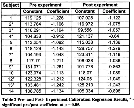
1 119.125 -1.226 107.028 -1.122 2* 113.784 -1.166 116.972 -1.075 3* 116.291 -1.164 99.556 -1.057 4* 104.838 -0.912 121.137 -0.64 5 113.254 -1.082 115.038 -1.136 6 118.129 -1.143 128.757 -1.279 7* 104.193 -1.048 123.311 -1.116 8 117.17 -1.211 106.038 -1.036 9* 131.071 -1.261 101.778 -0.863 10 123.074 -1.113 118.07 -1.089 12* 122.328 -1.212 124.05 -1.049 13* 133.481 -1.242 125.219 -1.243 14 108.785 -1.134 105.034 -0.898

Table 2 Pre- and Post- Experiment Calibration Regression Results, *=

significant pre/post coefficient at p = 0.05.

Seven of thirteen subjects had a significant pre/post coefficient according to a two-tailed t-test (Table 2). The distribution of t-values for the pre/post coefficient was shown in the

following graph (Figure 6). Notice that Subject 4's t-value was an outlier and suggested that the errors in the joystick calibration procedure were large. Since the t-values did not

appear to be biased (either positively or negatively) but to be randomly distributed, an alternative test compared the slopes of the pre- and post-experiment regressions

separately from the intercepts. A significant difference in the slopes might suggest that the subject's sensitivity to joystick deflection changed during the experiment or that a skewed error existed in the data. This would have precipitated the rejection of that subject's magnitude data as unreliable. A significant shift in the intercept would have affected all ratios equally and masked any failures of the basic hypothesis. As shown in Table 3, none of the t-test values for the slopes and intercepts were significant at the 5%

level for a two-tailed test. For each individual, the pre- and post-experiment data points were pooled to calculate a single regression line. With this linear equation, all raw joystick deflections were converted to a percentage scale for each subject's perceived

10 8 6 4 2 0 -2 -4

T-value for Pre/Post Coefficient of Calibration Curve Multiple Regression - --- --- --- -- --- 4 --- - --- --- --- --- --- --- --- --- ---0 2 4 6 8 Subject 10 12

Figure 6- T-test Values for Pre/Post Regression Variable

Slope Intercept

Subject t-test value p-value2 _{t-test value p-value}

1 0.760 0.293 -1.572 0.180 2 0.942 0.260 0.578 0.333 3 0.607 0.326 -1.662 0.172 4 2.391 0.126 2.436 0.124 5 -0.245 0.424 0.134 0.458 6 -1.035 0.245 1.375 0.200 7 -0.437 0.369 2.077 0.143 8 1.662 0.172 -1.765 0.164 9 3.194 0.097 -4.128 0.076 10 0.134 0.458 -0.474 0.359 12 1.062 0.240 0.191 0.440 13 -0.009 0.497 -1.238 0.216 14 0.995 0.251 -0.270 0.416

Table 3-Regression Parameter t-Test Values

2 For a two-tailed t-test, t>to

025 for a result to be significant at the 5% _level

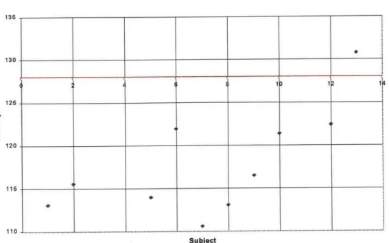
Intercept for Individual Calibration Curves

21 1D.

. ... .. ... ... .. ... ... I .. ...-...-- . -.. -

-Su bject

Figure 7-Individual Calibration Curves, Intercept Values- The ideal calibration curve has an intercept equal to 128.

Slope of Individual Calibration Curves

... ... ... . ... . ... -. . -. - .

-1>D 121

Su bject

Figure 8- Individual Calibration Curves- Slope Values calibration curve equals -1.28

The slope of the ideal 136 130 126 U 120 116 110 -1 -1.06 -1.1 -1.16 -1.2 -1.26 -1.3

were plotted in Figure 7 and Figure 8 respectively. In general, individual calibration curves underestimated the percentage joystick deflection compared to the ideal calibration curve.

Profiles

The magnitude of self-motion was plotted with time for each trial (Figure 9). Typically, after a latency period, the magnitude of self-motion increased at a constant rate and then maintained a constant level near the peak magnitude for the rest of the trial. An

occasional dropout occurred but the perceived speed of self-motion did not necessarily decline to zero. Some subjects seemed to overshoot their indication of the magnitude of self-motion and reduce the joystick deflection to a lower level. Alternatively, vection diminished after a few seconds to a stable plateau. This decay occurred more frequently at higher scene speeds. All profiles may be reviewed in Appendix E- Vection Magnitude Profiles. The subject's certainty of their motion may have influenced the slope of

perceived speed increase more than the scene velocity. The first two trials of each block were examined to determine if the subject complied with the instructions to consider the maximum self-motion on the first trial to equate 50% of the joystick scale.3 _{The profiles} indicated that many subjects underestimated their speed of self-motion when viewing the modulus. Consequently, comparing the perceived speed of self-motion between subjects was uncertain; however the analysis of within subject changes in magnitude due to scene or posture is still possible by comparing the ratios of perceived speeds for different subjects.

3 The first two trials were examined because some subjects did not attain vection on the

first trial. In these cases, the second repetition of the middle speed was designated the modulus.

Subject 1

Upright Bbck 1 Uprighl Bbek 2

100 100 g 080 Bo 60 40- * 40 .20 20 0 2 4 6 5 10 0 2 4 6 8 10 Time (s) ime (6)

Supine Bbak 1 Supine 1bak 2

100 100 60 0 40 40 'I I 20.0 2 X. 0' . o 2 4 a a 10 0 2 4 6 5 10 Time (s) lime (.) FimtTrial eecondTrial ----

-Figure 9- Typical Magnitude Profiles for the first two trials at speed 3 for each experimental block. (Recall that speed 3 was designated the modulus and the subject was instructed to deflect the joystick 50% to indicate the maximum magnitude of that trial).

Subject Variability

The number of trials during which an individual experienced vection varied with scene speed and from subject to subject (Figure 10). The development of vection was less robust at the lower speeds. In particular, Subject 3 experienced vection infrequently at all

speeds. Furthermore, during post-experiment interview, the subject described her vection as very weak and only occurring at the end of the trial. Often, she did not have enough time to indicate the magnitude of vection. This study was concerned with the

effects for subjects experiencing vection and thus it seemed reasonable to explore the results with this subject excluded.

Percent of Trials Achieving Vection per Speed

100% V 90% - -80% --70% ---0 Speed 1 0.4 m/s aSpeed 2, 0.6 mIs 50% - Speed 3, 0.8 m/s jSpeed 4. 1.1 m/s 40% *Speed S 1.6 rn/s

Figur 10 Prcen of Tials chieingdVctio

O- 40%-30% 20%-10% % -- 1 2 3 4 5 6 7 8 9 10 12 13 14 Subject

Figure 10- Percent of Trials Achieving Vection

Each vection measure was analyzed with repeated measures statistics. This analysis did not permit missing values in the data set. Therefore, empty cells due to trials with no vection were replaced by the average value of the measure for that particular subject, block, and speed. In total, 14.7% of the cells were empty. In theory, injecting average values into empty cells would reduce the degrees of freedom in the statistical analysis. This loss of degrees was not compensated for in the analysis. The substitution should not have greatly affected the results since the number of degrees of freedom was large.

Furthermore, many of the calculations were redone with Subject 3 omitted and the percentage of empty cells in the data set was reduced. Although the variability in the data was artificially reduced, so were the likely effects of speed and posture and therefore the results would be erring on the conservative side of the hypothesis. It was possible that vection would have occurred in some of the missing trials had the trial continued beyond the 10 second trial length. Consequently, the substitution for missing data M

reduced the mean values of the measures of subjects with a substantial number of missed trials. The substitution also distorted adaptation trends linked to repetition of the

stimulus.

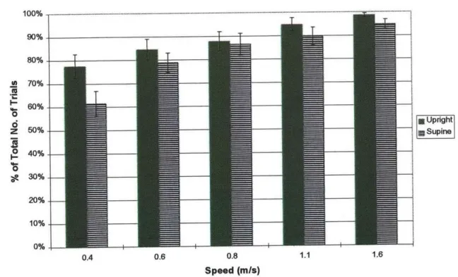
Posture also influenced the average number of trials achieving vection. Subjects

experienced vection at all speeds more frequently when upright (Figure 11). The overall difference between upright and supine posture was significant ( F(l,12) = 5.225,

p= 0.041). The greatest difference occurred at the lowest speed. No significant

difference between blocks was observed (F(1,12)= 0.898, p=0.3 6 2).

No. of Trials with Vection as a Function of Posture

4') 'U I-6e~ 0 z 0 I- I.-0 100%. 90%. 80%- 70%-60%. 50%. 40%. 30%. 20%-10%. Upriht 0% 4-0.4 0.6 0.8 Speed (m/s) 1.1 1.6

Figure 11- Number of Trials with Vection as a Function of Posture

T - T :- I

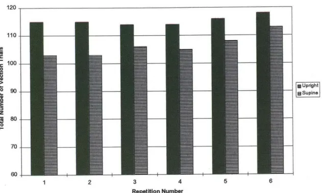
No of trials vs Repetition Number 120- 110-.2 ₁₀₀ -> 0 Upriht 90 E z ~80-70 1 2 3 4 5 6 Repetition Number

Figure 12- Number of Vection Trials as a Function of Presentation Order

For each vection measure, the data set was structured as a three factor repeated measures analysis across Repetition (4 levels), Posture and Block (4 levels), and Speed (5 levels). Each subject observed 6 repetitions of each stimulus level but Systat allowed a maximum of 99 data points per case for a repeated measures analysis. The last four repetitions were chosen because fewer trials, and therefore, fewer degrees of freedom were missing from that data subset (Figure 12). Finally, for each measure, the means of the first four repetitions and that of the last four repetitions were plotted to ensure that the choice of

data sets did not influence the results (Appendix D- Early and Late Repetitions

Compared) The General Linear Model method (Systat V. 7) was used to model the mean latencies of the repeated measures.

Latency

Latencies (Figure 13 and Figure 14) decreased with speed (F(4, 44 )= 13.654; p = 0.0). The subject means were slightly positively skewed but their distribution was close to

normal. Individually, nine of thirteen subjects showed an inversely proportional trend between latency and speed. Posture exerted a significant influence on latency

(F(1, 1l)= 5.609, p = 0.037). The difference between postures diminished at the higher

speeds (Figure 15). The order of presentation of postures did not produce a significant effect on the results (F(1,11)=0.594, p=0.457). (Note that the subject means were coarsely distributed about the mean for each speed).

Average Vection Latency- Upright Posture

10 -U U, 6 -J 9 8 7 6 6 3 2 1 0.4 0.6 0.8 1.2 1.4 1.6 Speed (m/s)

Figure 13-Latencies vs. Speed, Upright Posture4

4_{Unless specified, all error bars indicate the standard error of the mean.}

0 U S

-F-

Average Vection Latency - Supine Posture 10 9 8 0.6 0.8 1.2 1.4 Speed (mis)

Figure 15- Mean Latencies Upright and Supine Compared

a

S

-3

0.4 0.6 0.8 1 1.2 1.4 1.6

Speed (m/s)

Figure 14-Latencies vs. Speed, Supine Condition

Average Vection Latency -Upright and Supine Compared

(Subject 3 Omitted) 6 -----...-...-... -... -...-- -...-...-... S 6 5 4 0 A S U C * Subject Means .- Speed Mean .Upright -... Supln 1.6 6 4 3.5 -3 0.4 --- --- --- --- -- --- --- -- ---- ~---. --- --- -.. ---. --- - -..- -- -- -- ---- - ----- --- -- -- - --- --- - --- - - - --- - --- -. 6 4.6

-Maximum Magnitude

As shown in Figure 16 and Figure 17, the variance of the magnitude values increased with scene speed in violation of one of the underlying assumptions of ANOVA. The values were transformed by a power relationship in order to stabilize the variance with scene speed (Figure 18 and Figure 19). All peak magnitude values were raised to the power of 0.325. Then, the transformed magnitude data set was analyzed by repeated measures statistics to uncover any significant posture or speed effects. The overall and

subjects means for the peak magnitudes were displayed in logarithmic plots for each posture separately (Figure 20 and Figure 21). These two plots confirmed the skewness of

the range of subjects means and the dependence of the variance on scene speed. For both postures, the maximum magnitude (Figure 22) increased with speed (F(4,44) = 50.584,

p = 0.0). Neither order of presentation (F(1,11) = 0.343, p = 0.570) nor posture

150 100 MAXMAG 50 01L 0.0

Figure 16- Box Plot of Maximum Magnitude Distribution vs. Speed, Supine Posture

' The length of each box indicates the range within which the central 50% of the values

fall. The mean is represented by the line partitioning the box. The hinges mark the limits of the first and third quantiles. The asterisks denote outliers.

* * 0.5 1.0 SPEED 1.5 2.0 I I

150 100 I MAXMAG 50 0 0. 0 0.5 1.0 SPEED

Figure 17- Box Plot of Maximum Magnitude Distribution vs. Posture Speed, Upright 5 4 3 RANSMAG 2 1 0I 0. 0 0.5 1.0 SPEED

Figure 18- Box Plot of Transformed Maximum Magnitude Distribution vs. Speed, Upright Posture - --*** 1.5 2.0 S-1.5 2.0 w M- M.

TRANSMAG 5 4 3 2

1

Figure 19-Box plot of Maximum Transformed Magnitude Distribution v. Speed-Supine Posture

Subject Means for Maximum Magnitude Upright Posture

Subject mean +I---+ Uprdght Mean

Speed(ns)

Figure 20-Maximum Magnitude vs. Speed, Upright Posture

IT I. I

10

10*

10

Subject Means for Maximum Magnitude Supine Posture

Subjectr

Supine Nmean ean- ,

10 Speed(rris)

Figure 21- Maximum Magnitude vs. Speed, Supine Posture

Means of Transformed Maximum Magnitude- Postures Compared . -..._-.. --- - - -- --- - - - -- _ _ _. --- - - - -0.6 0.8 1 1.2 1.4 - Upright ...Supine 1.6 Speed (m/s)

Figure 22-Maximum Magnitude, Supine and Upright Compared

10? 10 d) C~1 10: 3.5 3 to 2 .5 E E E 0.5 0 0.4

Area Under the Curve

Area increased with the scene speed (F(4,44) = 47.206, p = 0.0). This result was

expected since maximum magnitude also increased with speed, and latency decreased. Figure 23 indicated that area was slightly greater upright than the supine; however, this difference was not statistically significant (F(1, 11) = 1.890, p = 0.197). The order of presentation did not influence the results (F(1, 11) =0.004, p = 0.954).

Mean Area, Upright and Supine Postures Compared

'U S 4 300 250 200 IS0 100 60 0 0.4 0.8 0.8 1.2 1.4 ~Urightiio~ Supne I. Speed (m/s)

Figure 23- Mean Area, Upright and Supine Postures Compared Rise Time

The rise time was defined as the time from the onset of vection to 90% of the peak vection magnitude. The order of presentation showed no significant main effect

(F(1,l1)= 0.159, p= 0.698). Speed had a significant effect (F(4, 44)= 5.492, p= 0.003).

The difference in rise time between the lowest and the highest speed in the upright

...... ..-- - ~ ... - ... ... -- --... .... -- --- . --.~ ~ ..-.... ..- -

Rise Time Means- Upright and Supine Postures

0.8 1.2

1.-.

Speed (m/s)

Figure 24- Mean Rise Time, Upright and Supine Postures Compared

posture is approximately 1.0 s while for supine the increase is about 0.7 s. Upright mean rise times are longer than for the supine posture (F(1,11) = 4.969, p = 0.048).

Rise Slope

The slope increased with speed (F(4,44) = 16.587, p = 0.0) with indications of a plateau at higher speeds (Figure 25). Neither posture (F(1,12) = 0.037, p = 0.850) nor order of presentation (F(l, 11) = 0.341, p = 0.571) were statistically significant factors. Similar

to the maximum magnitude results, the slope values were transformed by raising the values to the power of 0.1 in order to stabilize the variance with scene speed.

3 2.5 2 r 1.6 0. L0 0.5 0 0.4 0.6 .-...

W-