Publisher’s version / Version de l'éditeur:
Vous avez des questions? Nous pouvons vous aider. Pour communiquer directement avec un auteur, consultez la première page de la revue dans laquelle son article a été publié afin de trouver ses coordonnées. Si vous n’arrivez pas à les repérer, communiquez avec nous à [email protected]. Questions? Contact the NRC Publications Archive team at
[email protected]. If you wish to email the authors directly, please see the first page of the publication for their contact information.
https://publications-cnrc.canada.ca/fra/droits
L’accès à ce site Web et l’utilisation de son contenu sont assujettis aux conditions présentées dans le site LISEZ CES CONDITIONS ATTENTIVEMENT AVANT D’UTILISER CE SITE WEB.
Human Language Technology Conference: North American Chapter of the
Association for Computational Linguistics Annual Meeting (HLT/NAACL 2006)
[Proceedings], 2006
READ THESE TERMS AND CONDITIONS CAREFULLY BEFORE USING THIS WEBSITE.
https://nrc-publications.canada.ca/eng/copyright
NRC Publications Archive Record / Notice des Archives des publications du CNRC :
https://nrc-publications.canada.ca/eng/view/object/?id=d91d8d1e-2ad7-4710-9e57-1b902811e2a1 https://publications-cnrc.canada.ca/fra/voir/objet/?id=d91d8d1e-2ad7-4710-9e57-1b902811e2a1
NRC Publications Archive
Archives des publications du CNRC
This publication could be one of several versions: author’s original, accepted manuscript or the publisher’s version. / La version de cette publication peut être l’une des suivantes : la version prépublication de l’auteur, la version acceptée du manuscrit ou la version de l’éditeur.
Access and use of this website and the material on it are subject to the Terms and Conditions set forth at
Segment Choice Models: Feature-Rich Models for Global Distortion in
Statistical Machine Translation
Kuhn, Roland; Yuen, D.; Simard, Michel; Paul, P.; Foster, George; Joanis,
Eric; Johnson, John Howard
National Research Council Canada Institute for Information Technology Conseil national de recherches Canada Institut de technologie de l'information
Segment Choice Models : Feature-Rich
Models for Global Distortion in Statistical
Machine Translation *
Kuhn, R., Yuen, D., Simard, M., Paul, P., Foster, G., Joanis,
E., and Johnson, H.
June 2006
* published at the Human Language Technology Conference - North American Chapter of the Association for Computational Linguistics Annual Meeting (HLT/NAACL 2006). New York City, New York, USA. June 5, 2006. pp 25-32. NRC 48752.
Copyright 2006 by
National Research Council of Canada
Permission is granted to quote short excerpts and to reproduce figures and tables from this report, provided that the source of such material is fully acknowledged.
Segment Choice Models: Feature-Rich Models for Global
Distortion in Statistical Machine Translation
Roland Kuhn, Denis Yuen, Michel Simard, Patrick Paul,
George Foster, Eric Joanis, and Howard Johnson
Institute for Information Technology, National Research Council of Canada Gatineau, Québec, CANADA
Email: {Roland.Kuhn, Michel.Simard, Patrick.Paul, George.Foster, Eric.Joanis, Howard.Johnson}@cnrc-nrc.gc.ca; Denis Yuen: [email protected]
Abstract
This paper presents a new approach to distortion (phrase reordering) in phrase-based machine translation (MT). Distor-tion is modeled as a sequence of choices during translation. The approach yields trainable, probabilistic distortion models that are global: they assign a probability to each possible phrase reordering. These “segment choice” models (SCMs) can be trained on “segment-aligned” sentence pairs; they can be applied during decoding or rescoring. The approach yields a metric called “distortion perplexity” (“disperp”) for comparing SCMs offline on test data, analogous to perplexity for language models. A decision-tree-based SCM is tested on Chinese-to-English translation, and outperforms a baseline distortion penalty approach at the 99% confidence level.
1
Introduction: Defining SCMs
The work presented here was done in the context of phrase-based MT (Koehn et al., 2003; Och and Ney, 2004). Distortion in phrase-based MT occurs when the order of phrases in the source-language sentence changes during translation, so the order of corresponding phrases in the target-language trans-lation is different. Some MT systems allow
arbi-trary reordering of phrases, but impose a distortion penalty proportional to the difference between the new and the original phrase order (Koehn, 2004). Some interesting recent research focuses on reor-dering within a narrow window of phrases (Kumar and Byrne, 2005; Tillmann and Zhang, 2005; Till-mann, 2004). The (TillTill-mann, 2004) paper intro-duced lexical features for distortion modeling. A recent paper (Collins et al., 2005) shows that major gains can be obtained by constructing a parse tree for the source sentence and then applying hand-crafted reordering rules to rewrite the source in target-language-like word order prior to MT.
Our model assumes that the source sentence is completely segmented prior to distortion. This simplifying assumption requires generation of hy-potheses about the segmentation of the complete source sentence during decoding. The model also assumes that each translation hypothesis grows in a predetermined order. E.g., Koehn’s decoder (Koehn 2004) builds each new hypothesis by add-ing phrases to it left-to-right (order is deterministic for the target hypothesis). Our model doesn’t re-quire this order of operation – it would support right-to-left or inwards-outwards hypothesis con-struction – but it does require a predictable order.
One can keep track of how segments in the source sentence have been rearranged during de-coding for a given hypothesis, using what we call a “distorted source-language hypothesis” (DSH). A similar concept appears in (Collins et al., 2005) (this paper’s preoccupations strongly resemble
ours, though our method is completely different: we don’t parse the source, and use only automati-cally generated rules). Figure 1 shows an example of a DSH for German-to-English translation (case information is removed). Here, German “ich habe das buch gelesen .” is translated into English “i have read the book .” The DSH shows the distor-tion of the German segments into an English-like word order that occurred during translation (we tend to use the word “segment” rather than the more linguistically-charged “phrase”).
Figure 1. Example of German-to-English DSH From the DSH, one can reconstruct the series of segment choices. In Figure 1 - given a left-to-right decoder - “[ich]” was chosen from five candidates to be the leftmost segment in the DSH. Next, “[habe]” was chosen from four remaining candi-dates, “[gelesen]” from three candicandi-dates, and “[das buch]” from two candidates. Finally, the decoder was forced to choose “[.]”.
Segment Choice Models (SCMs) assign probabilities to segment choices made as the DSH is constructed. The available choices at a given time are called the “Remaining Segments” (RS). Consider a valid (though stupid) SCM that assigns equal probabilities to all segments in the RS. This uniform SCM assigns a probability of 1/5! to the
DSH in Figure 1: the probability of choosing “[ich]” from among 5 RS was 1
/5, then the
probability of “[habe]” among 4 RS was 1/4 , etc.
The uniform SCM would be of little use to an MT system. In the next two sections we describe some more informative SCMs, define the “distortion perplexity” (“disperp”) metric for comparing SCMs offline on a test corpus, and show how to construct this corpus.
2
Disperp and Distortion Corpora
2.1 Defining Disperp
The ultimate reason for choosing one SCM over another will be the performance of an MT system containing it, as measured by a metric like BLEU (Papineni et al., 2002). However, training and
testing a large-scale MT system for each new SCM would be costly. Also, the distortion component’s effect on the total score is muffled by other components (e.g., the phrase translation and target language models). Can we devise a quick standalone metric for comparing SCMs?
There is an offline metric for statistical language models: perplexity (Jelinek, 1990). By analogy, the higher the overall probability a given SCM assigns to a test corpus of representative distorted sentence hypotheses (DSHs), the better the quality of the SCM. To define distortion perplexity (“disperp”), let PrM(dk) = the probability an SCM M assigns to
a DSH for sentence k, dk. If T is a test corpus
comprising numerous DSHs, the probability of the corpus according to M is PrM(T) = k PrM(dk).
Let S(T) = total number of segments in T. Then
disperp(M,T) = PrM(T) -1/S(T)
. This gives the mean number of choices model M allows; the lower the disperp for corpus T, the better M is as a model for T (a model X that predicts segment choice in T perfectly would have disperp(X,T) = 1.0).
2.2 Some Simple A Priori SCMs
The uniform SCM assigns to the DSH dk that has
S(dk) segments the probability 1/[S(dk)!] . We call
this Model A. Let’s define some other illustrative SCMs. Fig. 2 shows a sentence that has 7 segments with 10 words (numbered 0-9 by original order). Three segments in the source have been used; the decoder has a choice of four RS. Which of the RS has the highest probability of being chosen? Per-haps [2 3], because it is the leftmost RS: the “left-most” predictor. Or, the last phrase in the DSH will be followed by the phrase that originally followed it, [8 9]: the “following” predictor. Or, perhaps positions in the source and target should be close, so since the next DSH position to be filled is 4, phrase [4] should be favoured: the “parallel” pre-dictor.
Figure 2. Segment choice prediction example Model B will be based on the “leftmost” predic-tor, giving the leftmost segment in the RS twice the probability of the other segments, and giving the
Original German: [ich] [habe] [das buch] [gelesen] [.] DSH for German: [ich] [habe] [gelesen] [das buch] [.]
(English: [i] [have] [read] [the book] [.])
original: [0 1] [2 3] [4] [5] [6] [7] [8 9] DSH: [0 1] [5] [7], RS: [2 3], [4], [6], [8 9]
others uniform probabilities. Model C will be based on the “following” predictor, doubling the probability for the segment in the RS whose first word was the closest to the last word in the DSH, and otherwise assigning uniform probabilities. Fi-nally, Model D combines “leftmost” and “follow-ing”: where the leftmost and following segments are different, both are assigned double the uniform probability; if they are the same segment, that segment has four times the uniform probability. Of course, the factor of 2.0 in these models is arbi-trary. For Figure 2, probabilities would be:
• Model A: PrA([2 3])= PrA([4])= PrA([6])= PrA([8 9]) = 1/4; • Model B: PrB ([2 3])= 2/5, PrB([4])= PrB([6])= PrB([8 9]) = 1/5; • Model C: PrC ([2 3])= PrC ([4])= PrC([6]) = 1/5, PrC([8 9]) = 2/5; • Model D: PrD ([2 3]) = PrD([8 9]) = 1/3, PrD([4])= PrD([6]) = 1/6.
Finally, let’s define an SCM derived from the distortion penalty used by systems based on the “following” predictor, as in (Koehn, 2004). Let ai =
start position of source phrase translated into ith target phrase, bi -1= end position of source phrase
that’s translated into (i-1)th target phrase. Then distortion penalty d(ai, bi-1) = ¦ai– bi-1 -1¦; the total
distortion is the product of the phrase distortion penalties. This penalty is applied as a kind of non-normalized probability in the decoder. The value of
for given (source, target) languages is optimized on development data.
To turn this penalty into an SCM, penalties are normalized into probabilities, at each decoding stage; we call the result Model P (for “penalty”). Model P with = 1.0 is the same as uniform Model A. In disperp experiments, Model P with optimized on held-out data performs better than Models A-D (see Figure 5), suggesting that dis-perp is a realistic measure.
Models A-D are models whose parameters were all defined a priori; Model P has one trainable pa-rameter, ✁ . Next, let’s explore distortion models with several trainable parameters.
2.3 Constructing a Distortion Corpus
To compare SCMs using disperp and to train complex SCMs, we need a corpus of representative examples of DSHs. There are several ways of ob-taining such a corpus. For the experiments de-scribed here, the MT system was first trained on a bilingual sentence-aligned corpus. Then, the sys-tem was run in a second pass over its own training corpus, using its phrase table with the standard dis-tortion penalty to obtain a best-fit phrase alignment between each (source, target) sentence pair. Each such alignment yields a DSH whose segments are aligned with their original positions in the source; we call such a source-DSH alignment a “segment alignment”. We now use a leave-one-out procedure to ensure that information derived from a given sentence pair is not used to segment-align that sen-tence pair. In our initial experiments we didn’t do this, with the result that the segment-aligned cor-pus underrepresented the case where words or N-grams not in the phrase table are seen in the source sentence during decoding.
3
A Trainable Decision Tree SCM
Almost any machine learning technique could be used to create a trainable SCM. We implemented one based on decision trees (DTs), not because DTs necessarily yield the best results but for soft-ware engineering reasons: DTs are a quick way to explore a variety of features, and are easily inter-preted when grown (so that examining them can suggest further features). We grew N DTs, each defined by the number of choices available at a given moment. The highest-numbered DT has a “+” to show it handles N+1 or more choices. E.g., if we set N=4, we grow a “2-choice”, a “3-choice”, a “4-choice”, and a “5+-choice tree”. The 2-choice tree handles cases where there are 2 segments in the RS, assigning a probability to each; the 3-choice tree handles cases where there are 3 seg-ments in the RS, etc. The 5+-choice tree is differ-ent from the others: it handles cases where there are 5 segments in the RS to choose from, and cases where there are more than 5. The value of N is arbitrary; e.g., for N=8, the trees go from “2-choice” up to “9+-“2-choice”.
Suppose a left-to-right decoder with an N=4 SCM is translating a sentence with seven phrases. Initially, when the DSH is empty, the 5+-choice tree assigns probabilities to each of these seven. It
will use the 5+-choice tree twice more, to assign probabilities to six RS, then to five. To extend the hypothesis, it will then use the 4-choice tree, the 3-choice tree, and finally the 2-3-choice tree. Disperps for this SCM are calculated on test corpus DSHs in the same left-to-right way, using the tree for the number of choices in the RS to find the probability of each segment choice.
Segments need labels, so the N-choice DT can assign probabilities to the N segments in the RS. We currently use a “following” labeling scheme. Let X be the original source position of the last word put into the DSH, plus 1. In Figure 2, this was word 7, so X=8. In our scheme, the RS seg-ment whose first word is closest to X is labeled “A”; the second-closest segment is labeled “B”,
etc. Thus, segments are labeled in order of the (Koehn, 2004) penalty; the “A” segment gets the lowest penalty. Ties between segments on the right and the left of X are broken by first labeling the right segment. In Figure 2, the labels for the RS are “A” = [8 9], “B” = [6], “C” = [4], “D” = [2 3].
Figure 3. Some question types for choice DTs Figure 3 shows the main types of questions used for tree-growing, comprising position questions and word-based questions. Position questions pertain to location, length, and ordering of seg-ments. Some position questions ask about the dis-tance between the first word of a segment and the “following” position X: e.g., if the answer to “pos(A)-pos(X)=0?” is yes, then segment A comes immediately after the last DSH segment in the source, and is thus highly likely to be chosen. There are also questions relating to the “leftmost” and “parallel” predictors (above, sec. 2.2). The fseg() and bseg() functions count segments in the
RS from left to right and right to left respectively, allowing, e.g., the question whether a given seg-ment is the second last segseg-ment in the RS. The only word-based questions currently implemented ask whether a given word is contained in a given segment (or anywhere in the DSH, or anywhere in the RS). This type could be made richer by allow-ing questions about the position of a given word in a given segment, questions about syntax, etc.
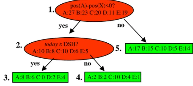
Figure 4 shows an example of a 5+-choice DT. The “+” in its name indicates that it will handle cases where there are 5 or more segments in the RS. The counts stored in the leaves of this DT rep-resent the number of training data items that ended up there; the counts are used to estimate probabili-ties. Some smoothing will be done to avoid zero probabilities, e.g., for class C in node 3.
Figure 4. Example of a 5+-choice tree
For “+” DTs, the label closest to the end of the alphabet (“E” in Figure 4) stands for a class that can include more than one segment. E.g., if this 5+-choice DT is used to estimate probabilities for a 7-segment RS, the segment closest to X is labeled “A”, the second closest “B”, the third closest “C”, and the fourth closest “D”. That leaves 3 segments, all labeled “E”. The DT shown yields probability Pr(E) that one of these three will be chosen. Cur-rently, we apply a uniform distribution within this “furthest from X” class, so the probability of any one of the three “E” segments is estimated as Pr(E)/3.
To train the DTs, we generate data items from the second-pass DSH corpus. Each DSH generates several data items. E.g., moving across a seven-segment DSH from left to right, there is an exam-ple of the seven-choice case, then one of the six-choice case, etc. Thus, this DSH provides three items for training the 5+-choice DT and one item
pos(A)-pos(X)<0? A:27 B:23 C:20 D:11 E:19
today DSH?
A:10 B:8 C:10 D:6 E:5
A:8 B:6 C:0 D:2 E:4 A:2 B:2 C:10 D:4 E:1
A:17 B:15 C:10 D:5 E:14 yes no yes no 1. 3. 2. 5. 4. 1. Position Questions Segment Length Questions
E.g., “lgth(DSH)<5?”, “lgth(B)=2?”, “lgth(RS)<6?”, etc.
Questions about Original Position
Let pos(seg) = index of seg’s first word in source sentence
E.g., “pos(A)=9?”, “pos(C) <17?”, etc.
Questions With X (“following” word position)
E.g., “pos(X)=9?”, “pos(C) – pos(X) <0?”, etc.
Segment Order Questions
Let fseg = segment # (forward), bseg = segment # (back-ward)
E.g., “fseg(D) = 1?”, “bseg(A) <5?”, etc. 2. Word-Based Questions
E.g., “and ✁
DSH?”, “November ✁
each for training the 4-choice, 3-choice, and 2-choice DTs. The DT training method was based on Gelfand-Ravishankar-Delp expansion-pruning (Gelfand et al., 1991), for DTs whose nodes con-tain probability distributions (Lazaridès et al., 1996).
4
Disperp Experiments
We carried out SCM disperp experiments for the English-Chinese task, in both directions. That is, we trained and tested models both for the distortion of English into Chinese-like phrase order, and the distortion of Chinese into English-like phrase or-der. For reasons of space, details about the “dis-torted English” experiments won’t be given here. Training and development data for the distorted Chinese experiments were taken from the NIST 2005 release of the FBIS corpus of Xinhua news stories. The training corpus comprised 62,000 FBIS segment alignments, and the development “dev” corpus comprised a disjoint set of 2,306 segment alignments from the same FBIS corpus. All disperp results are obtained by testing on “dev” corpus.
Distorted Chinese: Models A-D, P, & a four-DT Model 1 2 3 4 5 6 7 8 500 1000 2000 4000 8000 1600 0 3200 0 6200 0
# training alignments (log scale)
D is p e rp o n " d e v " Model A Model B Model C Model D Model P (alpha = 0.77) Four DTs: pos + 100-wd qns
Figure 5. Several SCMs for distorted Chinese Figure 5 shows disperp results for the models described earlier. The y axis begins at 1.0 (mini-mum value of disperp). The x axis shows number of alignments (DSHs) used to train DTs, on a log scale. Models A-D are fixed in advance; Model P’s single parameter was optimized once on the en-tire training set of 62K FBIS alignments (to 0.77) rather than separately for each amount of training
data. Model P, the normalized version of Koehn’s distortion penalty, is superior to Models A-D, and the DT-based SCM is superior to Model P.
The Figure 5 DT-based SCM had four trees (2-choice, 3-(2-choice, 4-(2-choice, and 5+-choice) with position-based and word-based questions. The word-based questions involved only the 100 most frequent Chinese words in the training corpus. The system’s disperp drops from 3.1 to 2.8 as the num-ber of alignments goes from 500 to 62K.
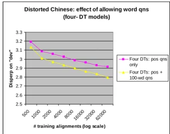
Figure 6 examines the effect of allowing word-based questions. These questions provide a signifi-cant disperp improvement, which grows with the amount of training data.
Distorted Chinese: effect of allowing word qns (four- DT models) 2.5 2.6 2.7 2.8 2.9 3 3.1 3.2 3.3 500 1000 2000 4000 8000 1600 0 3200 0 6200 0
# training alignments (log scale)
D is p e rp o n " d e v " Four DTs: pos qns only Four DTs: pos + 100-wd qns
Figure 6. Do word-based questions help? In the “four-DT” results above, examples with five or more segments are handled by the same “5+-choice” tree. Increasing the number of trees allows finer modeling of multi-segment cases while spreading the training data more thinly. Thus, the optimal number of trees depends on the amount of training data. Fixing this amount to 32K alignments, we varied the number of trees. Figure 7 shows that this parameter has a significant im-pact on disperp, and that questions based on the most frequent 100 Chinese words help perform-ance for any number of trees.
Distorted Chinese: Disperp vs. # of trees (all trees grown on 32K alignments)
2.3 2.4 2.5 2.6 2.7 2.8 2.9 3 3.1 3.2 3 4 5 6 7 8 9 10 11 12 13 14 # of trees D is p e rp o n " d e v " pos qns only pos + 100-wd qns
Figure 7. Varying the number of DTs
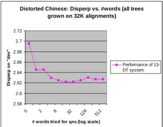
In Figure 8 the number of the most frequent Chinese words for questions is varied (for a 13-DT system trained on 32K alignments). Most of the improvement came from the 8 most frequent words, especially from the most frequent, the comma “,”. This behaviour seems to be specific to Chinese. In our “distorted English” experiments, questions about the 8 most frequent words also gave a significant improvement, but each of the 8 words had a fairly equal share in the improvement.
Distorted Chinese: Disperp vs. #words (all trees grown on 32K alignments) 2.58 2.6 2.62 2.64 2.66 2.68 2.7 2.72 0 2 8 32 128 512
# words tried for qns (log scale)
D is p e rp o n " d e v " Performance of 13-DT system
Figure 8. Varying #words (13-DT system) Finally, we grew the DT system used for the MT experiments: one with 13 trees and questions about the 25 most frequent Chinese words, grown on 88K alignments. Its disperp on the “dev” used for the MT experiments (a different “dev” from the one above – see Sec. 5.2) was 2.42 vs. 3.48 for the baseline Model P system: a 30% drop.
5
Machine Translation Experiments
5.1
SCMs for Decoding
SCMs assume that the source sentence is fully segmented throughout decoding. Thus, the system must guess the segmentation for the unconsumed part of the source (“remaining source”: RS). For the results below, we used a simple heuristic: RS is broken into one-word segments. In future, we will apply a more realistic segmentation model to RS (or modify DT training to reflect accurately RS treatment during decoding).
5.2
Chinese-to-English MT Experiments
The training corpus for the MT system’s phrase tables consists of all parallel text available for the NIST MT05 Chinese-English evaluation, except the Xinhua corpora and part 3 of LDC's “Multiple-Translation Chinese Corpus” (MTCCp3). The Eng-lish language model was trained on the same cor-pora, plus 250M words from Gigaword. The DT-based SCM was trained and tuned on a subset of this same training corpus (above). The dev corpus for optimizing component weights is MTCCp3. The experimental results below were obtained by testing on the evaluation set for MTeval NIST04.
Phrase tables were learned from the training cor-pus using the “diag-and” method (Koehn et al., 2003), and using IBM model 2 to produce initial word alignments (these authors found this worked as well as IBM4). Phrase probabilities were based on unsmoothed relative frequencies. The model used by the decoder was a log-linear combination of a phrase translation model (only in the P(source|target) direction), trigram language model, word penalty (lexical weighting), an op-tional segmentation model (in the form of a phrase penalty) and distortion model. Weights on the components were assigned using the (Och, 2003) method for max-BLEU training on the develop-ment set. The decoder uses a dynamic-programming beam-search, like the one in (Koehn, 2004). Future-cost estimates for all distortion mod-els are assigned using the baseline penalty model. 5.3
Decoding Results
29,40 29,60 29,80 30,00 30,20 30,40 30,60 30,80 31,00 31,20 no PP PP no PP PP DP DT B L E U s c o re 1x beam 4x beam
Figure 9. BLEU on NIST04 (95% conf. = ±0.7) Figure 9 shows experimental results. The “DP” systems use the distortion penalty in (Koehn, 2004) with optimized on “dev”, while “DT” systems use the DT-based SCM. “1x” is the default beam width, while “4x” is a wider beam (our notation reflects decoding time, so “4x” takes four times as long as “1x”). “PP” denotes presence of the phrase penalty component. The advantage of DTs as measured by difference between the score of the best DT system and the best DP system is 0.75 BLEU at 1x and 0.5 BLEU at 4x. With a 95% bootstrap confidence interval of ±0.7 BLEU (based on 1000-fold resampling), the resolution of these results is too coarse to draw firm conclusions.
Thus, we carried out another 1000-fold bootstrap resampling test on NIST04, this time for pairwise system comparison. Table 1 shows results for BLEU comparisons between the systems with the default (1x) beam. The entries show how often the A system (columns) had a better score than the B system (rows), in 1000 observations.
A vs. B ✁ DP, no PP DP, PP DT, no PP DT, PP DP, no PP x 2.95% 99.45% 99.55% DP, PP 97.05% x 99.95% 99.95% DT, no PP 0.55% 0.05% x 65.68% DT, PP 0.45% 0.05% 34.32% x
Table 1. Pairwise comparison for 1x systems
The table shows that both DT-based 1x systems performed better than either of the DP systems more than 99% of the time (underlined results). Though not shown in the table, the same was true with 4x beam search. The DT 1x system with a phrase penalty had a higher score than the DT 1x system without one about 66% of the time.
6
Summary and Discussion
In this paper, we presented a new class of probabil-istic model for distortion, based on the choices made during translation. Unlike some recent dis-tortion models (Kumar and Byrne, 2005; Tillmann and Zhang, 2005; Tillmann, 2004) these Segment
Choice Models (SCMs) allow phrases to be moved globally, between any positions in the sentence. They also lend themselves to quick offline com-parison by means of a new metric called disperp. We developed a decision-tree (DT) based SCM whose parameters were optimized on a “dev” cor-pus via disperp. Two variants of the DT system were experimentally compared with two systems with a distortion penalty on a Chinese-to-English task. In pairwise bootstrap comparisons, the sys-tems with DT-based distortion outperformed the penalty-based systems more than 99% of the time.
The computational cost of training the DTs on large quantities of data is comparable to that of training phrase tables on the same data - large but manageable – and increases linearly with the amount of training data. However, currently there is a major problem with DT training: the low pro-portion of Chinese-English sentence pairs that can be fully segment-aligned and thus be used for DT training (about 27%). This may result in selection bias that impairs performance. We plan to imple-ment an alignimple-ment algorithm with smoothed phrase tables (Johnson et al. 2006) to achieve segment alignment on 100% of the training data.
Decoding time with the DT-based distortion model is roughly proportional to the square of the number of tokens in the source sentence. Thus, long sentences pose a challenge, particularly dur-ing the weight optimization step. In experiments on other language pairs reported elsewhere (Johnson
et al. 2006), we applied a heuristic: DT training and decoding involved source sentences with 60 or fewer tokens, while longer sentences were handled with the distortion penalty. A more principled
ap-proach would be to divide long source sentences into chunks not exceeding 60 or so tokens, within each of which reordering is allowed, but which cannot themselves be reordered.
The experiments above used a segmentation model that was a count of the number of source segments (sometimes called “phrase penalty”), but we are currently exploring more sophisticated models. Once we have found the best segmentation model, we will improve the system’s current naïve single-word segmentation of the remaining source sentence during decoding, and construct a more accurate future cost function for beam search. An-other obvious system improvement would be to incorporate more advanced word-based features in the DTs, such as questions about word classes (Tillmann and Zhang 2005, Tillmann 2004).
We also plan to apply SCMs to rescoring N-best lists from the decoder. For rescoring, one could apply several SCMs, some with assumptions dif-fering from those of the decoder. E.g., one could apply right-to-left SCMs, or “distorted target” SCMs which assume a target hypothesis generated the source sentence, instead of vice versa.
Finally, we are contemplating an entirely differ-ent approach to DT-based SCMs for decoding. In this approach, only one DT would be used, with only two output classes that could be called “C” and “N”. The input to such a tree would be a par-ticular segment in the remaining source sentence, with contextual information (e.g., the sequence of segments already chosen). The DT would estimate the probability Pr(C) that the specified segment is “chosen” and the probability Pr(N) that it is “not chosen”. This would eliminate the need to guess the segmentation of the remaining source sentence.
References
P. Brown, S. Della Pietra, V. Della Pietra, and R. Mer-cer. 1993. “The Mathematics of Statistical Machine Translation: Parameter Estimation”. Computational
Linguistics, 19(2), pp. 263-311.
M. Collins, P. Koehn, and I. Ku erová. 2005. “Clause Restructuring for Statistical Machine Translation”.
Proc. ACL, Ann Arbor, USA, pp. 531-540.
S. Gelfand, C. Ravishankar, and E. Delp. 1991. “An Iterative Growing and Pruning Algorithm for Clas-sification Tree Design”. IEEE Trans. Patt. Analy.
Mach. Int. (IEEE PAMI), V. 13, no. 2, pp. 163-174. F. Jelinek. 1990. “Self-Organized Language Modeling
for Speech Recognition” in Readings in Speech
Recognition (ed. A. Waibel and K. Lee, publ. Mor-gan Kaufmann), pp. 450-506.
H. Johnson, F. Sadat, G. Foster, R. Kuhn, M. Simard, E. Joanis, and S. Larkin. 2006. “PORTAGE: with Smoothed Phrase Tables and Segment Choice Mod-els”. Submitted to NAACL 2006 Workshop on
Statis-tical Machine Translation, New York City.
P. Koehn. 2004. “Pharaoh: a Beam Search Decoder for Phrase-Based Statistical Machine Translation Mod-els”. Assoc. Machine Trans. Americas (AMTA04). P. Koehn, F.-J. Och and D. Marcu. 2003. “Statistical
Phrase-Based Translation”. Proc. Human Lang.
Tech. Conf. N. Am. Chapt. Assoc. Comp. Ling. (NAACL03), pp. 127-133.
S. Kumar and W. Byrne. 2005. “Local Phrase Reorder-ing Models for Statistical Machine Translation”.
HLT/EMNLP, pp. 161-168, Vancouver, Canada. A. Lazaridès, Y. Normandin, and R. Kuhn. 1996.
“Im-proving Decision Trees for Acoustic Modeling”.
Int. Conf. Spoken Lang. Proc. (ICSLP96), V. 2, pp. 1053-1056, Philadelphia, Pennsylvania, USA. F. Och and H. Ney. 2004. “The Alignment Template
Approach to Statistical Machine Translation”.
Comp. Linguistics, V. 30, Issue 4, pp. 417-449. Franz Josef Och. 2003. “Minimum Error Rate Training
for Statistical Machine Translation”. Proc. ACL, Sapporo, Japan.
K. Papineni, S. Roukos, T. Ward, and W.-J. Zhu. 2002. “BLEU: A method for automatic evaluation of ma-chine translation”. Proc. ACL, pp. 311-318. C. Tillmann and T. Zhang. 2005. “A Localized
Predic-tion Model for Statistical Machine TranslaPredic-tion”.
Proc. ACL.
C. Tillmann. 2004. “A Block Orientation Model for Statistical Machine Translation”. HLT/NAACL. S. Vogel, H. Ney, and C. Tillmann. 1996. “HMM-Based
Word Alignment in Statistical Translation”.