Adaptive control of hypersonic vehicles

Adaptive Control of Hypersonic Vehicles

by

Travis Eli Gibson

Submitted to the Department of Mechanical Engineering

in partial fulfillment of the requirements for the degree of

Master of Science

at the MAK U 0 ZUU

MASSACHUSETTS INSTITUTE OF TECHNOLOJY

Yk U

ARIES

September 2008

@ Massachusetts Institute of Technology 2008. All rights reserved.

Author ...

Department of Mechanical Engineering

August 15, 2008

Certified by ...

Anuradha M. Annaswamy

Senior Research Scientist

Thesis Supervisor

<1

A ccepted by ...

Lallit Anand

Chairman, Department Committee on Graduate Students

ARCHIVES

i

MA (AiH IUSETTS INSTITUTE

Adaptive Control of Hypersonic Vehicles

by

Travis Eli Gibson

Submitted to the Department of Mechanical Engineering on August 15, 2008, in partial fulfillment of the

requirements for the degree of Master of Science

Abstract

The guidance, navigation and control of hypersonic vehicles are highly challenging tasks due to the fact that the dynamics of the airframe, propulsion system and struc-ture are integrated and highly interactive. Such a coupling makes it difficult to model various components with a requisite degree of accuracy. This in turn makes var-ious control tasks including altitude and velocity command tracking in the cruise phase of the flight extremely difficult. This work proposes an adaptive controller for a hypersonic cruise vehicle subject to: aerodynamic uncertainties, center-of-gravity movements, actuator saturation, failures, and time-delays. The adaptive control ar-chitecture is based on a linearized model of the underlying rigid body dynamics and explicitly accommodates for all uncertainties. Within the control structure is a base-line Proportional Integral Filter commonly used in optimal control designs. The control design is validated using a highfidelity HSV model that incorporates various effects including coupling between structural modes and aerodynamics, and thrust pitch coupling. Analysis of the Adaptive Robust Controller for Hypersonic Vehicles (ARCH) is carried out using a control verification methodology. This methodology illustrates the resilience of the controller to the uncertainties mentioned above for a set of closed-loop requirements that prevent excessive structural loading, poor track-ing performance, and engine stalls. This analysis enables the quantification of the improvements that result from using and adaptive controller for a typical maneuver in the V-h space under cruise conditions.

Thesis Supervisor: Anuradha M. Annaswamy Title: Senior Research Scientist

Acknowledgments

I would like to thank Dr. Anuradha Annaswamy for her continued support in my research endeavors. I believe we will continue to generate great work together. Thank you as well to Dr. Luis Crespo of the NIA for his research support. His work has helped to illustrate the benefits of my research. I would also like to thank Dr. Sean Kenny at NASA Langley for his direction during my summer work. I would like to thank my lab mates: Yildiray Yildiz, Dr. Jinho Jang, Zac Dydek, Megumi Matsutani and Manohar Srikanth. And of course my mom dad and brother for relaxing times back in Florida. Finally I would like to thank God for helping me through my long nights in lab, and these intense semesters at MIT.

Contents

1 Introduction

1.1 History of X-Planes . . ...

1.2 Modelling of Hypersonic Vehicles . ... 1.3 Control Design . .... ... 1.4 Overview ... ... ...

2 Vehicle Modelling

2.1 Oblique Shock and Expansion Wave Theory . . . . 2.2 Rigid Body Forces and Moments . . . ...

2.3 Elastic Forces and Moments . ...

2.3.1 Natural Modes of Vibration for a Fixed-Free 2.3.2 Forced Modal Response . ...

2.4 Equations of Motion . ... 2.4.1 Evaluation Model . ... 2.4.2 Design Model . .... 2.4.3 Actuator Dynamics ... 3 Controller Design 3.1 Linear Model ... 3.2 Baseline Controller . ...

3.3 Uncertainties and Actuator Saturation

3.4 Adaptive Controller . . . .... 15 16 18 20 . . . . . .. . 21 Beam 23 24 26 32 33 36 37 38 .. . . . 41 . . . . . . 42 43 .. . . . 43 .. . . . 45 . . . . . . . . . 47 .. . . . 49

4 Simulation Studies

5 Control Verification, A different Approach 63

5.1 Mathematical Framework . . . ... ... .... 63

5.2 Hypersonic Vehicle Uncertainty ... . . . 65

5.3 Baseline Controller Analysis ... .... 67

5.4 Adaptive Controller Analysis ... .... 67

5.5 Comparative Analysis ... ... .. 68 6 Conclusions 71 A Tables 73 B Figures 77 B.1 Simulation Study-N1 ... ... 78 B.2 Simulation Study-Al ... ... 81 B.3 Simulation Study-N2 ... ... . 84 B.4 Simulation Study-A2 ... ... . 87 B.5 Simulation Study-N3 ... ... . 90 B.6 Simulation Study-A3 ... ... . 93 B.7 Simulation Study-N4 ... ... . 96 B.8 Simulation Study-A4 ... ... . 99

List of Figures

HSV side view with control inputs[7]... HSV side view with dimenion labels[7]... Visual aids for oblique shock and Prandtl-Meyer Mach Number Location Subscript Indexing .

Scramjet Model[7] . ...

Elastic HSV beam model with coordinates. . Forward and aft mode shape . ... Axes of the HSV ...

expansion.

PIF control structure . ... Nominal control structure ... Uncertainty modelling ...

Nominal with adaptive augmentation and uncertainty Error Modelling . ...

Pole Zero Map for 5 Se to V -y...

Pole Zero Map zoom in at the origin ... Reference command in h-V space. ...

Command following errors for N1 and Al simulation studies. Control input for N1 and Al simulation studies . . . . .

Command following errors for N2 and A2 simulation studies. Control input for N2 and A2 simulation studies ...

Command following errors for N3 and A3 simulation studies. Control input for N3 and A3 simulation studies . . . . .

Command following errors for N4 and A4 simulation studies. 4-11 Control input for N4 and A4 simulation studies . . . . 5-1 Failure and non-failure domains for the adaptive controller.

N1 Control inputs . . . . . .

N1 Command following error. N1 Rigid states . . . . ...

N1 Loading Factor . . . . N1 Adaptive parameters. . . . Al Control inputs . . . . . .

Al Command following error. Al Rigid states . . . .... Al Loading Factor . . . . . .

Al Adaptive parameters. . . . N2 Control inputs . . . . . .

N2 Command following error. N2 Rigid states . . . ... N2 Loading Factor . . . . . .

N2 Adaptive parameters. . . . A2 Control inputs . . . . . .

A2 Command following error. A2 Rigid states . . . ... A2 Loading Factor . . . . . . A2 Adaptive parameters. . . . 4-4 4-5 4-6 4-7 4-8 4-9 4-10 57 57 58 58 59 60 60 61 B-i B-2 B-3 B-4 B-5 B-6 B-7 B-8 B-9 B-10 B-11 B-12 B-13 B-14 B-15 B-16 B-17 B-18 B-19 B-20 .. . . . . 78 .. . . . . . . . . . 78 .. . . . . 79 .. . . . 80 .. . . . . . . . 80 .. . . . . 81 ._{. . . . . . . .} . 8 1 .. . . . . 82 .................. . . . . 8 3 .. . . . . . . . 83 ............... . . . . . 8 4 .. . . . . . . . . . 84 ............... . . . . . 8 5 .. . . . 86 .. . . . . . . 86 ............... . . . . . 8 7 ._{. . . . .} . . . . 8 7 .................. . . . . 8 8 .. . . . . . 89 . . . . 8 9

. . . . . . . . . . . . . 9 0

B-22 N3 Command following error ... 90

B-23 N3 Rigid states. ... . ... .. 91

B-24 N3 Loading Factor. ... ... ... 92

B-25 N3 Adaptive parameters. . ... ... 92

B-26 A3 Control inputs. ... . ... .. 93

B-27 A3 Command following error. ... ... 93

B-28 A3 Rigid states. ... ... 94

B-29 A3 Loading Factor. ... ... ... 95

B-30 A3 Adaptive parameters. ... ... 95

B-31 N4 Control inputs. ... . ... .. 96

B-32 N4 Command following error. ... ... 96

B-33 N4 Rigid states. ... ... . . 97

B-34 N4 Loading Factor. ... ... 98

B-35 N4 Adaptive parameters. ... ... 98

B-36 A4 Control inputs. ... . ... .. 99

B-37 A4 Command following error. . ... ... 99

B-38 A4 Rigid states. . ... ... 100

B-39 A4 Loading Factor . ... ... . 101

B-40 A4 Adaptive parameters. ... ... 101

List of Tables

4.1 Trim values for two input HSV model. . ... . . 53

4.2 Simulation Study Uncertainty Selection. . ... . . 56

5.1 1-dimensional CPVs for dbase . . . . . . . . . . . 67

5.2 1-dimensional CPVs for dadaptive . ... ... . 68

5.3 Relative PSM improvement. . ... .... 68

A.1 Geometry of Aircraft. ... . . ... 73

A.2 Physical Constants and Aerodynamic Coefficients. [40, 20] ... 74

A.3 Trim values for two input HSV model. ... ... 75

A.4 Eigenvalues and Modes of HSV. . ... .. 75

Chapter 1

Introduction

"Not since the Right Brothers solved the basic problems of sustained, controlled flight has there been such an assault upon our atmosphere as during the first years of the space age. Man extended and speeded up his travels within the vast ocean of air surrounding the Earth until he achieved flight outside its confines. This remarkable accomplishment was the culmination of a long history of effort to harness the force of that air so that he could explore the three-dimensional ocean of atmosphere in which he lives. That history had shown him that before he could ex-plore his ethereal ocean, he must first exex-plore the more restrictive world of aerodynamic forces." [46]

Wendell H. Stillwell

In attempts to slice through the air at higher and higher speeds, ever more elegant and abstract aircraft designs have been conjured by NASA engineers and scientist. The X-43 is one such aircraft, Figure 1-3. This aircraft is a flying butter knife. One can imagine controlling it is not an easy task. Rear control surfaces, strong engine-airframe coupling and flexibility effects each compound the control problem, and the problem is exacerbated at hypersonic speeds. In this work an adaptive control algorithm is presented that has superior performance and robustness characteristics

when compared to a nominal classic controller.

1.1

History of X-Planes

The National Advisory Committee for Aeronautics (NACA) started the United States X-Plane Program in 1945 with the XS-1, later designated X-1, Figure 1-1. A contract was given to Bell Aircraft Inc., and oversight on the program was managed by the United States Air Force. The goal of the project was to break the sound barrier with a manned aircraft. On October 14th 1947 that was accomplished. [48, 37] Projects like this have continued ever since. Out of the X-Plane program the first aircrafts to fly at altitudes exceeding 100,000, 200,000 and 300,000 ft, along with the first aircrafts to fly at Mach 3, 4, 5, and 6 have been built and tested.1

Figure 1-1: Bell X-1

One of the most notable projects to come out of the program is the X-15 aircraft, Figure 1-2. The program began in 1954 and 199 test flights were performed. The X-15 was designed with several research goals in mind. The major goal was to understand the effects of high speed atmosphere reentry. In the process the X-15 broke altitude and speed records with flights higher than 300,000 ft and at speeds in

excess of Mach 6.[30] The results of this project directly impacted the short 7 years before Alan Shepard was the first American in space.

Figure 1-2: X-15

Two important characteristics of the X-15 program were the exploration of the hypersonic regime and the implementation of an adaptive algorithm in aircraft stabi-lization. "The Hypersonic Envelope, starts at a Mach number like 5 and extends to a Mach number or velocity as high as the imagination and technology will allow." [38] This quote by Richard Neumann illustrates the somewhat vague nature of the term "hypersonic". The hypersonic flight regime is particulary important for the X-43 as that is the defining characteristic that allows for the efficient combustion of the scramjet engine. This will be discussed in more detail in a subsequent section.

The adaptive control algorithm implemented in the X-15 project was designed by Minneapolis Honeywell Corp. It was referred to as a "Self-Adaptive" control system. The Self-Adaptive control system had a variable feedback gain on euler rates in order to maintain attitude stability in flight. The variable feedback gains were adjusted so as to minimize the error between the actual attitude of the aircraft and some ideal reference attitude. The adaptive controller decreased the tuning time necessary to gain schedule a classic controller over the entire flight envelope.[46, 18]

The adaptive algorithm from Honeywell was truly ahead of its time in implemen-tation. However, it lacked the mathematical tools necessary to prove stability in a rigorous manner and relied on "rule of thumb" ideologies instead. This ended in tragedy however. On November 15, 1967 test flight 191 of 199 crashed above Delamar

Dry Lake.[30] Unbeknownst to the pilot there was an electrical malfunction and the aircraft began to deviate from the desired trajectory and a gross side-slip angle was building. Once off by 150 _{the pilot corrected for the mistake, then the aircraft drifted}

again, after several seconds of pilot corrections the aircraft interred a Mach 5 spin at an altitude of 230,000 ft.[30, 47] As the aircraft fell into more dense air it broke apart killing the pilot, Mike Adams. This crash put a holt on all adaptive control implementation for several decades, and not until recently has the idea been revisited. Now with more rigorous stability proofs.

In an attempt to pave the way for reusable and more affordable vehicles the X-43 program was initiated in order to conduct experiments in hypersonic vehicle system identification and inflight scramjet combustion. The first flight was in 2001, Figure 1-3.[36, 51] Airbreathing hypersonic engines are being considered because of the reduced weight of such systems when compared to rocket powered hypersonic vehicles. Rockets require that the oxidizer along with the fuel be carried up with the aircraft. Where as in a scramjet engine, the oxidizer is not needed. This can potentially increase the payload capabilities of scramjet powered vehicles.

Figure 1-3: X-43 artistic rendering

1.2

_{Modelling of Hypersonic Vehicles}

The X-43 could not launch from the ground and the scramjet engine was not operable unless at hypersonic speeds. The typical mission profile would be as follows. The

X-43 begins attached to the end of a Pegasus Rocket and both structures together would be carried under the wing of a B-52B, see Figure 1-4. The B-52B would carry the Pegasus booster system up to an altitude of 40,000 ft where the Pegasus booster would be dropped. The booster would then propel the X-43 to an altitude of 95,000 ft at some hypersonic speed where the X-43 would then be pushed off the end of the Pegasus Rocket. Then, depending on the mission objectives, the X-43 would carry out various tasks. This mission profile is illustrated in Figure 1-5. The dynamics of the X-43 after the Pegasus push-off are what this work pertains to. This flight condition will be referred to as the cruise condition for the X-43.

Figure 1-4: X-43 on Pegasus under B-52B [6]

Several attempts have been made to characterize the longitudinal dynamics of a hypersonic vehicle. One notable comprehensive analytical aeropropilsive-aeroelastic

Hypersonic Vehicle (HSV) model is that proposed by Chavez and Schmidt in [10].

In that work a 2-D vehicle geometry was assumed; and with Newtonian theory, a

1-D isentropic scramjet model, and a lumped mass elastic model the HSV dynamics

were formulated. Newtonian theory, however, is better suited for blunt bodies and becomes less accurate for slender bodies. Noting this fact, Bolender and Doman

X-43A Mission Pr

Figure 1-5: X-43 flight envelope [5]

in [7] propose an HSV model that builds upon the work by Chavez. Instead of Newtonian Impact theory, Oblique Shock theory is proposed for the compression of high speed air. Bolender and Doman's work incorporates the elastic effects with a double cantilever beem model, and the rigid-elastic dynamics are then obtained through a Lagrangian formulation. Doman and Bolender have recently built upon their work in [7] and included unsteady, thermal, and viscous effects as well as an updated elastic model. [9]. CFD-based characterizations have also been proposed such as that in [11].

1.3

Control Design

The Guidance, Navigation and Control of hypersonic vehicles are highly challenging tasks due to the fact that the dynamics of the airframe, propulsion and structure are highly integrated and highly interactive. Such a coupling makes it very difficult to model various components with a requisite degree of accuracy. This in turn makes

various control tasks including altitude and velocity command tracking in the cruise phase of the flight extremely difficult.

Notable works in the area of HSV control design are discussed here in. In [33], an adaptive linear-quadratic controller is deployed in the presence of structural modes and actuator dynamics, and is shown to track altitude and velocity commands in the presence of aerodynamic changes and actuator changes. The authors of [52] designed an adaptive sliding mode controller that tracks step commands in height and velocity while requiring limited state information. In [19] the authors employed both robust and adaptive techniques on a sequential loop closing methodology. The work in [31] focuses on elastic mode suppression through an adaptive notch filter technique. References [35], [49] and [50] not only focus on control design but also on robustness characteristics of the controller. Similar studies are carried out in this thesis in Chapter 5. Other notable works in the area of control of Hypersonic vehicles are References [34, 1, 26, 13, 12, 24, 41, 39, 23, 40, 42] and [32].

Uncertainty characterization is also important when determining the relative ro-bustness characteristics of any given controller. Aircraft geometry and mass property uncertainties have been studied in [39]. Aerodynamics coefficient uncertainties were used in [40] and [33] to test the control algorithm; and inertial-elastic uncertainties were studied in [42] and [28].

1.4

Overview

In this work, a baseline controller is first developed that has Proportional, Integral and Filter components, commonly called a PIF controller. [44] An adaptive controller then augments to the baseline controller. It accommodates for aerodynamic uncer-tainties, center-of-gravity movements, actuator saturation and failures and is robust with respect to time-delays and elastic effects. The nonlinear rigid HSV model in

[40] is used for control design and the nonlinear aeroelastic HSV model in [7] is used for controller evaluation. Time simulations are presented to illustrate the benefits of the adaptive algorithm. Analysis is also performed in order to study the resilience

of the controller to the uncertainties mentioned above for a set of closed-loop re-quirements that prevent excessive structural loading, poor tracking performance and engine stalls.[21, 22]

Chapter

Vehicle Modelling

The Hypersonic Vehicle, HSV, geometry used in this study is shown in Figure 2-1. This geometry is representative of the NASA X-43 aircraft. There are three control inputs for this vehicle, the elevator deflection S,, the canard deflection 6, and the equivalence ratio for the fuel in the scramjet ¢. The canard was added in recent studies in order to increase the available bandwidth for the controller. [8, 40] It should be noted however that this control surface may not be physically realizable given the harsh environment in the forward of the aircraft. For that reason the HSV model is constructed so that the canard effects can easily be removed, so as to have a two input system. In order to obtain the physics based model proposed in this work the pressure

Elevator

B o s o k. S c r a m j e t : f ( )

Reflected shock % Shear Layer Cowl Door - --- SLayer

Figure 2-1: HSV side view with control inputs[7]

distribution around the aircraft must be defined. Then, the rigid(elastic) forces are obtained by integration of the pressure distribution over the surface(mode shapes)

i Id Sla

Forward Under-side Aft

Figure 2-2: HSV side view with dimenion labels[7]

of the HSV. Given the simple geometry of the aircraft, a majority of the pressure distribution can be obtained by implementing Prandtl-Meyer expansion and oblique shock theory.

2.1

Oblique Shock and Expansion Wave Theory

Oblique shock theory is applicable when supersonic flow is turned over a concave surface, see Figure 2-3 for physical intuition. Given a prescribed turn angle 6t the shock angle 0~ can be calculated with the following expression,

sin6 0, + bsin4 _{80, + csin}2 _{O~ + d = 0, (2.1)}

where M= - sin2 6t 2M2 +1 ( + 1)2 - ] c = M4 + + sin2 t (2.2) Cos2 6t d=. _M4

In the previous expression M1 denotes the mach number of the fluid before reaching

the shock wave and y represents the ratio of specific heats (-y = C,/C,). The shock angle is then determined by solving for the second root of Equation (2.1) with respect to sin2 0s. The pressure p, temperature T, and Mach number M, can then be obtained

using the relations,

P2 7M, sin2 08 -1 Pi 6 T2 (7M? sin2 0 - 1) (M sin2 s + 5) T, 36 M sin 0,

S(0

,

M

sin2

82

+

5

-where subscripts 1 and 2 denote pre and post shock values.[3]

(2.3) (2.4) (2.5) Shock Line :, I 8 c

MI

Oblique Shock Theory

Constant Entropy Expansion Fan

I j S< M2 T1> T2

0

0

Figure 2-3: Visual aids for oblique shock and Prandtl-Meyer expansion.[2] When the opposite scenario occurs and flow is turned over a convex corner, the flow expands. The properties of the gas are then characterized by Prandtl-Meyer expansion, 6t = v(M 2) - v(M) (2.6) where (2.7) y+1 +1 v(M)= arctan (M 2 _{-_ 1) arctan M}2 _{- 1.}

7-1

V -i

calculated as, 3]

P2 _ 1 + [(y - 1)/2]M / ) (2.8)

Pi 1+ [(y - 1)/2]M22

T2 1 + [(y - 1)/2]M2 (2.9)

T, 1 + [(- - 1)/2] M22

These theories can then be applied across the front, top and bottom of the aircraft in order to obtain the pressure distribution for the upper-surface, forward, underside, and inlet to the scramjet as well as the air properties around the canard and elevator.

2.2

Rigid Body Forces and Moments

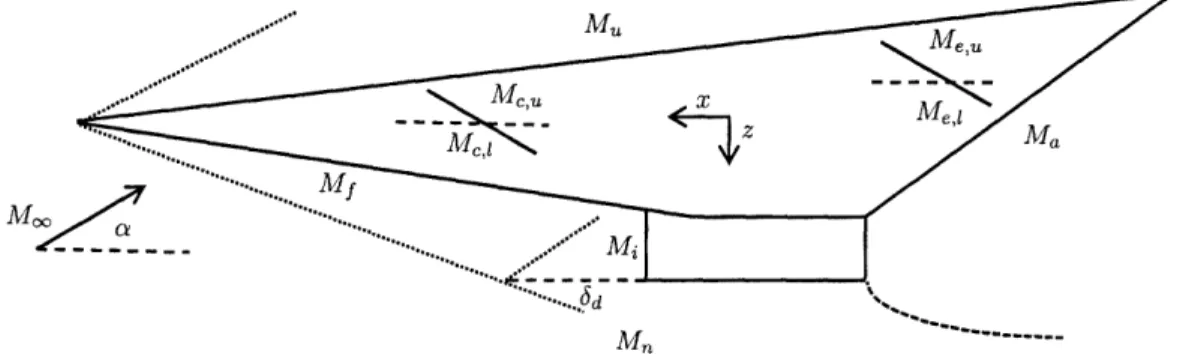
Given the free stream Mach Number Mo, temperature T,,, and and air pressure poo, the location of the bow shock can be determined along with the upper body properties on the top of the air frame and the forward lower body properties, as shown in Figure 2-4. Note that the following subscript notation (.), and (.)f will be used to denote upper-body properties and forward under-body properties respectively.

Once the pressures are determined as described above, the forces and moments on the upper-side of the HSV are found as,

Fx,, = -pulu tan 1r,_u (2.10)

Fz,u = PUIU (2.11)

My,U = ZfF x,, - cJf F,u, (2.12)

where iu and i are the differences between the geometric center of the upper panel

moments on the forward under-side are then found using the following expressions,

Fx,f = -pfll tan T11 , (2.13)

Fz,f = -Pf ll (2.14)

My,, = fFx,f - I7;Fy,f, (2.15)

with 2f and Xf having the same interpretation as above. The pressure is constant on the surface of the HSV behind the bow shock and it is for that reason that the forces are simply calculated using a single value for the pressure across the entire surface.

MMM

Figure 2-4: Mach Number Location Subscript Indexing

The air after passing through the bow shock on the under-side of the HSV will impinge on the cowl door, which protrudes in front of the scramjet engine. The cowl door is assumed to be adjustable and in this work it is assumed that the cowl door can be adjusted perfectly so as to maintain an on lip condition with the bow shock wave. Given this scenario, there will be a force exerted on the aircraft as the post bow shock air is turned parallel to the entrance of the scramjet,

Fx,inlet Mpf(1 f= - cos(T1,z + ac))hi (2.16) Fz,inlet = yM2pf sin(TI, + a)hi (2.17)

Iy,inlet = inletFx,inlet - i inletFz,inlet. (2.18)

expression,

ld = If - (If tan 71,1 + hi) cot(6d - a), (2.19)

where 6d is the relative angle between the bow shock and the cowl door, and a is the angle of attack of the aircraft.

The nacelle is the cowl door and the underside of the scramjet together, and properties of the aircraft under the nacelle are denoted as (-),. The nacelle length is given as,

In = ls + ld.

The total force and moment imparted on the nacelle of the aircraft is determined by the following relations,

Fz,n = -pnl (2.20)

MY,n = -Fz,n,;n, (2.21)

where i~ is distance between the center of the nacelle and the center of gravity of the aircraft, and p, is calculated using either oblique shock theory or expansion theory depending on the angle of attack. Note that given the shock on lip condition, the properties for the nacelle are simply determined from the free stream air. If the shock on lip condition is not satisfied, the above relations do not hold.

Continuing to follow the path of the air, after passing through the bow shock and then the second shock from the reflection on the cowl door, the air will enter the scramjet engine. The scramjet is modelled as 1-D, and isentropic flow is assumed. The expressions necessary to incorporate the propulsion system were first introduced by Chavez and Schmidt. [10] The model for the scramjet is shown in Figure 2-5. After the free stream air impinges on the cowl it is turned upward parallel to the entrance of the scramjet. Oblique Shock theory can be used in order to determine the Mach Number at the Inlet from the Mach Number under the fore-body of the HSV.

Reflecting Shock Wayve .

/. Diffuser Combustor Nozzle

M hi hi hce he Mf ./

_M

Figure 2-5: Scramjet Model[7]

as,

1 + [(-1)/2]M2 ]( _+)/(-)

1M2ci

= 1 + [( - 1)/2]M] )/

d

M2?

where (.)i denotes the inlet to the scramjet, (.),i denotes the combustor inlet, and Ad is the diffuser area ratio as shown in Figure 2-5. The air properties at the combustor inlet are calculated using Equations (2.8) and (2.9).

The combustor is modelled as a constant area duct with heat addition. This leads to the expression,

M [1 + [(y - 1)/2]Mce]

(7M2e + 1)2

M,1 + [(7 - 1)/2]M,] M2 2 Tt

(yM

M + 1)2

_{M + 1)2}

_Tc,

where the Mach number at the combustor exit Me is a function of the total tem-perature change across the combustor ATt. The temtem-perature and pressure at the combustor exit are then defined as

Pce = Pci 1

+ 7~c M

(2.24)

(2.25)

An analytical expression relating the total temperature change across the com-(2.22)

bustor to the equivalence ratio q follows,

T c 1 +i Hfrcf.stO/(cpTtc

_{= .}

_(2.26)

Ttei 1 + fsTO5

ATtc = Ttce - T (2.27)

where r; is the efficiency of the scramjet (0.9), fst is the stoichiometric air-fuel ratio (0.0291), H, is the heat of combustion for the fuel (LH2 at 51,500 BTU/lbm) and cp is the specific heat of the fuel at constant pressure (0.24 BTU/(lbm°R).[25, 27, 4, 7]

It is important to note that temperatures with subscript t are the total temperatures and all other temperatures referred to in this work are the static temperatures. The ratio of total temperature to static temperature can be obtained using the following,

Tt y- 1

= 1 + M2. (2.28)

T 2

The procedure for obtaining the Mach number for the air at the exit of the scramjet is similar to that of Equation (2.22),

[1 -+ [( - 1)/2]M2 (1)/1y-1) 1 + [( - 1)/2]M2e( y1)/(-)

= A2 (2.29)

Using a control volume around the scramjet and applying the law of conservation of momentum, the total thrust from the scramjet can be obtained

T = riTa(V - V.) + (Pe - p.)he - (pi - p.)hi. (2.30) The air upon leaving the scramjet will then expand along the aft of the aircraft and interact with the free stream air coming from the underside of the HSV. An analytical expression for the pressure on the aft of the scramjet as a function of the free stream air pressure was found by Chavez and Schmidt and is displayed below,

pa = _{1 + Sa/la(Pe/Poo} Pe _{- 1)} (2.31)

where la is the length of the aft of the aircraft in the x-body direction and sa is the length coordinate in the x-body direction. Integration of the aft body pressure along the back side of the aircraft results into the following expressions for the aft-body forces and moments,

Pe log(pe/poo)

Fx,a = Poola Pe og( tan(T2 + 71,u) (2.32)

Fz,a = -oola og(p/p) (2.33)

Poo (Pe/Poo) - 1

My,a - aFx,a - aFz,a (2.34)

where the pitching moment is calculated from the point of average pressure on the aft

body panel. The point of average pressure can be calculated as 1a = fa Pa(sa)dsa/la

The center of pressure coordinates are then found by solving for Xa in the following expression Pa(Xa) = pa. Then the relative position of the center of pressure to the center of gravity of the HSV is trivial.

Two components of the total force acting on the HSV that have not been ad-dressed yet are the forces from the canard and elevator. Depending on the angle of attack of the HSV and the relative positions of the canard and elevator the pressure surrounding the control surfaces can be determined from oblique shock or Prandtl-Meyer expansion. Once the pressures surrounding the canard are determined, the forces acting upon it are calculated as follows,

Fx,c = - (Pc,l - Pc,u) sin S6CS (2.35)

Fz,c = - (Pc,, - Pc,u) cos 6cSc (2.36)

MY,C = cFx,c - ;cFz,c. (2.37)

below for completeness,

Fx,e = - (Pe,i - Pe,u) sin 6eSe (2.38) Fz,e = - (Pe,i - Pe,u) cos 6eSe (2.39)

My,e =Fx,e - -ez,e. (2.40)

For the coordinates of the canard and elevator refer to Appendix A. 1.

Thus far all of the forces and moments acting on the hypersonic vehicle that control the rigid-body dynamics have been expressed and therefore the total x-body force, z-body force and y-body moment are calculated as follows,

Fx = Fx,u + F,f + Fx,iniet + Fx,a + Fx,e + F,c (2.41) Fz = F,u + F,f + Fz,iniet + z,n Fz,a + Fz,e + Fz,c (2.42)

My = M,, + M,,f + My,iniet + M,, + My,a + My,e + My,, + z T. (2.43)

As previously mentioned, this work also includes the elastic effects an the HSV dy-namics. These effects are outlined in the following section.

2.3

Elastic Forces and Moments

The elastic effects are obtained by modelling the HSV as two fixed free beams. One beam free at the forward of the HSV and fixed at the center of gravity, and a second beam fixed at the center of gravity and free toward the aft. A visual representation of the above beam model is shown in Figure 2-6. It is important to note that the

coordinate system for the elastic model has up as positive, where in the rigid-body model down is positive.

2.3.1

Natural Modes of Vibration for a Fixed-Free Beam

Given the above flexible beam model for the HSV, and assuming that small deflections occur so that Hooke's Law can be used, the vertical deflection y is well defined as a function of space and time. It is governed by the following partial-differential equation,

4 y(,t) 2 y(,t)

EI

814

at2

where ri is the constant mass density and EI is the constant Young's modulus area moment of inertia. For values of these parameters refer to Tables A.1 and A.2. It is assumed that the solution to (2.44) can be separated in space and time so that,

y(x, t) = (x) f (t). (2.45)

Given this, (2.44) can be separated as follows,

EIdlo4 ( ) - w2ri(x) = 0 (2.46)

dx4

df(t)

dt4 _{) + 2f(t) = 0. (2.47)}

dt4

For notational convenience the following substitution is made 34 = w2fh/EI.

Equa-tion (2.46) is now of the form,

EId4(x) 340(x) = 0. (2.48)

dx4

The solution to the ordinary-differential equation in (2.48) is referred to as the mode shape and has a solution of the following form,

The equations given thus far are for a generic free-fixed beam. The following discus-sion will pertain to the component of the elastic model forward of the HSV's center of gravity, and a later discussion will pertain to the aft section of the beam model.

The modal analysis for the forward components will be denoted with a subscript

f.

Of() = 0 (2.50)

'() = 0 (2.51) The geometric boundary conditions arise from the fact that the beam model is fixed at the center of gravity of the HSV. Also, a pair of natural boundary conditions arise at the free end of the beam,

k"(0) =0 (2.52)

"'(0)= 0. (2.53) The natural boundary conditions arise from the fact that the bending moment and shear force are both zero at the free end. Substitution of the four boundary conditions for the forward beam into the mode shape function described in (2.49), result into the following relation,

cos/3fj cosh 3fx = -1. (2.54) There are infinitely many solutions for 3f in (2.54). The infinitely many solutions

relate to the fact that a non finite number of modes determine the flexible nature of a beam. For this study only the smallest value of 3f was used and thus, only one

bending mode will be incorporated for the forward beam. Note, that the same is done for the aft beam as well. Substitution of the solution f into (2.49) results into the

following expression for the forward beam mode shape,

qf =Af [(sin Of 2 - sinh ofpt) (sin of x + sinh Pfx) + (coS f2 + cosh Pf) (cos/3_{fx + cosh f x)],}

(2.55)

where Af is a scaling factor that is chosen so as to mass normalize the mode shape and is determined by the following orthogonal solution,

J0

A similar approach was taken for the aft cantilever beam. With its unique set of four boundary conditions, the following relation results

cos(,a(1 - 2)) cosh(3a(1 - 2)) = -1,

so that the aft beam has a mode shape of the following form,

qa =Aa[(sin/3a(1 - 2) - sinh 3a(1 - 2))(sin Oa(x - 2) - sinh /3(x - 2))

+ (COS /a(l - 2) + cosh Oa(1 - 2))(cos Oa(X - 2) - cosh)a(x - 2))].

The aft beam is also mass normalized, and Aa is solved for in the following,

J a $a(X) a(x)dx = 1.

(2.57)

(2.58)

(2.59)

Using the above approach, the following values were obtained for the forward and aft beams,

Af = 0.0283 ft

Aa = -0.0256 ft

Of = 0.0341 ft-'

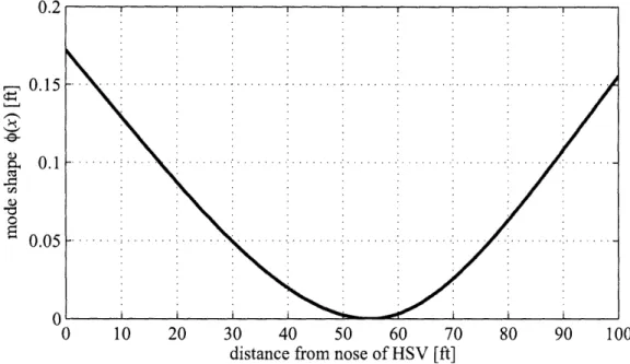
A visual representation of the combined forward and aft mode shapes as described in (2.55) and (2.58) is shown in Figure 2-7.

0.2

0.15

0.1

0.05

0 10 20 30 40 50 60 70 80 90 100

distance from nose of HSV [ft] Figure 2-7: Forward and aft mode shape.

2.3.2

Forced Modal Response

The forced response associated with (2.44) is of the form,

EI4_y(x,t)

O4 + 2y( _Ot2,t) p(x, t) + P(x, _t)6(x - _Xj),

where p denotes pressure and P is a point load. The above equation has solutions for

00

y(x, t) = Zlk( )7k (t). k=1

(2.61) where the infinite summation over k illustrates the fact that there are infinitely many modes for a fixed-free beam. Do not confuse that with the subscripts f and a. The discussion thus far has not distinguished between forward and aft, and is of a generic flavor. The r terms will later be regarded as the flexible state variables, and are

y as,

governed by the following second order equation

ilk + Wkl7k = Nk(t) (2.62)

where Nk is the modal force defined as,

1

Nk (t) = k (x)p(x, t)dx + k(j)Pj(t). (2.63)

j=1

Once again, the flexible model used in this work only pertains to the first bending modes for each beam. Application of (2.63) to the forward and aft beams results in the following force relations

Nf (t) = -

j

Na(t) = -

J

2.4

Equations of Motion

Two distinct aircraft models will be introduced in this study. One aircraft model will incorporate the flexible effects and will be used for controller evaluation, and as so will be referred to as the Evaluation Model (EM). The second model will only include the rigid-body effects and will be used for control design, and will be referred to as the Design Model (DM). The construction and implementation of these models is discussed below.

2.4.1

Evaluation Model

Using Lagrange's Equations, the equations of motion of the flexible hypersonic vehicle can be derived as follows,[7]

Fx = mU + mQW + mg sin 0 + Q(Aarla + Af7f) + 2Q(Aia + A f7f)

Fz = mW - mQU - mgcos +0 + Aaa + Af' i -2 Q2(ai7a + Af 7ff)

(I

= ( + 7+ + 7 (U + QW)(Aa7a + Af Tnf) + 2Q(7/a + '7i7f - a - Of rf

Nf = i + (W- QU)Af - Q +f +2( +wfr;f + (w2 -Q2

Na = i - (W - QU)Aa - ,)a + 2(waia + ( - Q2)qa,

(2.66)

where

Af j snfof(x)dx

Xa 7i aa(X)dX

=f X - t)qf of (x)dx

The left hand side of the equation contains the rigid and elastic forces and the pitching

moment. These forces in turn depend on the attitude of the aircraft as well as the

three control inputs. On the right hand sides of the equations are the constants, elastic coefficients and the state variables of the aircraft in the body axes. The state variables in the body axes are: pitch angle 0, pitch rate Q, body axis horizontal speed

U, and body axis vertical speed W, along with the four generalized elastic variables

r

7_7f, 7_{f, ra and la. Subscripts f and a correspond to the forward and aft of the}

aircraft respectively. The forces and moments on the left hand side are determined using rigid-body forces in (2.41)-(2.43) and the elastic force relations in (2.64) and

the following kinematic relation,

h = U sinO - W cos (2.67)

is introduced.

The implementation of Equation (2.66) is cumbersome and slow on any computer. Some of the solutions for obtaining the pressure distribution and subsequent forces on the hypersonic vehicle require solving nonlinear equations. A more implementable aircraft model is obtained through the transformation of the above system to the

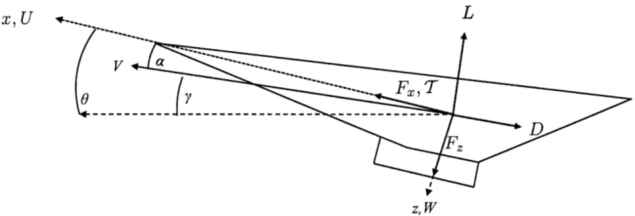
stability axis and then the subsequent curve fitting of the forces and moments to that of an algebraic relation. This increases the ease of implantation of the aircraft model, and greatly reduces computation time. Equation (2.66) can be transformed to the stability axis with the following coordinate transformation equations,

a = W/U V2 = U2 + W2

(2.68)

V = (UU( + WW)/V

& = (UW - WU)/V

where a is the angle of attack and V is the velocity of the HSV. The relationship between the stability axes variables and body axes variables is illustrated in Figure2-8.

xU

z, W

The transformation to the stability axes was performed and extra coupling be-tween elastic variables and state derivatives was neglected in order to obtain the following relations, [40] V = (T cos a - D)/m - g sin 7 ( _{= -(Tsin + L)/mV + q + gcosy/V)} S(y + f f + )aija)/Iyy S= V sin 7 _(2.69) 0_=q kfijf -2 ~_{fwf f} - wrlf _{+ Nf} - fM/Iy - f a7f/Iyy kaija - 2 aWa]a O2a + Na - 2aMy/Iyy - V)f)aa/Iyy

where y = 0- a, kf = 1+ f /Iyy _{and ka = 1 + a/Iyy. In order to obtain the Thrust}

T, Lift L, Drag D and Moment My the following expressions are used: 1 L = -pV2 _SCL 2 1 D = _PV2_SCD 2 T = C0 1 (2.70) M = zTT + -pV 2_SCCM 2 Nf _CN Na =CN

with the above coefficients C(.) defined as follows: CL = CLc + CCe + C + C 6c C

Cm

+ Cr + C"

C

₆

_CM

(2.71)

where S is the projected area of the HSV in the x-y plane, e is the average width of the aircraft and p is the density of the air. The curve fitting of the aircraft model in Equation (2.69) was performed by the authors in [40] and [20]. The coefficient values used for implantation can be found in Table A.2.

It is clear from Equation (2.69) that there is significant coupling between the pitch rate and the elastic states of the model. The complexity in turn poses a significant

challenge for developing a control design.

2.4.2

Design Model

Only the rigid-body states of the aircraft will be accessible for aircraft design and it is not clear what role the unsteady or elastic effects will have on the aircraft. For this reason the controller will be designed with no knowledge of such nonlinearities or complexities, and will simply be robust with respect to the unknown states. Thus the Design Model will have the following governing equations,

V = (Tcos a- D)/m - gsin-y

& = (-Tsin a - L)/mV + q + g cosylV)

4= My/Iy (2.72)

z = V sin y

The Design Model is obtained by simply removing the elastic effects from the aircraft model in (2.69). It should be noted that Equation (2.72) is the set of governing equa-tions for the decoupled longitudinal dynamics of any rigid aircraft.[45]1 The Thrust

T, Lift L, Drag D and Moment My have the same relations as the Evaluation Model

and are defined by Equations (2.70) and (2.71).

2.4.3

Actuator Dynamics

Actuator dynamics will also be incorporated into the design and evaluation models. These can be described as follows:

= -2(4W - WOO + We5cmd

e = -2(6ws5 - W2e + W56e,cmd

c = --2(5w c - W6 c + W66c,cmd

with (0 = 1, O = 1, wo = 10 and we = 20.

1In Stengel's 2004 Aircraft Dynamics the equations of motion are found on page 240

Chapter 3

Controller Design

The control structure proposed has a combination of feedforward input, nominal feedback, and adaptive feedback terms. The HSV model is linearized around a desired trim point. Using the linear model an LQ regulator is then designed. Uncertainties along with actuator saturation are then introduced and an adaptive control structure is then explored that adjusts to the model uncertainties and maintains stability even with the actuator saturation.

3.1

Linear Model

The underlying design model, described by the DM in (2.72) and the actuator dy-namics in (2.73) can be expressed compactly as a nonlinear model

X = f(X, U), (3.1) where X is the state vector and U contains the exogenous inputs ¢cmd and Je,cmd.

In order to facilitate the control design, we linearize these equations to obtain the following:

where E is the linearization error, which is assumed to be small, Saf(X, U) x

= -

o,

The linear state xp contains the perturbation states, [AV Ac Aq Ah AO Aq AO Ase A6e]T

and u is the command input perturbation vector, [A4cmd A6e,cmd]T

Integral error states will be augmented to the linear model of the HSV for com-mand following purposes. The reference comcom-mand , r, will be given in h - V space

and is constructed as

r = [AVref Ahre]'T (3.4)

Denoting an output y = [AV Ah]T an integral error state e1 can be expressed as

e = f(y - r)d7 = f(Hxp - r)dr, (3.5)

where H is a selection matrix. In addition to error augmentation, the actuator inputs will be explicitly incorporated into the linear model as states, and a new input v is defined as

V = '. (3.6)

By augmenting both the command following error in (3.5) and actuator inputs in (3.6) to the linear system in (3.2) the overall system to be controlled becomes,

,

e = H 0 0 e + 0 v + -Ir,

[

A x B Bcmd

which can be compactly expressed as,

Jz = Ax + Bv + Bmdr.

(3.3)

(3.7)

3.2

Baseline Controller

The baseline controller is designed so that the output y will follow a given reference signal r in the h-V space. At steady state it is clear that the error term ej will have reached some constant value, so that e1 is now zero. With that, the plant state xP will have reached some ideal x* with some ideal input u*, so that,

0 A pA, x

[]=[

]

[]

(3.9)

With the following construction,

G = A Bp

S 0 12 (3.10)

Gil

G

G2 1 G22

and with some algebra we find that,

X* = G12r

_(3.11)

(3.12)

The linear system of (3.8) can now been cast into that of an LQ regulator of the following form,1

X = A + Bv. (3.14)

A linear quadratic cost function is then chosen as

J = (TQ + vTRv)dT, - (3.15)

where

Q

gain is then selected as,

K = argmin{J(v, j, Q, R) Iv = Ki}. (3.16) K

Through the expansion of ; the feedforward control gain can be extracted and leads to a baseline control design of the following form:

v =KT3 =[Ki K2 K 3] [ eT e T T T P _(3.17) =(-KIG12 - K3G22)r + Klxp + K2e + Kau =Kffr + KTX

Noting that the components of x include: state vector xp, the integral error er, and control input u, it follows that the baseline controller has Proportional, Integral, and Filter components. Leading to a PIF-LQ regulator as first introduced in [43] with more details given in [44] and [45]. The PIF control structure is shown in Figures 3-1 and 3-2.

1_{The construction of - is covered in great detail in Reference [44] page 523 and PIF control} structure on pages 528-531.

+I

KI

Nominal Controller

Nominal Controller

K

[33, 43, 44, 45]

Figure 3-2: Nominal control structure

3.3

Uncertainties and Actuator Saturation

We now introduce two classes of uncertainties, parametric and unmodeled. The for-mer case is represented as

Ap,uncertain = Ap(A)

Bp,uncertain = BpA

where A is a vector that accounts for various aerodynamic uncertainties that may occur causing the underlying aerodynamic forces and moments to be perturbed. The

specific construction of A is shown,

A = [Am AL AM ACC] T

where:

* Am: Multiplicative uncertainty in the inertial properties, m = Ammo, and Iy = AmIyy,o where

* AL: Multiplicative uncertainty in lift, C = ALC ,o.

* AM: Multiplicative uncertainty in pitching moment, Cc = A CM,o.

* ACG: Longitudinal distance between the neutral point and the center of gravity

divided by the length 1 will be denoted as ACG. While a negative value of

ACG denotes that the CG has been moved backwards, positive values denote a

forward CG movement.

Capital lambda, A, is a 2x2 diagonal matrix that represents uncertainties in the actuator that may occur due to damages or failures, leading to loss of effectiveness.

Unmodeled uncertainties include the flexible effects, which are neglected in the design model, as well as time-delays, such as computational lags. If the unmod-eled uncertainties and linearization errors are neglected, the underlying plant can be expressed as

1i = Ap(A)xp + BpAu. (3.18)

In addition to the above uncertainties, our studies also include magnitude saturation in the actuators. This is accounted for with the inclusion of a rectangular saturation function R,(u) where the i-th component is defined as, [29]

Ui if Umini ui K Umaxi,

si Umaxi if Ui > Umaxi, (3.19)

for i = 1, 2.

A visual representation of the uncertainties and saturation effects is shown in Figure 3-3.

Am

Saturation Actuator Time Failure\ Delay

Uncertainty Uncertaint Uncertainty Figure 3-3: Uncertainty modelling

3.4

Adaptive Controller

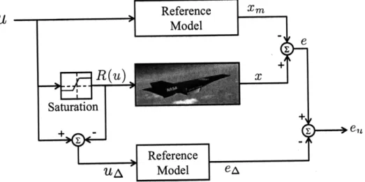
In order to compensate for the modeling uncertainties, an adaptive controller is now added to the baseline controller described in Section 3.2. We note that the adaptive controller is designed so as to directly accommodate for the parametric uncertainties while remaining robust with respect to the unmodeled uncertainties. The structure of the adaptive controller is chosen as

baseline

v = Kffr + K X + (t)Tx (3.20)

nominal adaptive

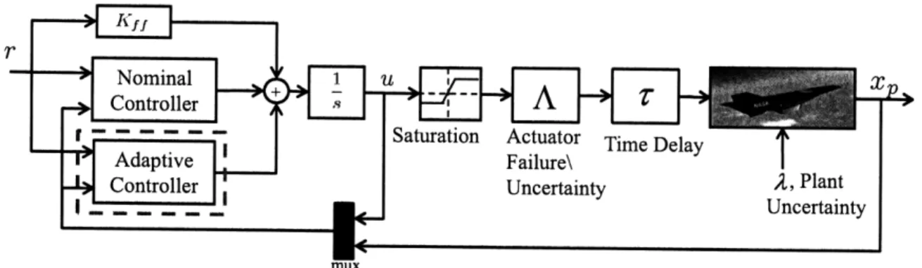
The adaptive component of the controller is denoted, 0, as can be seen in (3.20) and has the same dimension as the nominal feedback gain K. The adaptive component augments naturally with the nominal controller and a visual interpretation of this can be seen in Figure 3-4.

Combining the uncertain plant model in (3.18) with the integral state ej in (3.5), the input-state in (3.6), the the saturation function in (3.19), and the overall baseline

Figure 3-4: Nominal with adaptive augmentation and uncertainty and adaptive control input from (3.20), the closed loop equations are given by,

[1

e =

Ap(A)

H

0

BA

0

x

e

I

L

K1

+

0

(t) K

(t) K3+

(3.21)

where uA = u - _{R,(u), and in compact form reduces to,}

= (A(A, A) + B(K + O(t)T))x + BcmdKffr - BlAuA. (3.22)

A reference model is chosen as

Xm = Amxm - Bmr. (3.23)

where Am and Bm are such that Am is a Hurwitz matrix, Bm = BcmdKff and AAm =

A(A, A) + B(KT + 9*T) - Am is arbitrarily small. We note that due to the addition

parametric uncertainties. Defining the state error e as,

e = x - Xm, (3.24)

we choose adaptive laws for adjusting the adaptive parameter in 3.20 as

= -Foxe PBsign(A) - aoO

U(3.25)

A = -xAdiag(uA)BlPe, - au

where ATP + PAT = -Q and Q = QT > 0. Also eu = e - ea where the auxiliary

error ea is defined as,

ea = Amea - Bldiag(A)uA. (3.26)

The auxiliary error represents the error that occurs do to saturation, and by sub-tracting it from e we obtain a new error e,, which is the uncertainty do to parametric uncertainty and unmodelled dynamics alone. In the above adaptive laws the P's are design parameters that control the rate of adaptation, and the other design param-eter a introduces damping into the laws. The choice of F was driven by an optimal selection function defined in [17] with more details contained in Appendix C.

UJ Reference Xm

Chapter 4

Simulation Studies

In order to assess the robustness of the adaptive control scheme, several simulation studies were performed. In the simulation studies the adaptive controller is compared to the nominal controller under an uncertain plant flight condition. All of the simu-lation begin with the HSV Evaluation Model in level flight at an altitude of 85,000 ft and travelling at Mach 8. The trim values for the HSV at this flight condition are given in Table 4.1.

Table 4.1: Trim values for two input HSV model. State Variable V a q h 0 TIf rif 77a 't a Trim Value 7850 0.0268 0 85000 0.0268 0.939 0 0.775 0

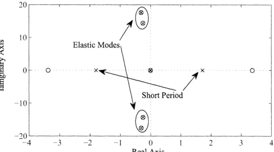
A similar approach to that shown in Equation (3.3) was performed on the Evalu-ation Model. Using the state Jacobian and the input Jacobian matrices a pole-zero plot of the transfer matrix from the control inputs

4

and is shown in Figure 4-1, with a zoom of the origin shown in Figure 4-2. Units ft/s rad rad/s ft rad

Elastic Modes -.-. 0 0 x .. . .. Short Period -. 10 -20 -4 3 -2 - 1 0 1 2 3 4 Real Axis

Figure 4-1: Pole Zero Map for q6,e to Vy.

From the figures it is readily noticed that the HSV has an uncharacteristic short period mode, and is therefore open loop unstable. In most aircraft the short period mode is stable. The HSV lacks this stability because of the slender body and rear controls. The Right Half Plane (RHP) zero arises from the interaction between the elevator deflection, 3_{e, and the heading y. In order for the aircraft to increase the}

euler angle the aircraft must first nose down, so as to gain speed, and then nose up. If this counter intuitive procedure is not carried out and the aircraft is simply brought nose up, then the speed of the aircraft will decrease and the aircraft will begin to loose altitude. Zooming in on the origin of the P-Z map the slow Phugoid mode is found along with a slightly unstable altitude mode.

Eight different sets of simulations are carried out in the this chapter. Four different sets of uncertain plant dynamics will be controlled with both a nominal, non-adaptive, controller and then once with an adaptive controller. The uncertain sets are numbered 1-4 with the non adaptive simulations prefixed with "N" and the adaptive simulation results prefixed with "A". So for example, the first uncertain parameter set simulation with a non-adaptive controller is denoted "NI".

0.05 x " 0Phu oid S"'Altitude -0.05 -1.5 -1 -0.5 0 0.5 1 1.5 Real Axis ,

Figure 4-2: Pole Zero Map zoom in at the origin. in Table 4.2):

1. No uncertainty, nominal plant.

2. Decreased lift and moment coefficients along with the center of gravity moved forward in the HSV. This scenario introduces a more stable aircraft, however decreases the maneuverability of the HSV and will display the control algorithms robustness with respect to saturation.

3. Same as (2) with a significant time delay.

4. Center of gravity moved backwards, leads to more unstable open-loop dynamics as well as increase in the uncertain pitching moment coefficient.

For the simulation studies a filtered step command in altitude of 10,000 ft and a filtered step command of 1,000 ft/s were given. The filter used to generate the smooth commands is that of order two with a damping ratio of 1 and a natural frequency of 0.06 rad. The filtered commands are displayed in Figure 4-3.

The first set of simulations are introduced in order to compare how the adaptive controller compares to the nominal controller when there is no uncertainty. The