Spatial congruence between carbon and biodiversity across forest landscapes of northern Borneo

HAL Id: cirad-01288671

http://hal.cirad.fr/cirad-01288671

Submitted on 16 Mar 2016

HAL is a multi-disciplinary open access

archive for the deposit and dissemination of

sci-entific research documents, whether they are

pub-lished or not. The documents may come from

teaching and research institutions in France or

abroad, or from public or private research centers.

L’archive ouverte pluridisciplinaire HAL, est

destinée au dépôt et à la diffusion de documents

scientifiques de niveau recherche, publiés ou non,

émanant des établissements d’enseignement et de

recherche français ou étrangers, des laboratoires

publics ou privés.

Distributed under a Creative Commons Attribution - NonCommercial - NoDerivatives| 4.0

International License

Spatial congruence between carbon and biodiversity

across forest landscapes of northern Borneo

Nicolas Labrière, Bruno Locatelli, Ghislain Vieilledent, Selly Kharisma, Imam

Basuki, Valéry Gond, Yves Laumonier

To cite this version:

Nicolas Labrière, Bruno Locatelli, Ghislain Vieilledent, Selly Kharisma, Imam Basuki, et al.. Spatial

congruence between carbon and biodiversity across forest landscapes of northern Borneo. Global

Ecology and Conservation, 2016, 6, pp.105-120. �10.1016/j.gecco.2016.01.005�. �cirad-01288671�

Contents lists available atScienceDirect

Global Ecology and Conservation

journal homepage:www.elsevier.com/locate/gecco

Original research article

Spatial congruence between carbon and biodiversity across

forest landscapes of northern Borneo

Nicolas Labrière

a,b,∗

, Bruno Locatelli

a,c

, Ghislain Vieilledent

a

, Selly Kharisma

d

,

Imam Basuki

e

, Valéry Gond

a

, Yves Laumonier

a,d

a_{UPR BSEF, CIRAD (Centre de Coopération Internationale en Recherche Agronomique pour le Développement), Avenue Agropolis,}

34398 Montpellier Cedex 5, France

b_{AgroParisTech, Doctoral School ABIES, 19 Avenue du Maine, 75732 Paris Cedex 15, France} c_{Center for International Forestry Research, Avenida La Molina, 15024 Lima, Peru}

d_{Center for International Forestry Research, Jalan CIFOR, Situ Gede, Sindang Barang, Bogor (Barat) 16115, Indonesia} e_{Oregon State University, Fisheries and Wildlife Department, 2820 SW Campus Way, Corvallis, OR 97331, USA}

h i g h l i g h t s

• We modeled tree diversity and carbon density using field measurements and accessible data.

• Aboveground carbon density and tree diversity were strongly correlated.

• High soil carbon density did not overlap with high aboveground carbon density or tree diversity.

• Protecting areas of high aboveground carbon density will benefit tree diversity.

• High soil carbon in peatlands must be protected with specific regulations.

a r t i c l e i n f o Article history: Received 23 December 2015 Accepted 23 January 2016 Keywords: Ecosystem services Spatialization Spatial relationship REDD+ Protected areas Land-use planning

a b s t r a c t

Understanding how carbon and biodiversity vary across tropical forest landscapes is essential to achieving effective conservation of their respective hotspots in a global context of high deforestation. Whether conservation strategies aimed at protecting carbon hotspots can provide co-benefits for biodiversity protection, and vice versa, highly depends on the extent to which carbon and biodiversity co-occur at the landscape level. We used field measurements and easily accessible explanatory variables to model aboveground carbon density, soil carbon density and tree alpha diversity (response variables) over a mostly forested area of northern Borneo. We assessed the spatial relationships between response variables and the spatial congruence of their hotspots. We found a significant positive relationship between aboveground carbon density and tree alpha diversity, and an above-than-expected-by-chance spatial congruence of their hotspots. Consequently, the protection of areas of high aboveground carbon density through financial mechanisms such as REDD+is expected to benefit tree diversity conservation in the study area. On the other hand, relationships between soil carbon density and both aboveground carbon density and tree alpha diversity were negative and spatial congruences null. Hotspots of soil carbon density, mostly located in peatlands, therefore need specific conservation regulations, which the current moratorium on peat conversion in Indonesia is a first step toward.

© 2016 The Authors. Published by Elsevier B.V. This is an open access article under the CC BY-NC-ND license (http://creativecommons.org/licenses/by-nc-nd/4.0/).

∗_{Corresponding author at: UPR BSEF, CIRAD (Centre de Coopération Internationale en Recherche Agronomique pour le Développement), Avenue}

Agropolis, 34398 Montpellier Cedex 5, France. Tel.: +33 467 593 726; fax: +33 467 593 909.

E-mail address:nicolas.labriere@gmail.com(N. Labrière).

http://dx.doi.org/10.1016/j.gecco.2016.01.005

2351-9894/©2016 The Authors. Published by Elsevier B.V. This is an open access article under the CC BY-NC-ND license (http://creativecommons.org/ licenses/by-nc-nd/4.0/).

1. Introduction

Information on the nature, strength and extent of spatial relationships between multiple ecosystem services (ES) and biodiversity (that can be seen as a good, a final ES or a determinant of the delivery of other ES; seeMace et al., 2012) is crucial for sound ecosystem management and land-use planning (de Groot et al.,2010;Egoh et al.,2008;Naidoo et al., 2008), especially in tropical forest landscapes where conservation versus development goals are at stake (Malhi et al., 2014). Considering multiple ES together constitutes a major challenge in ecosystem management (Raudsepp-Hearne et al., 2010) but is necessary for managing trade-offs between ES and creating new funding opportunities for conservation by bundling co-occurring ES (Carpenter et al.,2006;Wendland et al.,2010).

Tropical forests have long received much attention for conservation, initially with respect to the extraordinary biodiversity that they host (15 of the 25 biodiversity hotspots sensu Myers include tropical forests; seeMyers et al., 2000). The number of tree species in tropical forests, for example, is estimated to lie between 40,000 and 53,000 compared to only 124 tree species across temperate Europe (Slik et al., 2015). To date, the conservation of biodiversity has mostly relied on a network of protected areas. However, the efficiency and effectiveness of this strategy has been challenged because protected areas are too few, too small (at least many of them) and often lack sufficient funding, with only a small fraction of them shown to succeed in disrupting biodiversity erosion (Kramer et al.,1997;Laurance et al.,2012).

In the last decade, the development of REDD

+

, a United Nations initiative aimed at Reducing Emissions from Deforestation and forest Degradation, has shed new light on the necessity to protect tropical forests. Because tropical forests store large amounts of carbon, mostly in living woody biomass (Baccini et al., 2012) and soils (especially in peatlands; see Page et al., 2011), and are currently disappearing fast (Kim et al., 2015), their protection is particularly relevant for climate change mitigation (Pan et al., 2011). The REDD

+

mechanism, which aims to provide financial incentives to maintain and enhance forest carbon stocks, appears to some as an unprecedented opportunity for biodiversity conservation provided strong safeguards are incorporated (Gardner et al.,2012;Paoli et al.,2010;Phelps et al.,2012). However, biodiversity monitoring as part of the social and environmental safeguards for REDD

+

has not received much attention, with the focus clearly remaining on greenhouse gas emission estimations (Dickson and Kapos, 2012).

Schemes dedicated to biodiversity and carbon protection are not meant to be mutually exclusive. Yet many challenges (institutional, political, social, economic, etc.) need to be overcome for protection scheme optimization, for example, protected areas benefiting from the financial support of REDD

+

despite seemingly lack of additionality (a project is ‘additional’ when emission reductions are linked to its implementation and would not have occurred without it;Macdonald et al., 2011), or REDD

+

positively integrating biodiversity safeguards. Beyond scheme design and economic efficiency (that is necessary to tackle the high opportunity cost for conversion and relies for example on incentive structure; e.g. seeBusch et al., 2012;Fisher et al., 2011), whether biodiversity conservation could benefit from climate change mitigation-oriented financial schemes, and vice versa, highly depends on the extent to which carbon and biodiversity co-occur at the landscape level (Strassburg et al., 2010).

So far, there is little agreement on the spatial relationship between carbon storage and biodiversity. At a global scale reports are contradictory, with one study pointing out an ‘‘overall lack of spatial concordance between biodiversity and ecosystem services’’ (including carbon storage; seeNaidoo et al., 2008) while another found a ‘‘high congruence between species richness and biomass carbon’’ (Strassburg et al., 2010). The same seemingly conflicting results arose at national (e.g. seeEgoh et al., 2009vs.Locatelli et al., 2014) and local scales (e.g. seeKessler et al., 2012vs.Ruiz-Jaen and Potvin, 2010).

Three key elements might shed some light on the apparent contradiction between these findings. First, as pointed out by Eigenbrod et al.(2010), proxies used to assess ES distribution may poorly fit primary data, impacting the quality of resulting ES maps and, therefore, the identification of ES hotspots and areas of spatial congruence (i.e. overlap) between multiple ES. Second, the nature, strength and extent of spatial relationships between carbon and biodiversity clearly depend on the metrics selected for carbon (e.g. aboveground carbon only vs. aboveground and soil organic carbon) and biodiversity (e.g. richness, threat, restricted range) in each study (Murray et al., 2015). Third, spatial covariance of ES provision can be influenced by data spatial resolution and study spatial extent (Anderson et al.,2009;Magnago et al.,2015;Murray et al., 2015).

There is a need for more primary data from data-scarce regions to characterize the spatial distribution of, and spatial relationship between, carbon storage and biodiversity so as to guide decision making on land-use planning, especially at the landscape level where most management decisions are made. Working in an area of northern Borneo that is mostly forested but facing clearance with the development of oil palm plantations, we assessed aboveground carbon density (ACD), soil carbon density (SCD, for the 0–20 cm soil layer) and tree alpha diversity (TAD, using Fisher’s

α

) in sampling plots scattered across the study area. The following research questions were addressed: (1) what are the relationships between carbon density and tree diversity across the study area; (2) do carbon and tree diversity hotspots overlap in the study area; and (3) to what extent can biodiversity conservation policies also protect carbon stocks and vice versa. We modeled ACD, SCD and TAD (response variables) with explanatory variables that are easily accessible at the landscape scale. We applied the resulting models over the whole study area and compared our predictions with existing maps for ACD, SCD and TAD. We then explored relationships between response variables and spatial congruence of their respective hotspots. We finally assessed threats and opportunities for carbon storage and tree diversity based on hotspot location, and quantified trade-offs in ES protection from different conservation strategies.

2. Materials and methods

2.1. Study area

Fieldwork was conducted in the Kapuas Hulu regency (hereafter referred to as the ‘‘study area’’) in the Indonesian province of West Kalimantan. The study area spans ca. 31,000 km2of mostly forested land where altitude ranges from 0 to ca. 2000 masl. Mean annual precipitation varies from 2350 to 4300 mm with an average of ca. 3450 mm, and mean annual temperature varies from 17–27°C with an average of ca. 25°C (Hijmans et al., 2005). The majority of soils have developed on sedimentary parent material and belong to the Ultisols, Inceptisols and Histosols orders (RePPProT, 1990).

Two national parks (Betung Kerihun and Danau Sentarum) cover about 30% of the study area (Shantiko et al., 2013). In 2003, Kapuas Hulu was declared a conservation area by the local government, a commitment to improved natural resource management and ecosystem functionality preservation (Prasetyo et al., 2007).

2.2. Field sampling and index computation for carbon and tree diversity

We sampled the main vegetation types between 2011 and 2013. Of the 120 plots sampled, 85 were 100

×

20 m with natural or moderately disturbed vegetation, and 35 were 20

×

20 m with rubber gardens and/or secondary regrowth. Smaller plots were preferred for rubber gardens and secondary regrowth to ensure that plot vegetation was homogeneous despite landscape heterogeneity associated with swidden practices. In each plot, all trees with

≥

10 cm diameter at breast height (1.3 m above ground) were measured, tagged and mapped, and their height estimated using a Blume-Leiss hypsometer (for details, seeWalker et al., 2012). Leaf samples were collected and identified at the Herbarium Bogoriense in Bogor, Indonesia. In total, over the 18.4 ha of surveyed vegetation, 14,155 trees were measured and 4480 herbarium vouchers collected and identified.

Tree dry biomass was computed using a pantropical allometric model that includes tree diameter, tree height and wood specific gravity as explanatory variables (Chave et al., 2014), and carbon content was derived using the standard conversion factor of 0.47 (McGroddy et al., 2004). Wood specific gravity, a constitutive factor of the aforementioned equation, was obtained from the Global Wood Density Database (Zanne et al., 2009). When species were not found in the database, the genus-level average wood density was used instead. Any unresolved cases (ca. 1% of all specimens) were assigned the value of the mean wood density for tropical Southeast Asia (0

.

57 g cm−3_{; seeChave et al., 2009). ACD (in Mg ha}−1_{) was calculated}

by averaging total plot carbon content over plot area.

For mineral soils, composite soil samples were taken for topsoils (0–20 cm; collected using an auger at four different locations for each composite sample) in half of the vegetation plots. Samples were dried at 105°C and further analyzed for carbon content (using Walkley and Black method; seeLandon, 1984). Topsoil cores were also collected using 100 cm3

sample rings to measure dry bulk density (in g cm−3_{). SCD (in Mg ha}−1_{for the 0–20 cm soil layer) was calculated using}

carbon content and dry bulk density. For peat soils, peat samples were collected for topsoils (0–15 cm) using a 203

.

4 cm3

Russian peat sampler. Samples were dried at 60°C and weighted to measure dry bulk density. They were further analyzed for carbon content using a LECO TruSpec induction furnace C analyzer (followingWarren et al., 2012). As we only had a restricted number of soil samples in peatlands and swamp areas (n

=

8), we also reviewed the literature in search of data of (1) soil carbon density or (2) carbon content and bulk density from sampling points geolocalized in the study area. We were only able to retrieve information about two sampling points from one study (Anshari et al., 2010).

We used Fisher’s

α

as an indicator to characterize TAD. Fisher’s

α

, a parametric index, is relatively independent of sample size and insensitive to the presence of rare species (Colwell,2009;Parmentier et al.,2011). For details about sampling strategy, indices computation, and plot structural and compositional features, see Appendix A. Field estimates of ACD, SCD and tree diversity were compared with existing maps (Saatchi et al., 2011andBaccini et al., 2012for ACD;Wieder et al., 2014for SCD;Slik et al., 2009,Raes et al., 2009; andRaes et al., 2013for TAD; see Appendix B for details).

2.3. Potential explanatory variables to be tested for model building

We chose potential explanatory variables that are commonly used in the literature for this type of modeling and for which spatial data were available over the study area (Table 1). We worked at a 250 m grid cell resolution, which is the spatial resolution of MODIS MOD13Q1 (vegetation indices) and MOD44B (vegetation continuous fields) products. These products have been used widely for spatialization of various ground-measured vegetation-related response variables (e.g. seeNagler et al., 2007;Saatchi et al., 2008). All geographical information was projected using a Universal Transverse Mercator projection (zone 49 N, WSG 84 datum).

The MODIS MOD13Q1-derived vegetation indices (EVI and NDVI) have a temporal resolution of 16 days (23 images/year). We gathered images from 2011, 2012 and 2013 to cover the entire fieldwork period. For both EVI and NDVI, we computed a maximum, mean and standard deviation for each grid cell over the 3-year period (i.e. 3

×

23

=

69 images). The MODIS MOD44B-derived vegetation continuous fields (percent tree cover, percent non-tree vegetation and percent non vegetation) have a temporal resolution of one year. We gathered images from 2011 to 2013 and computed the average value for each of the three vegetation continuous fields.

Table 1 Description of the 20 potential explanatory variables tested for ACD, SCD and TAD model building. Source: [1] Available at https://mrtweb.cr.usgs.gov/ ; [2] Available at http://srtm.csi.cgiar.org/ ; [3] Available at http://www.worldclim.org/ ; [4] Ministry of Forestry; [5] Bakosurtanal (National Coordinator for Survey and Mapping Agency); [6] Balittanah (Indonesian Soil Research Institute). Data origin Source Code Description Unit Spatial resolution Range over study area Range over plot network Example reference MODIS [1] EVIMAX Maximum EVI b ind d 250 m 0.1617–1.0000 0.5549–0.9316 Parmentier et al. ( 2011 ) [1] EVIMEAN Mean EVI ind 250 m 0.0298–0. 6459 0.3567–0.5518 Parmentier et al. ( 2011 ) [1] EVISD Standard deviation EVI ind 250 m 0.0447–0.2090 0.0727–0.1349 [1] NDVIMAX Maximum NDVI c ind 250 m 0.3417–0.9995 0.8868–0.9984 Parmentier et al. ( 2011 ) [1] NDVIMEAN Mean NDVI ind 250 m 0.0471–0. 8810 0.6221–0.8391 Parmentier et al. ( 2011 ) [1] NDVISD Standard deviation NDVI ind 250 m 0.0460–0.3106 0.0850–0.2197 Oindo and Skidmore ( 2002 ) [1] PNTV Percent non tree vegetation % 250 m 0–78 6–40 Asner et al. ( 2014 ) [1] PNV Percent non vegetation % 250 m 1–62 5–15 [1] PTC Percent tree cover % 250 m 1–85 50–81 Hansen et al. ( 2003 ) SRTM a [2] ALT Altitude m 90 m → 250 m 13–1955 40–865 Marshall et al. ( 2012 ) [2] SLOPE Slope % 90 m → 250 m 0.0–48.5 0.1–16.3 Marshall et al. ( 2012 ) WordClim [3] TEMPE Mean annual temperature ° C 1 km → 250 m 17.2–26.8 22.5–26.6 Parmentier et al. ( 2011 ) [3] TEMPERANGE Temperature range ° C 1 km → 250 m 8.5–10.0 9.1–9.9 Slik et al. ( 2010 ) [3] TEMPESEAS Temperature seasonality ° C 1 km → 250 m 1.3–4.3 1.9–3.5 Slik et al. ( 2010 ) [3] PRECIP Mean annual precipitation mm 1 km → 250 m 2346–4286 2818–4149 Parmentier et al. ( 2011 ) [3] PRECIPRANGE Precipitation range mm 1 km → 250 m 129–352 190–270 Slik et al. ( 2010 ) [3] PRECIPSEAS Precipitation seasonality mm 1 km → 250 m 15–128 16–38 Slik et al. ( 2010 ) Governmental [4] LANDALLOC Land allocation cat e nr Area for other uses Area for other uses Van der Laan et al. ( 2014 ) Conversion forest Limited production forest Limited production forest National park National park Watershed protectio n forest Production forest Watershed protection forest [5] MINDIST2 Minimum distance to disturbance source (either road, river or village) m nr 0–57,695 0–3579 Van der Laan et al. ( 2014 ) [6] SOIL Soil group cat nr Alluvial Alluvial Slik et al. ( 2009 ) Peat Peat Sedimentary Sedimentary Volcanic Volcanic a SRTM = Shuttle Radar Topographic Mission. b EVI = Enhanced Vegetation Index. c NDVI = Normalized Difference Vegetation Index. d Ind = index, theoretically varying from 0 to 1. e Cat = categorical variable.

Digital elevation data from the NASA Shuttle Radar Topographic Mission were obtained at a 90 m resolution (Jarvis et al., 2008) and further resampled to 250 m. Slope was computed from original data and subsequently resampled to match the designated study resolution.

We also used WorldClim dataset, which provides interpolated estimates of various bioclimatic variables for the 1950–2000 period with a 30 arc-second resolution (

∼

1 km resolution at the equator; seeHijmans et al., 2005), and from which we extracted mean annual temperature, temperature seasonality, temperature range, mean annual precipitation, precipitation seasonality and precipitation range (all resampled to match our 250 m resolution).

Using ArcGis 10, we computed euclidean distances from three potential disturbance sources: roads (including logging roads), rivers and villages. A raster of minimum distance to potential disturbance source was created by selecting the minimum value between the three potential disturbance sources for each grid cell. Land allocation (i.e. the designated use of an area, e.g. production forest or national park) and soil data were also considered potential explanatory variables (obtained from the Ministry of Forestry and the Indonesian Soil Research Institute, respectively; seeTable 1for respective classes).

2.4. Explanatory variable selection and model building

We used ‘‘random forest’’ (a machine learning algorithm; seeBreiman et al., 1984) for explanatory variable selection and response variable modeling. Random forests are collections of decision trees, each trained on a bootstrap sample of a full set of observations. Model accuracy is then evaluated for each tree using observations that had been left out of the corresponding bootstrap sample (Breiman et al., 1984). This modeling technique has already been used to predict aboveground biomass (e.g.Baccini et al., 2012) and tree alpha diversity (e.g.Parmentier et al., 2011).

In case several measurement plots belonged to the same 250 m grid cell, mean response variable values were computed. Sample size was reduced from 120 individual plots to 65 composite sample sites, these constituting our ‘‘full set of observations’’. For each response variable, we grew a random forest of 1000 trees with the 20 potential explanatory variables. We then selected variables based on variable minimal depth and importance value (information available as model outputs; seeIshwaran and Kogalur, 2015). In addition, we eliminated the variables that showed unexplainable partial dependence behavior or whose distribution in observations was not representative of the entire study area. Details about random forest regression algorithm and explanatory variable selection are given in Appendix C.

Once explanatory variables were selected, new 1000-tree random forests were grown for each response variable and their performances in predicting dataset response values recorded. Random forests were finally used to predict response values over the whole study area. Because our measurements focused on tree-dominated vegetation lower than 900 masl, we excluded grid cells with either: (1) water, (2) non-forest vegetation (MODIS percent tree cover

<

50%; followingWaring et al., 2006), or (3) altitude

>

900 m. After mask application, 391,523 grid cells remained.

2.5. Relationships between response variables, spatial congruence of their hotspots and potential threat analysis

We used spatial regression models to study relationships between pairs of response variables based on our predictions. Soil type (mineral vs. peat) was explicitly incorporated in our models to test its influence on relationships between pairs of response variables. Analyses were performed at three different spatial resolutions (250 m, 1 km and 10 km) on a random subset of values (n

=

250, i.e. ca. total number of non-empty grid cells at the coarsest resolution). At 1 km and 10 km spatial resolution, values were drawn among aggregated grid cells for which at least half initial grid cells had values. Analyses were done on original, square root- or log-transformed values, whichever format led to data distribution closest to normality. We tested for spatial autocorrelation on both initial values and residuals of a linear model using Moran’s I. In case residuals were still spatially correlated, we used the Lagrange Multiplier diagnostics for spatial dependence to determine the structure of the appropriate spatial regression model (i.e., spatial error model that accounts for error term correlation vs. spatial lag model that accounts for non-independence between observations;Haining, 1990).

Signs and significance of the resulting model coefficients were used to assess relationships between pairs of response variables. Only results at 250 m spatial resolution are presented here (see Appendix D for results at 1 km and 10 km spatial resolution).

The same method was used to study relationships between our predictions and those from existing maps, except soil type was not incorporated and we only worked at the spatial resolution of existing maps (see Appendix E for details).

For each response variable, hotspots were defined with three different thresholds, as the 10%, 20% or 30% grid cells with highest values. Spatial congruence between hotspots of response variables X and Y was evaluated using the proportion of grid cells that were hotspots for both response variables. This proportion can theoretically vary from 0% to 10% (20% or 30% for other hotspot thresholds, respectively) and would be 1% (4% or 9%, respectively) for two random distributions. The level of spatial congruence was used to infer the potential effect of conservation prioritization (i.e. spatial targeting of conservation measures to hotspots of a given response variable) on non-target response variables. Prioritizing hotspots of the response variable X for conservation was declared beneficial, neutral or detrimental to the non-target response variable Y when spatial congruence was higher, similar or lower than that found between two random distributions (i.e. 1%, 4% or 9% depending on threshold). We worked at a 10 km spatial resolution (i.e. the coarsest spatial resolution of existing maps) to jointly assess the spatial congruence of hotspots of response variables from our predictions and those

Table 2

Selected explanatory variables and random forest performance. 1000-tree random forests were grown for each response variable. The number of variables tried at each split was consistently 1 (default value: total number of explanatory variables/3).

Response variable Explanatory variables MSRa _RMSRb _{Variance explained (%)}

ACD PTC+ALT 2302.4 48.0 75.7 SCD ALT+TEMPE+SOIL 2049.0 45.3 52.4 TAD ALT+TEMPESEAS+TEMPE+PTC 110.8 10.5 77.9

a_{MSR=mean of squared residuals.} b_{RMSR=root mean of squared residuals.}

of existing maps. Only results using the 10% threshold are presented here (see Appendix F for results using the 20% and 30% thresholds).

To assess potential threats to hotspots of response variables over the study area, we classified hotspot grid cells according to the land allocation under which they are situated, and recorded whether the corresponding areas were included in logging, mining or plantation concessions (concession data obtained from the Ministry of Forestry). We only performed this potential threat analysis on our predictions and therefore worked at the original (i.e. 250 m) spatial resolution of our predictions.

All statistical analyses were done using R (R Core Team, 2014). Most frequently used R packages include ‘vegan’ (Oksanen et al., 2015), ‘raster’ (Hijmans, 2015), ‘spdep’ (Bivand and Piras, 2015;Bivand et al.,2013), ‘randomForest’ (Liaw and Wiener, 2002) and ‘randomForestSRC’ (Ishwaran and Kogalur, 2015).

3. Results

3.1. Response variable predictions over the study area

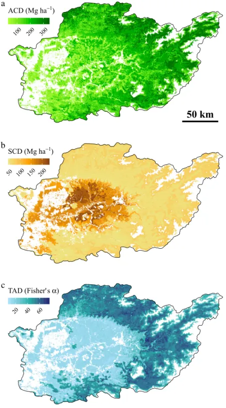
Altitude was a key explanatory variable for all response variables, whereas percent tree cover was only important in explaining ACD and TAD (Fig. 1,Table 2). The percentage of variance explained by the models ranged from 50%–80% depending on response variable. Application of these models over the study area revealed differences in the broad pattern of response variable distribution, with high spatial variability for ACD, and the highest values for TAD and SCD in the outer and inner part of the study area, respectively (Fig. 2).

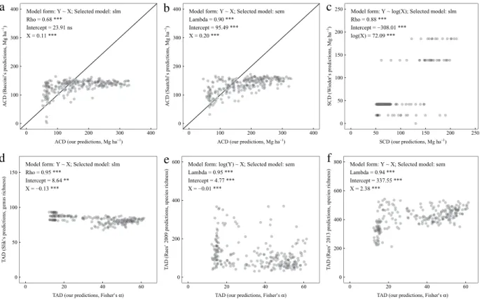
Our predictions of all response variables were significantly correlated to their values in existing maps but the fit was often poor (Fig. 3). When comparing our predictions of ACD with those of existing maps, we found that the slope was only a tenth to a fifth that of the slope expected in case of perfect match. We also evidenced a saturation effect from both existing maps (i.e. none to few of their predicted values exceeded a threshold of about 175 Mg ha−1;Fig. 3(a)–(b)). There was a significant positive relationship between our predictions of SCD and the top 30 cm soil carbon values in the Harmonized World Soil Database despite the limited number of unique values of the latter (Fig. 3(c)). Comparisons of our predictions of TAD with three existing maps showed mixed results, with relationships being either negative or positive depending on which map was used (seeFig. 3(d)–(f)).

3.2. Response variable relationships and hotspot spatial congruence

Despite soil type (mineral vs. peat) being consistently tested for inclusion in the models, the most parsimonious models did not necessarily include soil type and/or its interaction with other predictors (Table 3). The relationship between TAD and ACD was positive and the interaction between ACD and soil type – but not soil type itself – was significant and negative. In other words, TAD increased more rapidly with increasing ACD over mineral soils than over peat soils. Neither soil type nor its interaction with SCD was a significant predictor of TAD, and we found that TAD significantly decreased with increasing SCD. Soil type and SCD were both significant predictors of ACD, the latter being higher over peat soils for a given SCD and decreasing with increasing SCD. Analyzing the same relationships at 1 km and 10 km spatial resolution, we did not find any strong scale-dependent effects on our findings (see Appendix D).

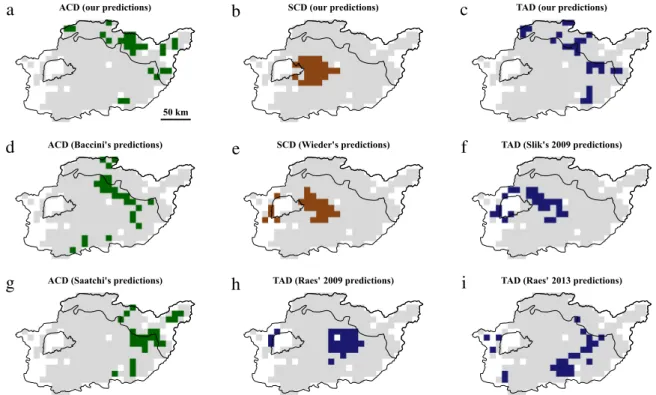
Spatial congruence was very variable depending on the nature (ACD, SCD or TAD) and source (our predictions vs. predictions from existing maps) of response variables under consideration except for spatial congruence between hotspots of ACD and SCD that was consistently null (Fig. 4,Table 4). We found no spatial congruence between hotspots of SCD and TAD based on our predictions while spatial congruence could potentially be high based on predictions from some other sources, e.g. for SCD (Wieder’s) with TAD (Slik’s). According to our predictions, spatial congruence between hotspots of ACD and TAD was more than three times (3.5:1) higher than expected if hotspot spatial distributions were random, meaning that about a third of ACD hotspots were also hotspots of tree diversity. Conversely, most combinations of predictions of ACD and TAD resulted in spatial congruence null or close to that attained for random distributions. Using 20% or 30% thresholds for hotspot definition did not lead to markedly different results on spatial congruence between hotspots of ACD, SCD and TAD (see Appendix F).

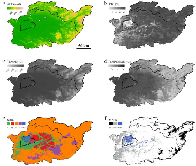
Fig. 1. Spatial representation of explanatory variables selected for response variable prediction: (a) altitude, (b) percent tree cover, (c) mean annual

temperature, (d) temperature seasonality and (e) soil type (AL=alluvial; PE=peat; SE=sedimentary; VO=volcanic; WA=water). Areas depicted in (f) are those where masks were applied (ALT=altitude>900 m; NFO=non-forest area; WAT=water). Areas where field surveys were conducted are indicated by white dots in (a). The two national parks present in Kapuas Hulu (Betung Kerihun and Danau Sentarum, N-E and W part of the study area, respectively) are also displayed.

4. Discussion

4.1. Ecological insight about the relationship between ACD and TAD

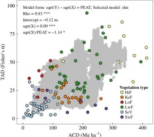
We found a significant positive relationship between our predictions of ACD and TAD over the study area. The only non-null spatial congruence – at least when considering our predictions – was found between hotspots of ACD and TAD. Using values computed from field measurements (those from which our predictions originated), we found a significant positive relationship between ACD and TAD (Fig. 5) despite high ACD variability for a given TAD value.

Part of that variability is inherently due to that we surveyed very different vegetation types. For example, TAD could be similar for some lowland natural forest and peat swamp plots (e.g. Fisher’s

α =

25; seeFig. 5), but ACD was much lower in the latter vegetation type. Soil nutrient content has been shown to affect spatial variations of aboveground biomass (and therefore carbon density) and tree diversity in Borneo (Cannon and Leighton, 2004;Paoli et al.,2008), with forests growing on oligotrophic soils (e.g. Kerangas forests on sandstone and peat swamp forests) containing lower aboveground biomass and fewer tree species than nearby forests on well-drained mineral soils (e.g. seeAnderson, 1964andBrünig, 1974). While we found that TAD was limited in most nutrient-poor natural forest plots, ACD was more variable and some values reached surprisingly high levels compared to those of lowland natural forest plots on mineral soils (seeFig. 5). This potentially originates from the relatively small size of our plots (0.04–0.2 ha).

Fig. 2. Map of predicted response variables over the study area: (a) aboveground carbon density (ACD), (b) soil carbon density (SCD), (c) tree alpha diversity

(TAD, using Fisher’sα). White areas correspond to areas where masks were applied.

Two – not necessarily mutually exclusive – hypotheses have gained attention in explaining how biodiversity might influence ecosystem properties such as carbon storage. The niche complementarity hypothesis states that higher levels of biodiversity lead to greater carbon storage because of increased resource use, whereas the mass ratio hypothesis holds that carbon storage is mostly driven by functional trait properties of the dominant species (Loreau and Hector, 2001). The significant positive relationship we found between ACD and TAD supports the niche complementarity hypothesis. Consistent with our findings, a study conducted in Panama found that species richness increased tree carbon storage (Ruiz-Jaen and

Fig. 3. Comparison of our predictions with values extracted from existing maps of (a) ACD (Baccini et al., 2012); (b) ACD (Saatchi et al., 2011); (c) SCD (Wieder et al., 2014); (d) TAD (Slik et al., 2009); (e) TAD (Raes et al., 2009); (f) TAD (Raes et al., 2013). Information about the best-fit significant model (selected among linear and spatial regression models) is displayed in each facet. Model coefficients (for spatial dependence and/or intercept and independent variable) are presented along with information on statistical significance. Variable: ACD = aboveground carbon density; SCD =soil carbon density; TAD = tree alpha diversity; Selected model: lm = linear model; slm = spatial lag model; Significance: n.s. non-significant;∗

p< 0.05;

∗∗

p<0.01;∗∗∗ p<0.001.

Table 3

Relationships between ACD, SCD and TAD (response variables) over the study area depending on soil type (mineral vs. peat). Analyses were performed on a random subset of response variable values (n=250) from our predictions at 250 m spatial resolution. We used original, square root- or log-transformed data, whichever format led to data distribution closest to normality. Depicted values are either test statistics (for Moran’s I, Lagrange Multiplier and the selected model) or model coefficients, and are presented along with information on statistical significance. Note that the most parsimonious model did not necessarily include soil type and/or its interaction.

General model form Y∼X∗PEAT

Model 1 Model 2 Model 3

Variablea _{Y=TAD X=ACD Y=TAD X=SCD Y=ACD X=SCD}

Data format Sqrt Sqrt Original log+1 Original log+1 Moran’s I On variable 0.26 ∗∗∗ 0.19∗∗∗ 0.21∗∗∗ 0.13∗∗∗ 0.23∗∗∗ 0.18∗∗∗

On linear model residuals 0.07∗∗∗ _0.16∗∗∗ _0.17∗∗∗

Lagrange Multiplier (LM) LMerr 40.20

∗∗∗

282.74∗∗∗

272.17∗∗∗

LMlag 70.46∗∗∗ 355.24∗∗∗ 335.38∗∗∗

Selected model typeb _{slm slm slm}

Model statisticc _583.05∗∗∗ 3030.37∗∗∗ 2466.41∗∗∗ Model coefficients Intercept −2.96∗∗∗ 84.91∗∗∗ 252.37∗∗∗ X 0.26∗∗∗ ₋ 19.40∗∗∗ ₋ 57.75∗∗∗ PEAT 1.36 ns – 43.00∗∗ X:PEAT −0.20∗∗ – – Spatial dependenced _0.94∗∗∗ 0.97∗∗∗ 0.97∗∗∗

a_{Variable: ACD= aboveground carbon density; SCD=soil carbon density; TAD=tree alpha diversity; PEAT=binary variable with mineral=0}

and peat=1.

b _{sem=spatial error model; slm=spatial lag model.} c _{Wald statistic for spatial error or spatial lag model.}

d _{Rho in case of spatial lag model, Lambda in case of spatial error model.}

n.s. non-significant;∗∗

p<0.01;∗∗∗

p<0.001.

Potvin, 2010). However, the study also showed that dominance was important in explaining tree carbon storage variations, thus highlighting the relevance of the mass ratio hypothesis. More work is required to test the mass ratio hypothesis with

Fig. 4. Spatial distribution of hotspots of response variables at 10 km spatial resolution using a 10% threshold: (a) ACD (our predictions); (b) SCD (our

predictions); (c) TAD (our predictions); (d) ACD (Baccini et al., 2012); (e) SCD (Wieder et al., 2014); (f) TAD (Slik et al., 2009); (g) ACD (Saatchi et al., 2011); (h) TAD (Raes et al., 2009); (i) TAD (Raes et al., 2013).

Table 4

Spatial congruence between hotspots of ACD, SCD and TAD (response variables) at 10 km spatial resolution using a 10% threshold. Values (percentage of overlapping grid cells over the total number of grid cells) potentially range from 0 to 10%. Expected spatial congruence for two variables with random spatial distribution is 1%. For the sake of readability, values are highlighted with different colors depending on the nature of the response variables under consideration (yellow, green and blue for ACD-SCD, ACD-TAD and SCD-TAD, respectively).

regard to our data and to weight, if necessary, the relative relevance of the two hypotheses in such a tropical forest context. Analyzing the compositional component of tree diversity and species turnover from site to site might also help gain new insights into ecosystem functioning and subsequent carbon storage.

4.2. Potential threats over carbon and tree diversity hotspots

Considering land allocation as an indicator of potential threats to carbon and tree diversity hotspots, we found that a very high proportion of ACD and TAD hotspots were located either in watershed protection forests or national parks (Table 5). Very few ACD and TAD hotspots were found in concessions, which legally avoid watershed protection forests or national parks (see Appendix G for more information about concessions extent and location). Overall, provided current land allocation is maintained and the law is enforced to ensure the integrity of protected areas, ACD and TAD hotspots appear to be under low threat.

In contrast, we found that a worryingly high proportion of SCD hotspots were located in areas under disturbance-prone land allocation (‘‘area for other uses’’ and ‘‘limited production forest’’) and overlapped logging and/or plantation concessions (Table 5). This raises concerns about the extent to which soil carbon stocks are secured in the study area. The vast majority

Fig. 5. Tree alpha diversity (TAD, using Fisher’sα) against aboveground carbon density (ACD). Gray dots represent model predictions (10% random selection) over the study area. Colored dots correspond to field measurements. Information about the best-fit significant model between TAD and ACD (selected among linear and spatial regression models) is also displayed. Soil type (mineral vs. peat) and its interaction with ACD were tested for inclusion in the model. The most parsimonious model included the interaction term but not soil type itself. Model coefficients (for spatial dependence, intercept, independent variable and interaction between soil type and independent variable) are presented along with information on statistical significance. Vegetation type: HiF= hill natural forest on mineral soil; KeF=Kerangas forest (i.e. forest on sandstone); LoF= logged-over forest; LwF=lowland natural forest on mineral soil; SeV =secondary vegetation (either secondary regrowth or rubber gardens); SwF= swamp forest (either freshwater or peat swamp forests); Selected model: slm=spatial lag model; Significance: n.s. non-significant;∗

p<0.05;∗∗

p<0.01;∗∗∗

p<0.001. (For interpretation of the references to color in this figure legend, the reader is referred to the web version of this article.)

Table 5

Distribution (%) of response variable hotspots depending on land allocation and presence of concession at 250 m spatial resolution using a 10% threshold. The expected repartition of hotspots of a response variable with random distribution is given for comparison. Land allocation columns are ordered from left to right along a gradient of decreasing likeliness of disturbance. The sum of each row across the six land allocation types is equal to 100%. Note that there can be more than one concession type on the same grid cell. A high proportion of SCD hotspots (compared to hotspots of other response variables) are situated in areas that are (most) likely to be disturbed.

Hotspot of response variable

Land allocation Concessions Area for other uses Conversion forest Production forest Limited production forest Watershed protection forest National park

Logging Mining Plantation

Random distribution 24 1 5 17 23 30 10 11 17 ACD <1 0 <1 5 26 69 <1 1 <1

SCD 40 7 6 33 3 11 27 6 21

TAD 1 0 <1 13 37 49 2 3 <1

of SCD hotspots were situated in peatlands. For almost 4 years now, there has been a moratorium on the issuance of new licenses for logging and conversion to other land uses in natural forests and peatlands. Whether the moratorium is effective in reducing the deforestation rate is highly debated (Busch et al.,2015;Sloan et al.,2012). Nevertheless, the concessions we consider here were granted prior to 2012, and designated areas are therefore susceptible to being legally selectively logged and/or cleared at any time.

We did not rank concession types according to their impacts on ecosystems but do acknowledge that all activities are not equally damaging. There is a general consensus about the deleterious effect on biodiversity and ES of forest conversion – especially in peatlands – to monocrop plantations (e.g. seeKoh and Wilcove, 2008;Savilaakso et al., 2014). In comparison, logged-over forests have been shown to maintain relatively high levels of services (Putz et al., 2012) provided harvesting techniques that reduce the negative impact of logging on biodiversity and ES (e.g. ‘reduced-impact logging’ techniques) are used (Edwards et al., 2014).

4.3. Implications for conservation and development

Significant positive relationships between ES do not necessarily imply high spatial congruence between their respective hotspots, and vice versa (Chan et al., 2006). Yet, in our case, we found a significant positive relationship between ACD and TAD, and an above-than-expected-by-chance spatial congruence of hotspots. Prioritizing hotspots of one of ACD or TAD for

conservation would therefore be beneficial to the other (Table 4). However, either type of prioritization would be detrimental to SCD, as would be SCD hotspot targeting for non-target response variables.

The spatial variations in total carbon stocks (i.e. carbon stored in aboveground biomass, belowground biomass, dead wood, litter and soil organic carbon) are mainly determined by variations in soil organic carbon, with stocks in peat forests largely outperforming those of forests on mineral soils (Page et al.,2011;Paoli et al.,2010). If REDD

+

projects only try to maximize total carbon stock protection (i.e. focus on peatlands), additional gains for biodiversity conservation appear limited. We stress that REDD

+

projects should target hotspots of ACD rather than SCD, which would also benefit TAD but would probably not be the most economically competitive option to counter the high opportunity cost for conversion (Fisher et al., 2011). In our case, preferential areas for REDD

+

project development are in conservation areas or watershed protection forests. Yet, directing REDD

+

funds toward conservation areas such as national parks is still controversial because of the seemingly lack of additionality (Macdonald et al., 2011). Gaining effective protection through the use of REDD

+

funds would nonetheless de facto constitute additionality for those of the national parks where protection is currently missing (the so-called ‘‘paper parks’’). Until the institutional framework is clarified, targeting high-ACD watershed protection forests that are adjacent to national parks for REDD

+

project development could be a first step in hindering the general trend of national park isolation that has been increasing for the last few decades (DeFries et al., 2005).

SCD hotspot protection, on the other hand, could be achieved through the strict enforcement of the current moratorium that has been praised, despite other caveats, as succeeding in peatland protection (Edwards et al.,2012;Sloan et al.,2012). Re-evaluation of permits delivered prior to 2012, especially for mining and plantations that would lead to permanent conversion of peatlands, could provide further benefits to SCD hotspot protection. If old concessions on peatlands were re-allocated, logged-over forests on mineral soils should undoubtedly be spared and allowed to recover as they provide ES similar to those of natural forests (Labrière et al.,2015;Meijaard and Sheil, 2007). Development of plantation concessions should be directed to highly degraded lowland areas on mineral soils. Some plantation concessions (e.g. timber plantations) could even lead to ecological benefits beyond economic ones (Lamb et al., 2005). Plantations of the exotic species Acacia

mangium have, for example, been used successfully to restore natural vegetation in degraded Imperata cylindrica grasslands

(Kuusipalo et al., 1995).

The future role of oil palm plantations (the vast majority of plantation concessions granted before 2012) in the development of Kapuas Hulu cannot be overlooked. As the extent of oil palm plantations is predicted to triple in Kalimantan by 2020 (Carlson et al., 2013), it is essential that oil palm establishment is carefully planned and plantations well managed, two conditions necessary for plantations to provide not only goods but also services to a certain extent (Sayer et al., 2012). Plantations developed only on highly degraded lands and incorporated within a matrix of land uses related to the traditional swidden system (that produce more services than oil palm plantations; see e.g.Labrière et al., 2015) could allow for development in Kapuas Hulu that would not be detrimental to carbon and biodiversity conservation. However, sound development options will be limited due to the peculiar biophysical characteristics of the area (steep slopes and peats in the outer and inner parts of the study area, respectively) that restrict the range of potential non-harmful human activities.

4.4. Limitations of our predictions and those from existing maps, and perspectives on spatial congruence analysis

Despite the fact that we used the best available data, the main limitations of our predictions arise from: (1) the still restricted size of our measurement dataset, and (2) the reliability of explanatory variable data. We tried to sample at least 2 ha per main vegetation type while an inventory of 4–6 ha would for instance be recommended to assess biomass of the lowland and hill dipterocarp forests of Indonesia with an error margin not higher than 6%–8% (Laumonier et al., 2010). More vegetation and soil sampling will be required to challenge our predictions and gain a better knowledge of carbon and tree species distribution over the study area. Our predictions also depend on the choice and reliability of explanatory variable data. Though allowing for discrimination between open canopy disturbed forest and closed-canopy natural forests, percent tree cover (selected as explanatory variable in ACD and TAD models) alone would probably fail at capturing biomass variations between different forest types of equally high percent tree cover (Houghton et al., 2001). Yet, other variables included in the model, such as altitude, would have served as surrogates for forest type discrimination. WorldClim data, for example, are obtained by interpolating measurements collected over a vast network of weather stations worldwide. Yet, the density of weather stations was extremely low in our study area and over Borneo more generally (Hijmans et al., 2005). The nature of relationships between our predictions and those from existing maps was highly variable. While significant positive relationships were found between our ACD predictions and those fromSaatchi et al.(2011) andBaccini et al.(2012), we found a clear saturation of their predictions (seeFig. 3). Several studies recently challenged the accuracy of predictions from those maps, arguing that they fail to capture some forest carbon patterns both at regional (Mitchard et al., 2014) or pantropical (Avitabile et al., 2015) scale. The saturation effect might be due to poor performance of GLAS (the Geoscience Laser Altimeter System) height estimation in hilly terrain with slope over 10°–15°(about a third of our study area;Hilbert and Schmullius, 2012), asymptotical saturation of NDVI values in high biomass regions (Huete et al., 2002) and limited field sampling in Southeast Asian tropical forests that are structurally different from those of America and Africa (Slik et al., 2013). While significant negative relationships were found between our predictions of TAD and those fromSlik et al.(2009) andRaes et al.(2009), more recent predictions fromRaes et al.(2013) are better aligned with ours. Species distribution models used inRaes et al.(2013) were obtained from a larger database of collection records and did not suffer from partial distribution modeling (Raes, 2012), as in earlier predictions.

While hotspot-based approaches are widely used to study spatial congruence between ecosystem services (e.g. see Egoh et al., 2008;Eigenbrod et al., 2010;Locatelli et al., 2014), such approaches might face limitations regarding spatial conservation prioritization. Conversely, the use of alternative tools such as Marxan (Ball et al., 2009) or Zonation (Moilanen et al., 2005), which allow for acquisition cost inclusion and fragmentation limitation for spatial conservation prioritization, has already proved valuable in helping identifying priority areas for joint biodiversity and ES conservation (e.g. seeChan et al., 2006andThomas et al., 2013) but exceeded the scope of our biophysical characterization of ES distribution in a data-scarce region. Further research could explore landscape and socioeconomic scenarios, using information about administratively meaningful planning units (e.g. districts or villages), tenure status, designated land allocation and the opportunity cost of conservation.

5. Conclusion

Mapping the distribution of biodiversity and ecosystem services is crucial to guide decision making on land-use planning. Using field measurements and easily accessible explanatory variables, we were able to predict aboveground carbon density, soil carbon density and tree alpha diversity (response variables) over a mostly forested area of northern Borneo. Analyses of the relationships between response variables, and the spatial congruence of and potential threats to their respective hotspots, enabled us to discuss implications of carbon and tree diversity spatial distributions for conservation and development. We stress that prioritizing hotspots of aboveground carbon – and not total carbon – for conservation through financial mechanisms such as REDD

+

would be beneficial for tree diversity conservation in the study area even if it might not be the most economically competitive option to counter the high opportunity cost for conversion. The protection of the large carbon pool in peat soils should be achieved by conservation regulations, which the current moratorium on peat conversion in Indonesia is a first step toward. Re-allocating plantation concessions on highly degraded areas could help achieve economic development (and also ecosystem restoration in the case of timber plantations) in Kapuas Hulu without imperiling carbon and biodiversity conservation.

We believe that our approach can be used to predict the spatial distribution of other important ecosystem services in Kapuas Hulu (e.g. water flow regulation) or be transposed in other areas for the purpose of reaching an integrated ecosystem service based approach for land-use planning (Daily and Matson, 2008).

Acknowledgments

We are deeply grateful to villagers from Keluin, Nanga Dua, Belatong, Banua Tengah and Nanga Hovat for their hospitality and help in data collection. We warmly thank Bapak Engkamat for his precious help and support during fieldwork. We are thankful to Bapak Bundani from Polisi Kehutanan who joined the team and helped during surveys conducted in the Betung Kerihun National Park. We are much indebted to Bapak Ismail Rachman from the Herbarium Bogoriense for voucher identification. We are also sincerely grateful to Niels Raes and Ferry Slik for sharing data from previous work. This research received financial support from CIRAD, CoLUPSIA (EU financed project DCI), AusAid (Agreement 63650 with Center for International Forestry Research), ABIES (Ecole Doctorale Agriculture, Alimentation, Biologie, Environnements et Santé) and CRP-FTA (Consortium Research Program on Forests, Trees, and Agroforestry).

Appendix A. Supplementary data

Supplementary material related to this article can be found online athttp://dx.doi.org/10.1016/j.gecco.2016.01.005.

References

Anderson, J.A.R.,1964. The structure and development of the peat swamps of Sarawak and Brunei. J. Trop. Geogr. 18, 7–16.

Anderson, B.J., Armsworth, P.R., Eigenbrod, F., Thomas, C.D., Gillings, S., Heinemeyer, A., Roy, D.B., Gaston, K.J., 2009. Spatial covariance between biodiversity and other ecosystem service priorities. J. Appl. Ecol. 46, 888–896.http://dx.doi.org/10.1111/j.1365-2664.2009.01666.x.

Anshari, G., Afifudin, M., Nuriman, M., Gusmayanti, E., Arianie, L., Susana, R., Nusantara, R., Sugardjito, J., Rafiastanto, A.,2010. Drainage and land use impacts on changes in selected peat properties and peat degradation in West Kalimantan Province, Indonesia. Biogeosciences 7, 3403–3419.

Asner, G.P., Knapp, D.E., Martin, R.E., Tupayachi, R., Anderson, C.B., Mascaro, J., Sinca, F., Chadwick, K.D., Higgins, M., Farfan, W., Llactayo, W., Silman, M.R., 2014. Targeted carbon conservation at national scales with high-resolution monitoring. Proc. Natl. Acad. Sci. USA 111, E5016–E5022.

http://dx.doi.org/10.1073/pnas.1419550111.

Avitabile, V., Herold, M., Heuvelink, G.B.M., Lewis, S.L., Phillips, O.L., Asner, G.P., Armston, J., Asthon, P., Banin, L.F., Bayol, N., Berry, N., Boeckx, P., de Jong, B., DeVries, B., Girardin, C., Kearsley, E., Lindsell, J.A., Lopez-Gonzalez, G., Lucas, R., Malhi, Y., Morel, A., Mitchard, E., Nagy, L., Qie, L., Quinones, M., Ryan, C.M., Slik, F., Sunderland, T., Vaglio Laurin, G., Valentini, R., Verbeeck, H., Wijaya, A., Willcock, S., 2015. An integrated pan-tropical biomass map using multiple reference datasets. Global Change Biol.http://dx.doi.org/10.1111/gcb.13139.

Baccini, A., Goetz, S.J., Walker, W.S., Laporte, N.T., Sun, M., Sulla-Menashe, D., Hackler, J., Beck, P.S.A., Dubayah, R., Friedl, M.A., Samanta, S., Houghton, R.A., 2012. Estimated carbon dioxide emissions from tropical deforestation improved by carbon-density maps. Nature Clim. Change 2, 182–185.

http://dx.doi.org/10.1038/Nclimate1354.

Ball, I.R., Possingham, H.P., Watts, M.,2009. Marxan and relatives: software for spatial conservation prioritisation. In: Moilanen, A., Wilson, K.A., Possingham, H.P. (Eds.), Spatial Conservation Prioritisation: Quantitative Methods and Computational Tools. Oxford University Press, Oxford, pp. 185–195.

Bivand, R.S., Hauke, J., Kossowski, T.,2013. Computing the Jacobian in Gaussian spatial autoregressive models: An illustrated comparison of available methods. Geogr. Anal. 45, 150–179.

Bivand, R., Piras, G.,2015. Comparing implementations of estimation methods for spatial econometrics. J. Stat. Softw. 63, 1–36.

Breiman, L., Friedman, J., Stone, C.J., Olshen, R.A.,1984. Classification and Regression Trees. CRC Press, Belmont, CA.

Brünig, E.F., 1974. Ecological studies in the kerangas forests of Sarawak and Brunei. Borneo Literature Bureau for Sarawak Forest Department.

Busch, J., Ferretti-Gallon, K., Engelmann, J., Wright, M., Austin, K.G., Stolle, F., Turubanova, S., Potapov, P.V., Margono, B., Hansen, M.C., Baccini, A., 2015. Reductions in emissions from deforestation from Indonesia’s moratorium on new oil palm, timber, and logging concessions. Proc. Natl. Acad. Sci. USA 112, 1328–1333.http://dx.doi.org/10.1073/pnas.1412514112.

Busch, J., Lubowski, R.N., Godoy, F., Steininger, M., Yusuf, A.A., Austin, K., Hewson, J., Juhn, D., Farid, M., Boltz, F., 2012. Structuring economic incentives to reduce emissions from deforestation within Indonesia. Proc. Natl. Acad. Sci. 109, 1062–1067.http://dx.doi.org/10.1073/pnas.1109034109.

Cannon, C.H., Leighton, M., 2004. Tree species distributions across five habitats in a Bornean rain forest. J. Veg. Sci. 15, 257–266.

http://dx.doi.org/10.1111/j.1654-1103.2004.tb02260.x.

Carlson, K.M., Curran, L.M., Asner, G.P., Pittman, A.M., Trigg, S.N., Adeney, J.M., 2013. Carbon emissions from forest conversion by Kalimantan oil palm plantations. Nature Clim. Change 3, 283–287.http://dx.doi.org/10.1038/nclimate1702.

Carpenter, S.R., DeFries, R., Dietz, T., Mooney, H.A., Polasky, S., Reid, W.V., Scholes, R.J., 2006. Millennium ecosystem assessment: Research needs. Science 314, 257–258.http://dx.doi.org/10.1126/science.1131946.

Chan, K.M., Shaw, M.R., Cameron, D.R., Underwood, E.C., Daily, G.C., 2006. Conservation planning for ecosystem services. PLoS Biol. 4, 2138–2152.

http://dx.doi.org/10.1371/journal.pbio.0040379.

Chave, J., Coomes, D., Jansen, S., Lewis, S.L., Swenson, N.G., Zanne, A.E., 2009. Towards a worldwide wood economics spectrum. Ecol. Lett. 12, 351–366.

http://dx.doi.org/10.1111/j.1461-0248.2009.01285.x.

Chave, J., Réjou-Méchain, M., Búrquez, A., Chidumayo, E., Colgan, M.S., Delitti, W.B.C., Duque, A., Eid, T., Fearnside, P.M., Goodman, R.C., Henry, M., Martínez-Yrízar, A., Mugasha, W.A., Muller-Landau, H.C., Mencuccini, M., Nelson, B.W., Ngomanda, A., Nogueira, E.M., Ortiz-Malavassi, E., Pélissier, R., Ploton, P., Ryan, C.M., Saldarriaga, J.G., Vieilledent, G., 2014. Improved allometric models to estimate the aboveground biomass of tropical trees. Global Change Biol. 20, 3177–3190.http://dx.doi.org/10.1111/gcb.12629.

Colwell, R.K.,2009. Biodiversity: concepts, patterns, and measurement. In: Levin, S.A. (Ed.), The Princeton Guide to Ecology. Princeton University Press, Princeton, NJ, pp. 257–263.

Daily, G.C., Matson, P.A., 2008. Ecosystem services: From theory to implementation. Proc. Natl. Acad. Sci. 105, 9455–9456.

http://dx.doi.org/10.1073/pnas.0804960105.

de Groot, R.S., Alkemade, R., Braat, L., Hein, L., Willemen, L., 2010. Challenges in integrating the concept of ecosystem services and values in landscape planning, management and decision making. Ecol. Complex. 7, 260–272.http://dx.doi.org/10.1016/j.ecocom.2009.10.006.

DeFries, R., Hansen, A., Newton, A.C., Hansen, M.C., 2005. Increasing isolation of protected areas in tropical forests over the past twenty years. Ecol. Appl. 15, 19–26.http://dx.doi.org/10.1890/03-5258.

Dickson, B., Kapos, V., 2012. Biodiversity monitoring for REDD+. Curr. Opin. Environ. Sustain. 4, 717–725.http://dx.doi.org/10.1016/j.cosust.2012.09.017. Edwards, D.P., Koh, L.P., Laurance, W.F., 2012. Indonesia’s REDD+ pact: Saving imperilled forests or business as usual? Biol. Cons. 151, 41–44.

http://dx.doi.org/10.1016/j.biocon.2011.10.028.

Edwards, D.P., Tobias, J.A., Sheil, D., Meijaard, E., Laurance, W.F., 2014. Maintaining ecosystem function and services in logged tropical forests. Trends Ecol. Evol. 29, 511–520.http://dx.doi.org/10.1016/j.tree.2014.07.003.

Egoh, B., Reyers, B., Rouget, M., Bode, M., Richardson, D.M., 2009. Spatial congruence between biodiversity and ecosystem services in South Africa. Biol. Cons. 142, 553–562.http://dx.doi.org/10.1016/j.biocon.2008.11.009.

Egoh, B., Reyers, B., Rouget, M., Richardson, D.M., Le Maitre, D.C., van Jaarsveld, A.S., 2008. Mapping ecosystem services for planning and management. Agric. Ecosyst. Environ. 127, 135–140.http://dx.doi.org/10.1016/j.agee.2008.03.013.

Eigenbrod, F., Armsworth, P.R., Anderson, B.J., Heinemeyer, A., Gillings, S., Roy, D.B., Thomas, C.D., Gaston, K.J., 2010. The impact of proxy-based methods on mapping the distribution of ecosystem services. J. Appl. Ecol. 47, 377–385.http://dx.doi.org/10.1111/j.1365-2664.2010.01777.x.

Fisher, B., Edwards, D.P., Giam, X., Wilcove, D.S.,2011. The high costs of conserving Southeast Asia’s lowland rainforests. Front. Ecol. Environ. 9, 329–334.

Gardner, T.A., Burgess, N.D., Aguilar-Amuchastegui, N., Barlow, J., Berenguer, E., Clements, T., Danielsen, F., Ferreira, J., Foden, W., Kapos, V., Khan, S.M., Lees, A.C., Parry, L., Roman-Cuesta, R.M., Schmitt, C.B., Strange, N., Theilade, I., Vieira, I.C.G., 2012. A framework for integrating biodiversity concerns into national REDD+programmes. Biol. Cons. 154, 61–71.http://dx.doi.org/10.1016/j.biocon.2011.11.018.

Haining, R.,1990. Spatial Data Analysis in the Social and Environmental Sciences. Cambridge University Press, Cambridge.

Hansen, M.C., DeFries, R.S., Townshend, J.R.G., Carroll, M., Dimiceli, C., Sohlberg, R.A., 2003. Global percent tree cover at a spatial resolution of 500 meters: First results of the MODIS vegetation continuous fields algorithm. Earth Interact. 7, 1–15.http://dx.doi.org/10.1175/1087-3562(2003)007\protect$\

relax⟨$0001:GPTCAA\protect$\relax⟩$2.0.CO;2.

Hijmans, R.J., 2015. raster: Geographic data analysis and modeling. R package version 2.3-24.http://CRAN.R-project.org/package=raster.

Hijmans, R.J., Cameron, S.E., Parra, J.L., Jones, P.G., Jarvis, A., 2005. Very high resolution interpolated climate surfaces for global land areas. Int. J. Climatol. 25, 1965–1978.http://dx.doi.org/10.1002/Joc.1276.

Hilbert, C., Schmullius, C., 2012. Influence of surface topography on ICESat/GLAS forest height estimation and waveform shape. Remote Sens. 4, 2210–2235.

http://dx.doi.org/10.3390/rs4082210.

Houghton, R., Lawrence, K., Hackler, J., Brown, S.,2001. The spatial distribution of forest biomass in the Brazilian Amazon: a comparison of estimates. Global Change Biol. 7, 731–746.

Huete, A., Didan, K., Miura, T., Rodriguez, E.P., Gao, X., Ferreira, L.G., 2002. Overview of the radiometric and biophysical performance of the MODIS vegetation indices. Remote Sens. Environ. 83, 195–213.http://dx.doi.org/10.1016/S0034-4257(02)00096-2.

Ishwaran, H., Kogalur, U.B., 2015. Random Forests for Survival, Regression and Classification (RF-SRC), R package version 1.6.0.

Jarvis, A., Reuter, H.I., Nelson, A., Guevara, E., 2008. Hole-filled SRTM for the globe Version 4, available from the CGIAR-CSI SRTM 90m Database (http://srtm.csi.cgiar.org).

Kessler, M., Hertel, D., Jungkunst, H.F., Kluge, J., Abrahamczyk, S., Bos, M., Buchori, D., Gerold, G., Gradstein, S.R., Kohler, S., Leuschner, C., Moser, G., Pitopang, R., Saleh, S., Schulze, C.H., Sporn, S.G., Steffan-Dewenter, I., Tjitrosoedirdjo, S.S., Tscharntke, T., 2012. Can joint carbon and biodiversity management in tropical agroforestry landscapes be optimized? PLoS One 7, 1–7.http://dx.doi.org/10.1371/journal.pone.0047192.

Kim, D.H., Sexton, J.O., Townshend, J.R., 2015. Accelerated deforestation in the humid tropics from the 1990s to the 2000s. Geophys. Res. Lett. 42, 3495–3501.

http://dx.doi.org/10.1002/2014GL062777.

Koh, L.P., Wilcove, D.S., 2008. Is oil palm agriculture really destroying tropical biodiversity? Conserv. Lett. 1, 60–64. http://dx.doi.org/10.1111/j.1755-263X.2008.00011.x.

Kramer, R., van Schaik, C., Johnson, J.,1997. Last Stand: Protected Areas and the Defense of Tropical Biodiversity. Oxford University Press, New York, NY.

Kuusipalo, J., Adjers, G., Jafarsidik, Y., Otsamo, A., Tuomela, K., Vuokko, R., 1995. Restoration of natural vegetation in degraded Imperata cylindrica Grassland: understorey development in forest plantations. J. Veg. Sci. 6, 205–210.http://dx.doi.org/10.2307/3236215.

Labrière, N., Laumonier, Y., Locatelli, B., Vieilledent, G., Comptour, M., 2015. Ecosystem services and biodiversity in a rapidly transforming landscape in northern Borneo. PLoS One 10, e0140423.http://dx.doi.org/10.1371/journal.pone.0140423.

Lamb, D., Erskine, P.D., Parrotta, J.A., 2005. Restoration of degraded tropical forest landscapes. Science 310, 1628–1632.

http://dx.doi.org/10.1126/science.1111773.

Landon, J.R.,1984. Booker Tropical Soil Manual: A Handbook for Soil Survey and Agricultural Land Evaluation in the Tropics and Subtropics. Longman, New York, NY.

Laumonier, Y., Edin, A., Kanninen, M., Munandar, A.W., 2010. Landscape-scale variation in the structure and biomass of the hill dipterocarp forest of Sumatra: Implications for carbon stock assessments. For. Ecol. Manag. 259, 505–513.http://dx.doi.org/10.1016/j.foreco.2009.11.007.