A 2R[subscript ⊕] Planet Orbiting the Bright Nearby K Dwarf Wolf 503

(1)

A 2R[subscript #] Planet Orbiting

the Bright Nearby K Dwarf Wolf 503

The MIT Faculty has made this article openly available.

Please share

how this access benefits you. Your story matters.

Citation

Peterson, Merrin S., Björn Benneke, Trevor J. David, Courtney D.

Dressing, David Ciardi, Ian J. M. Crossfield, Joshua E. Schlieder, et

al. “A 2 R[subscript #] Planet Orbiting the Bright Nearby K Dwarf

Wolf 503.” The Astronomical Journal 156, 5 (October 8, 2018): 188. ©

2018 The American Astronomical Society.

As Published

http://dx.doi.org/10.3847/1538-3881/AADDFE

Publisher

American Astronomical Society

Version

Final published version

Citable link

https://hdl.handle.net/1721.1/121409

Terms of Use

Article is made available in accordance with the publisher's

policy and may be subject to US copyright law. Please refer to the

publisher's site for terms of use.

(2)

A 2

R

_⊕

Planet Orbiting the Bright Nearby K Dwarf Wolf 503

Merrin S. Peterson1, Björn Benneke1, Trevor J. David2 , Courtney D. Dressing3 , David Ciardi4, Ian J. M. Crossﬁeld5, Joshua E. Schlieder6 , Erik A. Petigura7,13 , Eric E. Mamajek2 , Jessie L. Christiansen4 , Sam N. Quinn8 , Benjamin J. Fulton4 , Andrew W. Howard7 , Evan Sinukoff7 , Charles Beichman4, David W. Latham9 , Liang Yu5 ,

Nicole Arango10, Avi Shporer5 , Thomas Henning11, Chelsea X. Huang5, Molly R. Kosiarek12,14 , Jason Dittmann5, and Howard Isaacson3

1

Département de Physique, and Institute for Research on Exoplanets, Université de Montréal, Montreal, H3T J4, Canada;merrin.peterson@umontreal.ca

2

Jet Propulsion Laboratory, California Institute of Technology, 4800 Oak Grove Drive, Pasadena, CA 91109, USA 3

Department of Astronomy, University of California, Berkeley, CA 94720, USA 4

Caltech/IPAC-NASA Exoplanet Science Institute, 770 S. Wilson Avenue, Pasadena, CA 91106, USA 5

Department of Physics, and Kavli Institute for Astrophysics and Space Research, Massachusetts Institute of Technology, Cambridge, MA 02139, USA 6

NASA Goddard Space Flight Center, 8800 Greenbelt Road, Greenbelt, MD 20771, USA 7

Department of Astronomy, California Institute of Technology, Pasadena, CA 91125, USA 8

Harvard-Smithsonian Center for Astrophysics, 60 Garden Street, Cambridge, MA 02138, USA 9

Center for Astrophysics, 60 Garden Street, Cambridge, MA 02138, USA 10

College of the Canyons, Valencia, CA 91355, USA 11_{Max Planck Institute for Astronomy, 69117 Heidelberg, Germany} 12

Department of Astronomy and Astrophysics, University of California, Santa Cruz, CA 95064, USA Received 2018 June 8; revised 2018 August 28; accepted 2018 August 28; published 2018 October 8

Abstract

Since its launch in 2009, the Kepler telescope has found thousands of planets with radii between that of Earth and Neptune. Recent studies of the distribution of these planets have revealed a gap in the population near 1.5–2.0 R_⊕, informally dividing these planets into“super-Earths” and “sub-Neptunes.” The origin of this division is difﬁcult to investigate directly because the majority of planets found by Kepler orbit distant, dim stars and are not amenable to radial velocity follow-up or transit spectroscopy, making bulk density and atmospheric measurements difﬁcult. Here, we present the discovery and validation of a newly found2.03-+0.070.08RÅplanet in direct proximity to the radius

gap, orbiting the bright (J = 8.32 mag), nearby (D = 44.5 pc) high proper motion K3.5V star Wolf503 (EPIC 212779563). We determine the possibility of a companion star and false positive detection to be extremely low using both archival images and high-contrast adaptive optics images from the Palomar observatory. The brightness of the host star makes Wolf503b a prime target for prompt radial velocity follow-up, and with the small stellar radius (0.690 ± 0.025R_e), it is also an excellent target for HST transit spectroscopy and detailed atmospheric characterization with JWST. With its measured radius near the gap in the planet radius and occurrence rate distribution, Wolf503b offers a key opportunity to better understand the origin of this radius gap as well as the nature of the intriguing populations of“super-Earths” and “sub-Neptunes” as a whole.

Key words: methods: observational– planets and satellites: atmospheres – planets and satellites: gaseous planets – planets and satellites: individual(Wolf 503b) – planets and satellites: physical evolution

1. Introduction

The majority of close-in planets found by NASA’s Kepler satellite throughout the past decade are smaller than Neptune, but larger than Earth (Batalha et al. 2013; Howard 2013; Mullally et al. 2015). The Kepler and K2 missions have shown that, of the planets to which Kepler is most sensitive (P < 100 days, Rp> 1.0R⊕), these smaller planets are by far the

most common in the galaxy (Fressin et al. 2013; Fulton et al.2017), though there is no analog in the solar system from which this could have been predicted.

A gap in the population of planets at radii larger than 4.0R_⊕ (i.e., larger than Neptune) is satisfactorily explained by runaway gas accretion (Pollack et al. 1996; Ida & Lin2004; Mordasini et al. 2009). Larger planets are massive enough to accrete H and He from the protoplanetary disk, becoming puffy and increasing in radius. However, reﬁned studies of the distribution of planets within the 1–4R_⊕range have revealed a signiﬁcant drop in the population, or “Fulton gap” (shown in

Figure1) between 1.5 and 2.0R_⊕(Owen & Wu2013; Fulton et al. 2017; Fulton & Petigura 2018), which is not yet well understood.

Photoevaporation presents a possible explanation for the gap, and is a particularly important factor for the close-in planets preferentially detected by Kepler. Planets with radii between 1.5 and 2.0R_⊕could represent a relatively rare group of planets retaining thin atmospheres, while super-Earths are photoevaporated rocky bodies and the sub-Neptunes are massive enough to retain thick atmospheres (Lopez & Rice 2016). Jin & Mordasini (2018) find support for this theory using planetary formation and evolution models. They observe that planets of increasing radius are more volatile-rich, with an anti-correlation between density and orbital distance. Further-more, Fulton & Petigura(2018) find observational evidence for the photoevaporation theory in their discovery that populations of sub-Neptunes shift to higher levels of incident flux for higher-mass stars. Since stellar activity driven by rotation and convection is generally stronger and longer-lived in lower-mass stars, the atmospheres of planets orbiting smaller stars experience prolonged exposure to high-energy X-ray and UV

13

NASA Hubble Fellow. 14

(3)

photons and energetic particlefluxes. The atmospheres of sub-Neptunes orbiting lower-mass stars therefore suffer increased photoevaporation while receiving comparable levels of incident flux as similar planets orbiting higher-mass stars. The shift of this population to higher incident flux for higher-mass stars indicates that the gap is a result of photoevaporation.

It has also been postulated that the sub-Neptunes form earlier in the evolution of the protoplanetary disk than super-Earths, when there is still more gas in the disk, giving them thicker atmospheres and larger radii(Lee et al.2014). The gap would then represent an intermediate stage in disk evolution in which planets are not likely to form.

Explanations for the bimodal distribution of planets that invoke composition should be tested with mass (i.e., bulk density) measurements and transit spectroscopy to determine the composition and atmospheric mass fraction of planets on both sides of the rift. However, planets that are favorable for these detailed follow-up characterizations are missing. Although Kepler has found thousands of bona ﬁde 1–4R_⊕ planets, due to the satellite’s 100 sq. deg. ﬁeld-of-view, relatively few bright stars were targeted and most Kepler planet hosts are distant and dim. For this reason, detailed spectra required from these stars to make quality mass and atmospheric composition measurements are often unattainable. Although there has been much effort to constrain the density of planets in this region (Dumusque et al. 2014; Weiss & Marcy 2014; Rogers2015), the parameter space near the Fulton gap remains relatively unexplored.

In this work, we present the detection and validation of a newly found ∼2.0R_⊕ planet from K2, Wolf503b, which represents one of the best opportunities to date to conduct a detailed radial velocity and atmospheric study of a planet in the 1–4R_⊕ range. In Section 2.1 we describe the collection and calibration of the K2 photometry, as well as our detection pipeline. In Section 2.2we discuss the research history of the host star and its galactic origins. We obtain our own spectrum of Wolf503, classify the star and determine stellar parameters in Section2.3. Our methods of target validation are described in Section 2.4and the ﬁnal light-curve ﬁtting and results are found in Section 2.5. These results are summarized and discussed in Section3.

2. Observations and Analysis

Identiﬁed as a planet candidate from C17 of K2 (see Crossﬁeld et al. 2018), Wolf503 was recognized as an excellent host for follow-up study because it is both bright (Kp= 9.9) and nearby (45 pc). Here, we present the treatment

of the photometry used to detect Wolf503b, as well as our planet validation techniques, and derive both planetary and stellar parameters.

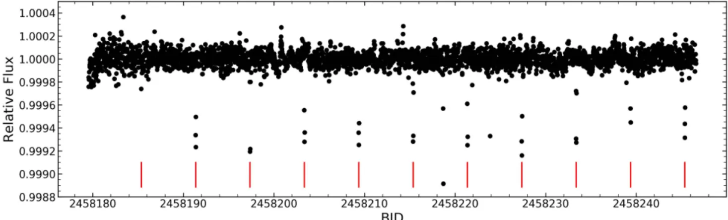
2.1. Photometry Extraction and Transit Detection The photometric extraction and transit detection methods used to identify Wolf503b are the same as those applied by our team to all light curves in C17 and are described in our corresponding C17 summary paper, Crossfield et al. (2018). As K2 operates using only two of Keplerʼs four initial reaction wheels, the telescope drifts along its roll axis by a few pixels every several days, and thrusterfirings are used to maintain the telescope’s pointing. The change in flux resulting from this drift is removed by fitting the flux as a function of position along the drift path, which is highly similar between thruster firings. However, the data acquired during these thruster burns are not reliable and are masked out, as in thefirst transit of the light curve for Wolf503, shown in Figure2.

With the extracted light curve, we detected a candidate at P=6.0 days with S/N=38 having 11 transits throughout the time of observation. The candidate was marked as a particularly intriguing KOI for its favorable host star following the manual vetting procedure of the C17 candidates.

2.2. Previous Work on Wolf503

Wolf503 (BD-05 3763, MCC 147, LHS 2799, G 64–24, HIP 67285, TYC 4973-1501-1, 2MASS J13472346-0608121) has been a sparsely studied nearby cool star since its discovery a century ago as a high proper motion star by Wolf(1919). The star subsequently appeared in several high proper motion catalogs over the past century, as Ci 20 806 in Porter et al. (1930), as G 64–24 in Giclas et al. (1961), and with Wilhelm Luyten designating the star no fewer than six times in his proper motion catalogs.15

The star was classified in numerous spectral survey as a K5V by Upgren et al.(1972, identified as UPG 336), and Bidelman (1985) published Kuiper’s posthumous classification for the star as K4 from his 1937 to 1944 survey. Pickles & Depagne (2010) found that the best-fit template for the BT VT J HKS

photometry was that for a K4V star.

2.2.1. Distance, Kinematics, and Stellar Population

Recently, Gaia DR2 provided an ultra-precise trigonometric parallax (ϖ=22.430 ± 0.048 mas; corresponding to d= 44.583± 0.096 pc), as well as precise proper motion and radial velocity measurements, which are listed in Table1. Gaia itself measured a radial velocity of −46.64±0.50 km s−1 (2 observations), and independently, Sperauskas et al. (2016) reported a radial velocity of −47.4±0.7 km s−1 based on 2 CORAVEL measurements over 98 days. Combining the Gaia DR2 position, proper motion, and parallax, and the mean Gaia DR2 ground-based radial velocity(from HARPS), we estimate

Figure 1.Observed planet radius distribution adapted from Fulton & Petigura (2018). There is a signiﬁcant decrease in the planet population from 1.5 to

2.0 R⊕. The 1σ radius limits for Wolf503b are overplotted in red and lie

directly adjacent to the radius gap, potentially indicating the planet is in the process of photoevaporation.

15

Entry#402 in Luyten (1923) (stars with motions exceeding 0 5 yr−1), as

LPM 492 in Luyten(1941), LFT 1037 in Luyten (1955), LHS 2799 in Luyten

(1979), and as NLTT 35228 and LTT 5351 in Luyten (1980).

(4)

a barycentric space velocity of U, V, W=−25.21, −116.86, −88.44 (±0.18, 0.21, 0.13) km s−1 _{(total velocity 148.71 ±}

0.18 km s−1), where U is toward the Galactic center, V is in the direction of Galactic rotation, and W is toward the north Galactic pole (Perryman et al. 1997). Using the velocity moments and local stellar population densities from Bensby et al.(2003), this UVW velocity is consistent with the following membership probabilities: <10−5%, 81%, 19%, for the thin disk, thick disk, and halo, respectively, highly indicative of kinematic membership to the thick disk population.

Mikolaitis et al. (2017) analyzed high-resolution, high-S/N HARPS spectra and found the star to be fairly metal-poor ([Fe/H] ; −0.37 based on two pairs of [FeI/H] and [FeII/H] abundances). Its combination of low metallicity, supersolar

[MgI/Fe] (∼0.28) and [ZnI/Fe] (0.19), and subsolar [MnI/Fe] (∼−0.16), led Mikolaitis et al. (2017) to chemically classify the chemical abundance data for Wolf503 as being consistent with membership in the thick disk. The thick disk shows a metallicity–age gradient (e.g., Bensby et al. 2004), and given Wolf503ʼs combination of [Fe/H] and [Mg/Fe] compared to age-dated thick disk members (Haywood et al. 2013), it is likely in the age range ∼9–13 Gyr. Hence, we adopt an age of 11±2 Gyr for Wolf503.

2.3. Spectroscopy and Stellar Parameters

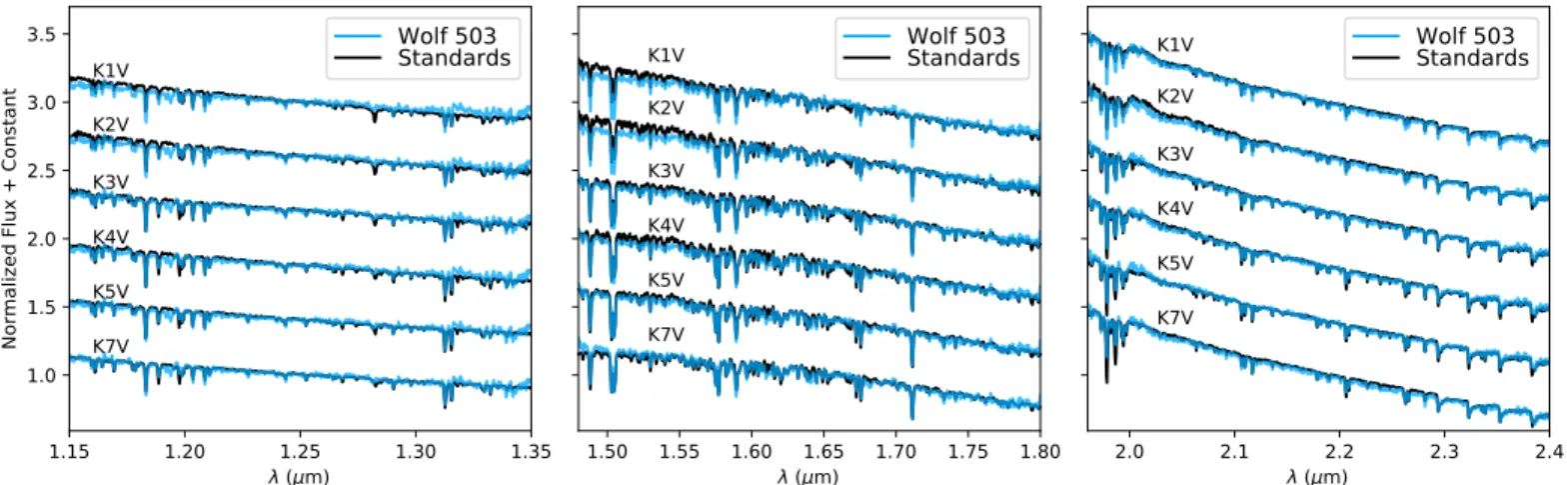
We obtained an R≈2000 infrared spectrum of Wolf503 covering the spectral range between 0.7 and 2.55μm at the NASA Infrared Telescope Facility (IRTF). We use the SpeX spectrograph in SXD mode with the 0 3×15″ slit. The spectrum was taken on UT 2018 June 03, on a partly cloudy night with an average seeing of 0 6. Reduction of the spectrum was performed with the SpeXTool (Cushing et al.2005) and xtellcor(Vacca et al. 2003) software packages as in Dressing et al.(2017). The sky subtraction was performed using a nearby A star, HD 122749, observed immediately after Wolf503b. The ﬁnal JHK band IRTF spectra of Wolf503 are shown in Figure 3 and compared to those of spectral standards. The best visual match indicates a spectral type of K3.5V±0.5, suggesting an effective temperature of approximately 4750±100 K from the SpeX spectrum.

During the vetting of candidates from C17 of K2 described in Crossfield et al. (2018), a spectrum was also obtained from the Tillinghast Reflector Echelle Spectrograph (TRES; Fűrész 2008) mounted on the 1.5 m Tillinghast Reflector at Fred Lawrence Whipple Observatory on Mount Hopkins on UT 2018 May 23. TRES is a fiber-fed, cross-dispersed echelle spectrograph with a resolving power of R∼44,000, a wavelength coverage of 3850–9100 Å, and radial velocity stability of 10–15m s-1_{. The spectrum was reduced and}

optimally extracted, and wavelength-calibrated according to the procedure described in Buchhave et al. (2010), and we derived stellar atmospheric parameters using the Stellar Parameter Classiﬁcation code (SPC; Buchhave et al. 2012). Weﬁnd Teff=4640±50 K, logg=4.68±0.10,[Fe H]=

-0.470.08, and vsini=0.8±0.5. We note that SPC

determines the stellar parameters using synthetic spectra with a ﬁxed macroturbulence of 1_{km s}-1_{, which may bias}



vsini measurements of slow rotators like this one. Regardless, Wolf

Table 1 Stellar Parameters

Parameter Value Source

Identifying Information α R.A. (hh:mm:ss) J2000 13:47:23.4439 δ Decl. (dd:mm:ss) J2000 −06:08:12.731 EPIC ID 212779563 Photometric Properties B(mag) 11.30±0.01 (Mermilliod1987) V(mag) 10.28±0.01 (Mermilliod1987) G(mag) 9.808±0.001 Gaia DR1 J(mag) 8.324±0.019 2MASS H(mag) 7.774±0.051 2MASS K(mag) 7.617±0.023 2MASS

Spectroscopic and Derived Properties

μα(mas yr−1) −343.833±0.073 Gaia DR2

μδ(mas yr−1) −573.134±0.073 Gaia DR2 Barycentric rv(km s−1) −46.826±0.015 Gaia DR2 Distance(pc) 44.583±0.096 Gaia DR2 Age(Gyr) 11±2 This Paper Spectral Type K3.5V±0.5 This Paper [Fe/H] −0.47±0.08 This Paper log g 4.62-+0.010.02 This Paper

Teff (K) 4716±60 This Paper M* (Me) 0.688-+0.0160.023 This Paper R* (Re) 0.690-+0.0240.025 This Paper L* (Le) 0.227-+0.0100.009 This Paper

Figure 2.Extracted light curve for Wolf503 (EPIC 212779563). Transit times according to our fit are indicated with a red line. The first observed transit is not easily visible in this plot because the transit coincided with a thruster burn during which two data points wereflagged and removed (see Figure6).

(5)

503 has a low projected rotational velocity, as is expected for an old K dwarf, which bolsters its status as a good candidate for precise radial velocity observations. We derive a barycentric radial velocity of −46.629±0.075km s-1_.

We conclude that the SpeX spectrum and the TRES spectrum result in consistent estimates of the stellar temper-ature. These values are also consistent with the value from the PASTEL catalog of 4759 K(Soubiran et al. 2010), as well as Wolf503ʼs colors (B − V = 1.02, V − K = 2.66), leading us to adopt the K3.5V±0.5 subtype.

Finally, we adopt Teff=4716±60 K, the average and scatter

of the three spectroscopic values, as ourﬁnal value for the stellar temperature. We then calculate the stellar parameters using Isoclassify(Huber et al.2017). Isoclassify uses measured stellar parameters in comparison to a sample of 2200 Kepler stars with combined Gaia and asteroseismic data in order to determine stellar parameters such as mass and radius with reliable uncertainty based on MIST models. We adopt the logg and [Fe H from the TRES spectrum, as well as the K magnitude,] which is least affected by extinction. We determine the best stellar radius estimate using the direct method in Isoclassify (Huber et al.2017), which uses bolometric corrections and direct physical relations to derive stellar properties, but does not return a mass. We obtain the stellar mass using the grid mode, which places the star on stellar evolutionary tracks to determine its properties. The two modes returned consistent stellar radii. The resulting stellar parameters are listed in Table1.

2.4. Target Validation

By far the most pernicious false positives detected in K2 data are eclipsing binaries, which may closely resemble exoplanet transits at grazing incidence, or when the binary system is found in the background of a brighter star (Abdul-Masih et al. 2016). We used archival and adaptive optics images to investigate the possibility of a false positive detection due to a companion star or background sources, andﬁnd no source in the vicinity of Wolf503 that could have contaminated our detection.

2.4.1. Adaptive Optics

Wolf503 was observed on the night of UT 2018 June 01 UT at Palomar Observatory with the 200″ Hale Telescope using the near-infrared adaptive optics(AO) system P3K and the infrared

camera PHARO (Hayward et al. 2001). PHARO has a pixel scale of 0 025 per pixel with a full field of view of approximately 25″. The data were obtained with a narrowband Br-γ filter (lo=2.18;D =l 0.03mm). The narrowness of the filter enables integration on the primary target without saturation, and the central wavelength of thefilter is sufficiently close to the central wavelength of the 2MASS Kshort filter

(λo= 2.15; Δλ = 0.31), enabling the deblending of the

2MASS magnitude of the primary star based on the observed magnitude difference of any detected companions.

The AO data were obtained in a five-point quincunx dither pattern with each dither position separated by 4″. Each dither position is observed three times, each offset from the previous image by 0 5 for a total of 15 frames; the integration time per frame was 4.428 s for a total of 66 s on-source integration time. We use the dithered images to remove sky background and dark current, and then align,flat-field, and stack the individual images. Thefinal PHARO AO data have a FWHM of 0 099. The sensitivities of the final combined AO image were determined by injecting simulated sources azimuthally around Wolf503 every 45◦ at separations of integer multiples of the

Figure 3.Final, calibrated SpeX spectra for Wolf503, shown compared to spectral standards. We ﬁnd that the best visual match for Wolf503 indicates a K3.5V±0.5 spectral type, consistent with previous classiﬁcations (see Section2.2).

Figure 4.Contrast sensitivity and inset image of Wolf503 in Br-γ as observed with the Palomar Observatory Hale Telescope adaptive optics system. The 5σ contrast limit is plotted against angular separation in arcseconds(ﬁlled circles). The shaded region represents the dispersion in the sensitivity caused by the azimuthal structure in the image(inset).

(6)

FWHM of the central source. The brightness of each injected source was scaled until standard aperture photometry detected it with 5σ signiﬁcance. The resulting brightness of the injected sources relative to Wolf503 set the contrast limits at that injection location. The average 5σ limits and associated rms dispersion caused by azimuthal asymmetries from residual speckles as a function of distance from the primary target are shown in Figure4.

The AO imaging revealed no additional stars within 0 099. For a system at a distance of 44.58pc, this limits the separation of a possible binary to less than 4.4 au.

2.4.2. Archival Images

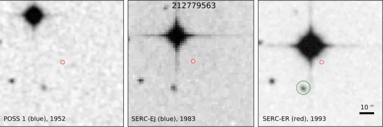
Even in the absence of a nearby contaminant, adaptive optics cannot eliminate the possibility of a background source directly behind the target, which could be responsible for the signal itself, or could otherwise decrease the apparent transit depth. To address this, we exploit archival imaging from the Palomar Observatory Sky Survey I, and the SERC-EJ and SERC-ER surveys taken on the UK Schmidt telescope. Figure5shows the present-day location of Wolf503 in each of the 3 surveys. The blue plate from POSS I (taken 1952 May 23) and the red SERC-ER survey image (taken on 1993 March 29 with the UK Schmidt Telescope) have a 1″ pixel scale, and the blue SERC-EJ image(taken 1983 May 7) has a 0 59 pixel scale.

The high proper motion of Wolf 503 reveals clearly that there is no background source at the star’s 2018 location. The object detected nearest to Wolf503ʼs present-day location is the galaxy LCRS B134447.1-055347, which is located≈25″1 from the target, placing it outside the aperture used in our extraction. Moreover, the galaxy has a Gaia magnitude of 19.6: being both 10 mag fainter and outside the aperture, we ﬁnd no background sources that may inﬂuence our photometry, indicating that any possible stellar contaminant must be bound within the limit of 4.4 au given by our adaptive optics.

As discussed in Section 2.5, the light curve is consistent either with a transiting planet or a highly speciﬁc multiple star system, therefore weﬁnd the likelihood of a false positive due to a bound eclipsing binary companion to be extremely low.

One scenario that remains plausible is the case of a bound companion orbiting within 4.4 au that does not transit Wolf 503, but contributes to the total ﬂux and dilutes the planet’s transit depth. According to the distribution of binary star systems found in Raghavan et al. (2010), fewer than 12% of stars belong to such close systems. Additionally, Kraus et al. (2016) found that binary systems with separations smaller than 50 au are not likely to host planets, and that planets in binary systems orbiting closer than 5 au are extremely rare, suggesting that this scenario is also not likely.

Such a companion would also induce a signiﬁcant radial velocity, of which there is no indication throughout measure-ments from Gaia, CORAVEL, and our team. Each of these measurements is consistent within 2σ and differs by less than 0.8km s-1_{. Even a 0.1}_M

ecompanion orbiting at 4.4 au would

induce a radial velocity of 1.6km s-1_{, and according to the}

modeled mass–luminosity relations in Spada et al. (2013), such a star would be roughly 4 mag dimmer in the K band and 9 mag dimmer in V, and would not signiﬁcantly affect the transit depth. The possibility of such a companion could conclusively be eliminated with high-resolution spectroscopy.

2.5. Light-curve Fitting

Wefit the light curve of Wolf503 using ExoFIT, a modular light-curve analysis tool developed for the joint analysis of data from Kepler, Spitzer, and HST. ExoFIT jointly or individually fits transits and explores the parameter space using the Affine Invariant Markov Chain Monte Carlo (AI-MCMC) Ensemble sampler available through the emcee package in Python. Details can be found in Benneke et al.(2017).

We performed individual transitfits in addition to fitting the transits simultaneously. For all fits, we initialize the MCMC chains with uniform priors using the best-fit values from the initial detection pipeline (see Section 2.1), and fit the transit start time T0, duration T14, depth Rp/R*, impact parameter b,

limb-darkening coefficient, and linear background for each transit and scatter term. For the jointfit, we also fit the period P. In each fit, we assign 6 walkers for each parameter and find good convergence after 3000 steps, taking the initial 60% as burn-in.

Figure 5.Archival images from the blue plate of the POSS I sky survey(with a limiting magnitude of 21.0, taken 1952 May 23), from the blue SERC-EJ survey taken at the UK Schmidt Telescope(with a limiting magnitude of 23.0 taken 1983 May 7), and from the red SERC-ER survey also taken at UKST (with a limiting magnitude of 22.0, taken on 1993 May 27). Wolf503ʼs signiﬁcant high proper motion is clear in the sequence of images, and there are no background sources detected at its 2018 location marked in red(R.A. = 13h47h23 031, decl.= −06d08m23 047, calculated using the Gaia DR2 proper motion measurements). The nearest source is the faint galaxy LCRS B134447.1–055347, circled in green in the right panel, which is both 10 mag fainter than Wolf503 and found outside our extraction aperture.

(7)

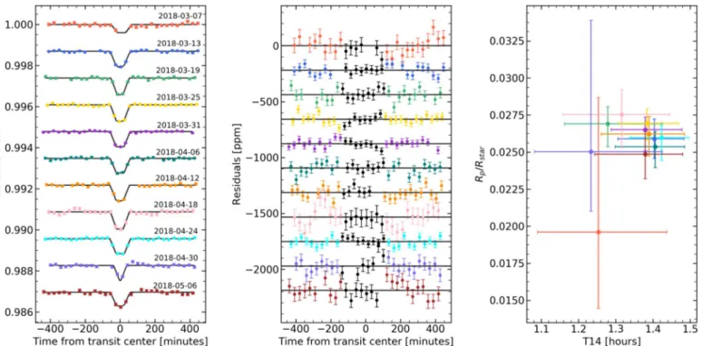
The transits werefirst fit individually, and the resulting fits are shown in Figure 6. Of the 11 transits observed, all are consistent in Rp/R*and T14. We obtain our best-fitting planet

parameters from a joint ﬁt of the 11 transits using the initialization as previously described. The parameters resulting from thisﬁt are summarized in Table2, where the errors in Rp

and a are dominated by the stellar parameters. The best-ﬁt light curve is shown in Figure7, where the combined residuals are well-behaved.

The bestfit is distinctly flat-bottomed, inconsistent with the V-shaped light curves characteristic of eclipsing binaries, unless Wolf 503 belongs to a trinary system with two smaller stars orbiting on a 12 day period, within 4.4 au, aligned to be completely eclipsing. In addition to being far more contrived than a single transiting planet, the depth and duration of the transits in Figure 6 are highly regular, and do not show the even–odd variation that would be expected of such an eclipsing binary. As discussed in Section 2.4, such a companion would also induce a significant radial velocity, which has not been detected and would be easily revealed using high-resolution spectroscopy.

3. Discussion

From our combined imaging, photometric, and spectral analyses, we establish Wolf503b as a 2.03_-+0.070.08RÅ planet

orbiting its K3.5V±0.5 dwarf host star with a period of 6.0012 days. Wolf503b is truly distinguished, as its size places it directly at the edge of the radius gap near 1.5–2.0 R_⊕, while its bright host star (H = 7.77 mag, V = 10.28 mag) makes it one of the best targets for radial velocity follow-up and transit spectroscopy at its size(Figure8).

Radial velocity measurements of Wolf503b present an excellent opportunity to probe the bulk density of a planet just outside the radius gap. The amplitude of the expected RV

signal depends strongly on the planet composition and amount of gas accreted. As Wolf503b is similar in size to 55 Cnc e, though at a lower temperature, we investigate its composition using the mass–radius relationships for rocky compositions found in Valencia et al.(2010) and Gillon et al. (2012). For the gas-poor scenario, the minimum mass required for a rocky composition (with no iron), is roughly 10 M_⊕, with an Earth-like composition corresponding to 14 M_⊕. These masses would result in RV amplitudes of roughly 4.5 and 6.3 m s−1. For a volatile planet with a 0.01% H/He envelope, we would expect a mass of roughly 8 M_⊕, whereas a 20% water envelope would suggest 6 M_⊕, and the empirical mass–radius relation by Weiss et al.(2013) would suggest 5.3 M_⊕, giving RV amplitudes of 3.6, 2.7, and 2.4 m s−1. These amplitudes are detectable with existing precision radial velocity spectrographs, particularly for a bright target such as Wolf503. As the gas-rich scenario produces much smaller RV amplitudes, these measurements will provide critical constraints on the bulk composition of the planet.

Figure 6.Individual K2 transitfits of Wolf503b. The left panel shows each individual transit with its corresponding best-fit model. The residuals are shown in the center panel, with the residuals in the range T0±T14marked in black. The right plot shows the best guess and 1σ, or 68% confidence limits on the Rp/R* and T14

parameters, which are consistent for all transits, further supporting the argument that the signal best matches that of a transiting planet. Uncertainties on theﬁrst and tenth transits(red and violet) are higher due to masked data points coinciding with a thruster burn near the time of the transit.

Table 2 Planet Parameters

Parameter Units Value

T0 BJDTBD–2457000 1185.36087-+0.000380.00053 P day 6.00118-+0.000110.00008 Rp/R* % 2.694-+0.0260.026 T14 hr 1.321-+0.0390.051 b L 0.387-+0.0610.067 Rp R⊕ 2.030-+0.0730.076 a au 0.0571±0.0020 S S⊕ 69.6±3 Teq, A= 0 K 805±9

(8)

Wolf503b is also an ideal target for detailed characterization with HST and JWST. The signal to noise for future HST transit spectroscopy was estimated in comparison to other conﬁrmed planets near the radius gap, assuming a volatile-rich H/He envelope for each planet. Using the same estimated planet mass of 5.3M_⊕, Wolf 503b is expected to be the second best candidate, behind only 55 Cnc e, for studying a planet in the 1.8–2.1 R_⊕range, where planets may be transitioning into the radius gap through photoevaporation. The planet is also approximately 1000 K cooler than 55 Cnc e, making it much more likely to have a signiﬁcant H2fraction in its atmosphere,

but may also be in the process of photoevaporation. With J=8.32 mag, it is just below the saturation levels of J>7 mag and J>6 mag on the NIRISS and NIRSpec grisms. If Wolf503b indeed harbors a thick atmosphere, it is one of the best known targets to date for transmission spectroscopy at its size. Figure 9 shows two simulated transit spectra for Wolf503b, the blue corresponding to a hydrogen-rich, Neptune-like atmosphere, and the orange corresponding to an atmosphere rich in water. Simulated NIRISS and NIRSpec data

for the Neptune-like atmosphere is overplotted, demonstrating the high-conﬁdence with which we will be able to constrain the structure and abundances of atmospheric molecules on Wolf503b.

Both radial velocity measurements and atmospheric char-acterization with HST would be valuable short-term follow-up to this work. Wolf 503b is among only a handful of planets in its size range for which this follow-up can be done efﬁciently today. As such, we expect Wolf 503b to play a critical role in providing near-term insights into the distribution of core masses, the envelope fraction, and the role of photoevaporation for planets near the Fulton gap. It can also serve as an archetype for this class of small planets orbiting nearby stars in preparation for future characterization of similarly bright TESS systems.

Figure 7.Final light-curvefit from ExoFIT for the combined 11 transits. In the top panel, the bestfit is shown in black with the detrended light curves for each transit. Accounting for the 30 minute cadence of the K2 data gives the bestfit its trapezoidal shape. The residuals are plotted in the middle panel, and are binned in the histogram in the bottom pane; by the number ofσ from the best fit, where they follow a standard normal distribution of the same area.

Figure 8.Planet radius and stellar host magnitude of Wolf503b (larger circle) in comparison to all planets at the NASA Exoplanet Archive(colored points). The color of the points indicates the stellar temperature. Planets in a similar size range orbiting bright stars are labeled. Wolf503 is among the brightest systems with a planet near 2 R⊕detected to date.

Figure 9. Model transit spectra and simulated JWST observations for Wolf503b. Observations of a single transit with JWST/NIRISS (green) or JWST/NIRSpec (red) could readily detect molecular absorption for hydrogen-dominated, cloud-free atmospheres(blue). The planetary mass assumed in the models is 5.3 M⊕. Models are computed as described in Benneke & Seager

(2012) and Benneke (2015). Simulated observational uncertainties are from

(9)

We acknowledge support from NASA through K2GO grant 80NSSC18K0308 and from NSF through grant AST-1824644. This paper includes data collected by the Kepler mission. Funding for the Kepler mission is provided by the NASA Science Mission directorate. Some of the data presented in this paper were obtained from the Mikulski Archive for Space Telescopes (MAST). STScI is operated by the Association of Universities for Research in Astronomy, Inc., under NASA contract NAS526555. Support for MAST for nonHST data is provided by the NASA Ofﬁce of Space Science via grant NNX13AC07G and by other grants and contracts. This research has made use of the Exoplanet Follow-up Observing Program (ExoFOP), which is operated by the California Institute of Technology, under contract with the National Aeronautics and Space Administration. Part of this research was carried out at the Jet Propulsion Laboratory, California Institute of Technology, under a contract with the National Aeronautics and Space Administration. E.E.M. and T.J.D. acknowledge support from the JPL Exoplanet Science Initiative. E.E.M. acknowledges support from the NASA NExSS program.

Facilities: Kepler, K2, Palomar, IRTF, FLWO:1.5m(TRES). ORCID iDs

Trevor J. David https://orcid.org/0000-0001-6534-6246 Courtney D. Dressing https: //orcid.org/0000-0001-8189-0233

Joshua E. Schlieder https://orcid.org/0000-0001-5347-7062 Erik A. Petigura https://orcid.org/0000-0003-0967-2893 Eric E. Mamajek https://orcid.org/0000-0003-2008-1488 Jessie L. Christiansen https: //orcid.org/0000-0002-8035-4778

Sam N. Quinn https://orcid.org/0000-0002-8964-8377 Benjamin J. Fulton https://orcid.org/0000-0003-3504-5316 Andrew W. Howard https:

//orcid.org/0000-0001-8638-0320

Evan Sinukoff https://orcid.org/0000-0002-5658-0601 David W. Latham https://orcid.org/0000-0001-9911-7388 Liang Yu https://orcid.org/0000-0003-1667-5427

Avi Shporer https://orcid.org/0000-0002-1836-3120 Molly R. Kosiarek https://orcid.org/0000-0002-6115-4359

References

Abdul-Masih, M., Prša, A., Conroy, K., et al. 2016,AJ,151, 101

Batalha, N. E., Mandell, A., Pontoppidan, K., et al. 2017,PASP,129, 064501

Batalha, N. M., Rowe, J. F., Bryson, S. T., et al. 2013,ApJS,204, 24

Benneke, B. 2015, arXiv:1504.07655

Benneke, B., & Seager, S. 2012,ApJ,753, 100

Benneke, B., Werner, M., Petigura, E., et al. 2017,ApJ,834, 187

Bensby, T., Feltzing, S., & Lundström, I. 2003,A&A,410, 527

Bensby, T., Feltzing, S., & Lundström, I. 2004,A&A,421, 969

Bidelman, W. P. 1985,ApJS,59, 197

Buchhave, L. A., Bakos, G. Á, Hartman, J. D., et al. 2010,ApJ,720, 1118

Buchhave, L. A., Latham, D. W., Johansen, A., et al. 2012,Natur,486, 375

Crossﬁeld, I. J. M., Guerrero, N., David, T., et al. 2018, arXiv:1806.03127

Cushing, M. C., Rayner, J. T., & Vacca, W. D. 2005,ApJ,623, 1115

Dressing, C. D., Vanderburg, A., Schlieder, J. E., et al. 2017,AJ,154, 207

Dumusque, X., Bonomo, A. S., Haywood, R. D., et al. 2014,ApJ,789, 154

Fressin, F., Torres, G., Charbonneau, D., et al. 2013,ApJ,766, 81

Fulton, B. J., & Petigura, E. A. 2018, arXiv:1805.01453

Fulton, B. J., Petigura, E. A., Howard, A. W., et al. 2017,AJ,154, 109

Fűrész, G. 2008, PhD thesis, Univ. Szeged

Giclas, H. L., Burnham, R., & Thomas, N. G. 1961, LowOB,5, 61

Gillon, M., Demory, B.-O., Benneke, B., et al. 2012,A&A,539, A28

Hayward, T. L., Brandl, B., Pirger, B., et al. 2001,PASP,113, 105

Haywood, M., Di Matteo, P., Lehnert, M. D., Katz, D., & Gómez, A. 2013,

A&A,560, A109

Howard, A. W. 2013,Sci,340, 572

Huber, D., Zinn, J., Bojsen-Hansen, M., et al. 2017,ApJ,844, 102

Ida, S., & Lin, D. N. C. 2004,ApJ,604, 388

Jin, S., & Mordasini, C. 2018,ApJ,853, 163

Kraus, A. L., Ireland, M. J., Huber, D., Mann, A. W., & Dupuy, T. J. 2016,AJ,

152, 8

Lee, E. J., Chiang, E., & Ormel, C. W. 2014,ApJ,797, 95

Lopez, E. D., & Rice, K. 2016, arXiv:1610.09390

Luyten, W. J. 1923,LicOB,11, 1

Luyten, W. J. 1941, POMin,3, 1

Luyten, W. J. 1955, Luyten’s Five Tenths,1054, 0

Luyten, W. J. 1979, LHS Catalogue. A Catalogue of Stars with Proper Motions Exceeding 0 5 Annually(Minneapolis, MN: Univ. Minnesota Press) Luyten, W. J. 1980, NLTT Catalogue, Volume_III. 0__to−30_ (Minneapolis,

MN: Univ. Minnesota Press) Mermilliod, J. C. 1987, BICDS,32, 37

Mikolaitis,Š, de Laverny, P., Recio-Blanco, A., et al. 2017,A&A,600, A22

Mordasini, C., Alibert, Y., & Benz, W. 2009,A&A,501, 1139

Mullally, F., Coughlin, J. L., Thompson, S. E., et al. 2015,ApJS,217, 31

Owen, J. E., & Wu, Y. 2013,ApJ,775, 105

Perryman, M. A. C., Lindegren, L., Kovalevsky, J., et al. 1997, A&A,323, L49

Pickles, A., & Depagne, É. 2010,PASP,122, 1437

Pollack, J. B., Hubickyj, O., Bodenheimer, P., et al. 1996,Icar,124, 62

Porter, J. G., Yowell, E. J., & Smith, E. S. 1930, PCinO,20, 1

Raghavan, D., McAlister, H. A., Henry, T. J., et al. 2010,ApJS,190, 1

Rogers, L. A. 2015,ApJ,801, 41

Soubiran, C., Campion, J.-F. L., Strobel, G. C. d., & Caillo, A. 2010,A&A,