HAL Id: hal-03001722
https://hal.archives-ouvertes.fr/hal-03001722
Submitted on 12 Nov 2020
HAL is a multi-disciplinary open access
archive for the deposit and dissemination of
sci-entific research documents, whether they are
pub-lished or not. The documents may come from
teaching and research institutions in France or
abroad, or from public or private research centers.
L’archive ouverte pluridisciplinaire HAL, est
destinée au dépôt et à la diffusion de documents
scientifiques de niveau recherche, publiés ou non,
émanant des établissements d’enseignement et de
recherche français ou étrangers, des laboratoires
publics ou privés.
RAS-NAAD: 40-yr High-Resolution North Atlantic
Atmospheric Hindcast for Multipurpose Applications
(New Dataset for the Regional Mesoscale Studies in the
Atmosphere and the Ocean)
Alexander Gavrikov, Sergey Gulev, Margarita Markina, Natalia Tilinina,
Polina Verezemskaya, Bernard Barnier, Ambroise Dufour, Olga Zolina, Yulia
Zyulyaeva, Mikhail Krinitskiy, et al.
To cite this version:
Alexander Gavrikov, Sergey Gulev, Margarita Markina, Natalia Tilinina, Polina Verezemskaya, et al..
RAS-NAAD: 40-yr High-Resolution North Atlantic Atmospheric Hindcast for Multipurpose
Applica-tions (New Dataset for the Regional Mesoscale Studies in the Atmosphere and the Ocean). Journal
of Applied Meteorology and Climatology, American Meteorological Society, 2020, 59 (5), pp.793-817.
�10.1175/JAMC-D-19-0190.1�. �hal-03001722�
RAS-NAAD: 40-yr High-Resolution North Atlantic Atmospheric Hindcast for
Multipurpose Applications (New Dataset for the Regional Mesoscale Studies in
the Atmosphere and the Ocean)
ALEXANDERGAVRIKOV,aSERGEYK. GULEV,a,bMARGARITAMARKINA,a,bNATALIATILININA,a POLINAVEREZEMSKAYA,aBERNARDBARNIER,a,cAMBROISEDUFOUR,a,cOLGAZOLINA,a,c
YULIAZYULYAEVA,aMIKHAILKRINITSKIY,aIVANOKHLOPKOV,bANDALEXEYSOKOVa
aP.P. Shirshov Institute of Oceanology, Russian Academy of Sciences, Moscow, Russia bMoscow State University, Moscow, Russia
cInstitut des Géosciences de l’Environnement, Grenoble, France
(Manuscript received 2 August 2019, in final form 3 March 2020)
ABSTRACT
We present in this paper the results of the Russian Academy of Sciences North Atlantic Atmospheric Downscaling (RAS-NAAD) project, which provides a 40-yr 3D hindcast of the North Atlantic (108–808N) atmosphere at 14-km spatial resolution with 50 levels in the vertical direction (up to 50 hPa), performed with a regional setting of the WRF-ARW 3.8.1 model for the period 1979–2018 and forced by ERA-Interim as a lateral boundary condition. The dataset provides a variety of surface and free-atmosphere parameters at sigma model levels and meets many demands of meteorologists, climate scientists, and oceanographers working in both research and operational domains. Three-dimensional model output at 3-hourly time resolution is freely available to the users. Our evaluation demonstrates a realistic representation of most characteristics in both datasets and also identifies biases mostly in the ice-covered regions. High-resolution and nonhydrostatic model settings in NAAD resolve mesoscale dynamics first of all in the subpolar lati-tudes. NAAD also provides a new view of the North Atlantic extratropical cyclone activity with a much larger number of cyclones as compared with most reanalyses. It also effectively captures highly localized mechanisms of atmospheric moisture transports. Applications of NAAD to ocean circulation and wave modeling are demonstrated.
1. Introduction
Subsynoptic and mesoscale atmospheric dynamics over the North Atlantic Ocean are of great interest for understanding the mechanisms of highly localized pre-cipitation, heat and moisture transports, and low-level baroclinicity in the atmosphere. Changes in the intensity and location of the North Atlantic storm tracks are critically important for the quantification of the impact of highly variable atmospheric processes onto air–sea fluxes and associated ocean signals and for understand-ing the responses of cyclone activity to those ocean signals (Minobe et al. 2008,2010;Woollings et al. 2012; Tilinina et al. 2018). Many works hint at the critical role
of mesoscale dynamics in air–sea interaction in the North Atlantic, first of all in forming cold-air outbreaks (Zolina and Gulev 2003;Bond and Cronin 2008;Papritz et al. 2015;Kim et al. 2016) over the Gulf Stream, the Labrador Sea, and the Greenland–Iceland–Norwegian (GIN) Seas and in generating polar lows characterized by small scales and extreme surface fluxes in the sub-polar regions (Kolstad 2011; Condron and Renfrew 2013;Stoll et al. 2018, among others). Extremely high turbulent heat and momentum surface fluxes associated with these phenomena are highly localized in space and in time and require high temporal and spatial resolution for their adequate representation in models (Gulev and Belyaev 2012;Vihma et al. 2014).
Many lower-troposphere responses to the ocean sig-nals are also associated with mesoscale processes, includ-ing the low-level baroclinicity over the western boundary currents (Nakamura et al. 2012; Ogawa et al. 2012; Small et al. 2014;Ma et al. 2017;DuVivier et al. 2016;
Denotes content that is immediately available upon publica-tion as open access.
Corresponding author: Sergey K. Gulev, gul@sail.msk.ru
DOI: 10.1175/JAMC-D-19-0190.1
Ó 2020 American Meteorological Society. For information regarding reuse of this content and general copyright information, consult theAMS Copyright Policy(www.ametsoc.org/PUBSReuseLicenses).
Parfitt et al. 2016, 2017) and anomalous convective precipitation in warm seasons (Minobe et al. 2008; Hand et al. 2014). High-resolution regional model ex-periments demonstrated the responses of the lower atmosphere to the ocean signals at length scales of less than 30–50 km, suggesting ocean–atmosphere coupling at mesoscales and submesoscales (Small et al. 2008, 2014,2019;Ma et al. 2017;Parfitt et al. 2016;Bishop et al. 2017). Subsynoptic and mesoscale processes are also crucial for better understanding the mechanisms of atmospheric moisture transports, first of all in the at-mospheric rivers (ARs;Lavers et al. 2011;Lavers and Villarini 2015; Gimeno et al. 2014) providing strong ocean-to-continent moisture intrusions associated with abundant precipitation. All of these phenomena can-not always be adequately captured by global rean-alyses, such as ERA-Interim, JRA-55, MERRA-2, and ERA5 (Dee et al. 2011;Kobayashi et al. 2015; Gelaro et al. 2017; Copernicus Climate Change Service 2017; for definitions of acronyms, seehttps:// www.ametsoc.org/PubsAcronymList), partly because of their relatively coarse resolution but also because of the use of hydrostatic model configurations. Remarkably, the Arctic System Reanalysis (ASR; Bromwich et al. 2016,2018) performed with the polar Weather Research and Forecasting (WRF) Model (Bromwich et al. 2009) demonstrated a considerable improvement of the representation of many phe-nomena in the Arctic atmosphere (Tilinina et al. 2014; Moore et al. 2015,2016;Smirnova and Golubkin 2017; Boisvert et al. 2018;Justino et al. 2019, among others).
Ongoing ocean modeling activities also require high-resolution forcing functions accounting for mesoscale atmo-spheric features. Existing datasets used for forcing model experiments such as Drakkar forcing set (DFS4/5), Coordinated Ocean-Ice Reference Experiments (CORE), and JRA-55-do are based on global reanalyses (Large and Yeager 2004,2009;Brodeau et al. 2010;Danabasoglu et al. 2014,2016;Tsujino et al. 2018) with a spatial resolution of approximately 50–100 km. At the same time, modern eddy-resolving ocean general circulation models use resolutions finer than 1/108, equivalent to a few kilo-meters at subpolar latitudes (Deshayes et al. 2013; Sérazin et al. 2015;Guo et al. 2014;Rudnick et al. 2015; Behrens et al. 2017), and up to 1/508–1/608 in some re-gional simulations (Chassignet and Xu 2017; Fresnay et al. 2018;Fallmann et al. 2019). These experiments are focused on essentially small-scale ocean features. The role of small-scale atmospheric processes, however, re-mains unclear when using relatively coarse-resolution forcing. Similarly, modern spectral wave models account for highly nonlinear wave generation and development processes strongly dependent on the submesoscale wind
structure (Ardhuin et al. 2012; Hanley et al. 2010; Semedo et al. 2011;Zieger et al. 2015;Markina et al. 2019). At the same time, in most cases these advanced configurations are forced with relatively coarse-resolution reanalysis winds.
In summary, there is a high demand from different communities for long-term high-resolution atmospheric hindcasts performed with high-resolution model con-figurations for the North Atlantic where mesoscale and submesoscale processes are of high relevance. Facing this challenge, the P.P. Shirshov Institute of Oceanology of the Russian Academy of Sciences (IORAS) in cooperation with the Institut des Géosciences de l’Environnement (IGE) developed a high-resolution (14 km) atmospheric downscaling experiment for the North Atlantic Ocean [North Atlantic Atmospheric Downscaling (NAAD)]. In NAAD, the nonhydrostatic WRF Model was forced at the lateral boundaries by the ERA-Interim reanalysis over the 40-yr period (1979– 2018). In the following, we describe the NAAD model configuration and production strategy in section 2 fol-lowed by a short description of NAAD products and data availability (section 3). Then we turn to the NAAD evaluation (section 4) and pilot applications (section 5). In the conclusivesection 6we discuss the NAAD added value and perspectives of further developments of the product.
2. NAAD model configuration and production strategy
In NAAD we used the nonhydrostatic WRF Model, version 3.8.1 (Skamarock et al. 2008;Powers et al. 2017). The domain covers the North Atlantic from 108 to 808N and from 908W to 58E (Fig. 1), with the center at 458N, 458W. The initial and lateral boundary conditions [in-cluding sea surface temperature (SST)] were provided by the ERA-Interim reanalysis (Dee et al. 2011) at 0.78 3 0.78 spatial resolution and 60 levels in the vertical direction. The spatial resolution in the basic NAAD high-resolution experiment (HiRes) was 14 km (5513 551 points) and 50 terrain-following, dry hydrostatic pressure levels, starting from around 10–12 m above the ocean surface to 50 hPa with;15 levels in the boundary layer (http://www.naad.ocean.ru). Besides the HiRes experiment, we also conducted a moderately low reso-lution experiment (LoRes) with the hydrostatic setting of the WRF Model at 77-km resolution (110 3 110 points) with 50 vertical levels (as in HiRes). The LoRes experiment (with resolution comparable to ERA-Interim) will be used to quantify the added value of the HiRes experiment, which cannot be di-rectly compared with ERA-Interim (constrained by 794 J O U R N A L O F A P P L I E D M E T E O R O L O G Y A N D C L I M A T O L O G Y VOLUME59
data assimilation and using a very different model configuration). All experiments were run for the 40-yr period from January 1979 to December 2018. Details of the model settings for the HiRes and LoRes ex-periments are presented inTable 1.
Most parameterizations were used in both HiRes and LoRes NAAD experiments. We used the Kain– Fritsch (KF) convective parameterization scheme (Kain 2004). The RRTMG longwave and shortwave
radiation schemes (Iacono et al. 2008) were used for terrestrial and solar radiation processes, which addi-tionally utilize effective cloud water, ice and snow radii from the single-moment 6-class (WSM6) scheme for microphysics (Hong and Lim 2006) in HiRes, and subgrid convective cloud information from KF for a more accurate estimation of atmospheric optical depth. The surface layer was parameterized by the MM5 scheme of (Skamarock et al. 2008) based upon similarity theory, accounting for a viscous sublayer and incorpo-rating the COARE 3.0 algorithm (Fairall et al. 2003) for calculating thermal and moisture roughness lengths (or exchange coefficients for heat and moisture) over the ocean surface. For the planetary boundary layer (PBL) we used the Yonsei University (YSU) nonlocal scheme (Hong et al. 2006) and the Noah land surface model (Chen and Dudhia 2001). An important issue is the number of vertical levels captured by the PBL. In NAAD (see the specification of vertical levels athttp:// www.naad.ocean.ru), 15 vertical levels are below 850 hPa. Computation of the PBL height (not shown) reveals the highest PBL exceeding 1000 m over the regions with active convection and the lowest PBL of less than 200 m in the polar regions. This implies that the number of vertical levels in PBL range from as few as 5–6 to as many as 15–16 over the NAAD domain. In this respect, for example, version 2 of ASR (ASRv2;Bromwich et al. 2018) with approximately 10–12 levels in the PBL (implied by 25 levels below
TABLE1. NAAD HiRes and LoRes experimental design (see text for details).
Attribute Setting
General
Model WRF-ARW 3.8.1
Name of expt LoRes HiRes
Dynamical core Hydrostatic Nonhydrostatic
Grid and time configuration
Horizontal grid type Arakawa C grid staggered
Horizontal resolution 77 km 14 km
Vertical coordinate type Terrain-following, dry hydrostatic pressure Vertical resolution, no. of levels 50
Time-stepping scheme Time-split integration using a third-order Runge–Kutta scheme
Time step (s) 240 30
Physical parameterizations
Microphysics scheme WSM5 (Hong et al. 2004) WSM6 (Hong and Lim 2006) Cumulus scheme Kain–Fritsch (Kain 2004)
PBL scheme YSU (Hong et al. 2006)
Surface-layer scheme MM5 (Skamarock et al. 2008) Radiative transfer (short- and longwave) RRTMG (Iacono et al. 2008) Land surface model Noah LSM (Chen and Dudhia 2001)
Boundary conditions
Initial and boundary conditions ERA-Interim (spectral nudging longer than 1100 km)
SST ERA-Interim
FIG. 1. NAAD computational domain and map-scale factor for the HiRes simulation.
850 hPa) is more effective in polar latitudes; however, ASRv2 is based on the local Mellor–Yamada–Janjic´ PBL scheme, which may not necessarily be effective over the whole North Atlantic region.
Since the Noah scheme updates deep soil temperature, the skin sea surface temperature is calculated using the Zeng and Beljaars (2005)formulation. The PBL scheme is responsible for vertical subgrid-scale fluxes due to eddy transports in the whole atmospheric column, and not only in the boundary layer. Horizontal eddy viscosity coeffi-cients are obtained in the WRF dynamic core indepen-dently using the Smagorinsky first-order closure approach. Parameterizations of microphysics were nevertheless different in HiRes and LoRes. Thus, the WSM6 scheme for microphysics (Hong and Lim 2006) was used in the NAAD-HiRes and WSM 5-class (WSM5; Hong et al. 2004). Additionally, employing entrain-ment information from KF was applied in the NAAD-LoRes case. For the long-term runs with WRF in both HiRes and LoRes experiments, the RRTMG scheme uses climatological ozone and aerosol data. The ozone data were adapted from the Community Atmospheric Model radiation scheme with latitudinal (2.828 step), height, and temporal (monthly) variation. The aerosol data were based on the Tegen et al. (1997)dataset with relatively coarse spatial (58 in longitude and 48 in latitude) and temporal (monthly) resolution.
The WRF settings used for NAAD HiRes, with some modifications, was applied in a number of applications. In the Polar WRF used in ASRv2 (Bromwich et al. 2018) the major difference was in the use of the Mellor–Yamada– Nakanishi–Niino (Nakanishi 2001; Nakanishi and Niino 2004,2006) 2.5-level PBL parameterization. However, the nonlocal YSU scheme used in NAAD is effective to resolve strong convective processes in the midlatitudes and tropical regions. This parameterization was used in a number of RCM simulations (Bukovsky and Karoly 2009;Otte et al. 2012;Gao et al. 2015;Tang et al. 2017).
At the ocean surface, we used ERA-Interim SST and sea ice, which was updated every 6 h during the simulation. ERA-Interim SST is combined from different sources (Dee et al. 2011).Kumar et al. (2013)demonstrated that in different reanalyses, the intraseasonal SST–precipitation relationship is dependent on the SST used. In this respect we understand that the relatively coarse (with respect to HiRes) resolution of ERA-Interim SST may have an effect on the atmospheric surface layer and PBL. Currently, several high-resolution SST datasets, while limited in time coverage, are available (Chelton and Wentz 2005;Chao et al. 2009;Ricchi et al. 2016). Nevertheless, for the 40-yr-long NAAD experiments we used ERA-Interim SST, which is considered to be homogeneous and adequate for multidecadal scales.
To reduce unrealistic atmospheric dynamics in the regional domain in both LoRes and HiRes experiments, we applied throughout the 40-yr period the procedure of spectral interior nudging (Jeuken et al. 1996; Miguez-Macho et al. 2004). The spectral nudging technique optimizes the adjustment of the large-scale dynamics inside the domain to that implied by the boundary conditions. The nudging procedure was applied to the zonal and meridional wind components, air tempera-ture, and the perturbation of the geopotential height. We did not nudge the moisture fields because their variability is not always represented adequately in the coarse-resolution ERA-Interim (Miguez-Macho et al. 2004;Otte et al. 2012). Configuration of nudging was set according to the sensitivity study of Markina et al. (2018), which implied the optimal wavelength cutoff being 1100 km, applied only above the PBL. For de-termining the optimal nudging strength, we performed sensitivity experiments with the nudging strength co-efficients increasing from 3 3 1025 to 3 3 1023s21. These experiments implied an optimal value of the nudging strength coefficient of 33 1024s21(equivalent to a damping scale of about 1 h). This value is also con-sistent with other studies (Miguez-Macho et al. 2004;Otte et al. 2012;Tang et al. 2017, among others). Note also that the ASRv2 (Bromwich et al. 2018) used spectral nudging with the strength 33 1023s21(i.e., an order of magnitude stronger relative to NAAD) for all levels in the outer do-main and above 100 hPa in the inner dodo-main. However, a direct comparison is unlikely to be possible here, as the ARSv2 assimilates a lot of observational data in the surface layer using the same technique (Newtonian relaxation, also called ‘‘observational nudging’’;Jeuken et al. 1996).
The dynamical solver of WRF uses a Cartesian grid. The difference between the geographical and the model hori-zontal distance (map-scale factor) should not deviate sig-nificantly from unity in order to match the CFL criterion. The NAAD grid is based on a cylindrical equidistant pro-jection (lat-lon in the namelist;http://www.naad.ocean.ru) with the rotated pole in order to locate the equator at the middle of the domain ( pole_lat5 45; pole_lon 5 180; stand_lon 5 245). For this projection, the maximum map-scale factor amounts to 1.2 in the northernmost and southernmost regions of the domain (Fig. 1). This allowed for keeping a constant third-order Runge– Kutta time step of 30 s in HiRes and 240 s in LoRes. In NAAD we used the USGS topography data with 10 min spatial resolution.
3. NAAD products and data availability
NAAD products (see http://www.naad.ocean.ru for the parameter identification and namelist) include 796 J O U R N A L O F A P P L I E D M E T E O R O L O G Y A N D C L I M A T O L O G Y VOLUME59
surface and upper-troposphere variables provided at the native NAAD grid for HiRes and LoRes products with resolutions of 14 and 77 km, respectively, for the period of 1979–2018. Since the NAAD core model (WRF-ARW) uses a staggered Arakawa C grid, all 3D fields are preinterpolated from the C grid on the mass points (unstaggered grid). No interpolation was applied for surface variables and fluxes, provided at the mass points. The entire archive of the NAAD data amounts to 150 terrabytes (TB) with individual annual files ranging from approximately 140 MB in LoRes to 3.3 GB in HiRes for surface variables on to 165 GB for HiRes 3D fields. The whole NAAD data output is organized as annual NetCDF files by variable and is available online (http://www.naad.ocean.ru) for download using FTP and Network Data Access Protocol (OPeNDAP) accesses. 4. NAAD evaluation
a. Surface
Surface-state variables and fluxes are particularly significant as they are used for forcing ocean models and
for the diagnostics of extreme events.Figures 2a and 2b show that surface air temperature diagnosed by NAAD HiRes is colder than in LoRes. The differences between LoRes and HiRes are smaller than 0.28C over most of the domain and increase to 0.48C in the western mid-latitude North Atlantic. Larger surface air temperatures in HiRes compared to LoRes, amounting to 18C, are observed over the ice-covered regions and occur pri-marily in the winter months. This regional bias can be explained by using a coarse-resolution sea ice mask from ERA-Interim in both HiRes and LoRes NAAD simu-lations. Compared to ERA-Interim (Fig. 2c), HiRes shows 0.28 to 0.48C lower surface air temperatures over most of the North Atlantic and considerably colder surface air temperatures in the ice-covered regions in the subpolar North Atlantic. A similar pattern of dif-ferences in surface air temperature is revealed for ASRv2 (Fig. 2d) for the area of overlap of the two do-mains. Surface relative humidity (Figs. 2e,f) over open ocean midlatitudes and subtropics is slightly smaller in HiRes compared to LoRes with the differences ex-ceeding 1% identified in the western tropics. At the
FIG. 2. (a) Annual mean (1979–2018) 2-m air temperature in NAAD HiRes and differences in the annual mean 2-m air temperatures (b) between NAAD HiRes and NAAD LoRes, (c) between NAAD HiRes and ERA-Interim, and (d) between NAAD HiRes and ASRv2. Also shown is (e) annual mean (1979–2018) 2-m relative humidity in NAAD HiRes and differences in the annual mean 2-m relative humidity (f) between NAAD HiRes and NAAD LoRes, (g) between NAAD HiRes and ERA-Interim, and (h) between NAAD HiRes and ASRv2. For LoRes and ERA-Interim, the differences are for the period of 1979–2018; for ASRv2, the differences are for the period of 2000–16.
same time, somewhat more humid surface conditions in HiRes compared to LoRes are identified in the subpolar western North Atlantic and in the offshore region of the subtropical eastern Atlantic. Here the differences amount to 0.6%–0.8%. Compared to ERA-Interim and ASRv2 (Figs. 2g,h), NAAD HiRes shows a relative humidity higher by 2%–3% over the North Atlantic with the strongest differences (.6%) in the eastern North Atlantic subtropics.
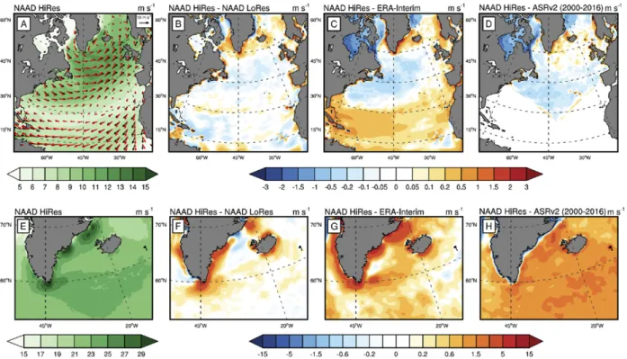
Figure 3 shows the evaluation of climatological winter winds in NAAD HiRes and LoRes. NAAD HiRes and LoRes surface winds are consistent south of 458N with the differences within 60.15 m s21. At
the same time, in the Irminger Sea NAAD HiRes shows stronger mean winds by 0.2–0.6 m s21, thus likely reflecting a better representation of the meso-scale features such as tip jets and katabatic winds in this area. The comparison with ERA-Interim (Fig. 3c) shows stronger trade winds in the NAAD HiRes experiment, somewhat lower wind speeds in the western midlatitude North Atlantic, and also stronger winds in the subpolar North Atlantic along the eastern Greenland coast. North of 408N, differences between HiRes and ASRv2 (Fig. 3d) are consistent with
those for ERA-Interim. Dukhovskoy et al. (2017) noted differences between high-resolution satellite wind products and reanalyses attributing them to the subsynoptic and mesoscale processes. The impact of high-resolution and nonhydrostatic setting onto the wind field is especially evident for extreme winds (Figs. 3e–h). We note much stronger katabatic winds and tip jets along the Greenland coast, with the dif-ferences in surface winds between HiRes and LoRes experiments being locally over 4 m s21 (about 20% of mean values of 99th percentile of wind speed). Relative to ERA-Interim, the HiRes experiment shows extreme winds stronger by more than 7 m s21. Important is that HiRes also shows much better localization of kata-batic winds near the coast in HiRes compared to LoRes and ERA-Interim.Figure 3dshows the local-ization of maximum extreme winds much closer to the Greenland coast in agreement with the case studies (Moore and Renfrew 2005;Moore et al. 2015). Extreme wind speed differences between NAAD HiRes and ASRv2 in the Irminger Sea (Fig. 3h) amount to 1.5– 2 m s21. Comparison of NAAD winds with QuikSCAT winds (Ricciardulli and Wentz 2015) (Fig. 4) indicates that both NAAD HiRes and LoRes have considerably
FIG. 3. (a) January mean (1979–2018) scalar 10-m wind speed (colors) in NAAD HiRes and wind vectors in NAAD HiRes (red) and ERA-Interim (black), along with differences in 10-m wind speed (b) between NAAD HiRes and LoRes, (c) between NAAD HiRes and ERA-Interim, and (d) between NAAD HiRes and ASRv2. Also shown is (e) the January 99th percentile of 10-m wind speed over subpolar North Atlantic in NAAD HiRes and differences in 99th percentile of 10-m wind speed (f) between NAAD HiRes and LoRes, (g) between NAAD HiRes and ERA-Interim, and (h) between NAAD HiRes and ASRv2. For LoRes and ERA-Interim, the differences are shown for the period of 1979–2018; for ASRv2, differences are shown for the period of 2000–16.
smaller errors with respect to QuikSCAT when com-pared with ERA-Interim, which clearly demonstrates a systematic negative bias of 0.5–2 m s21.
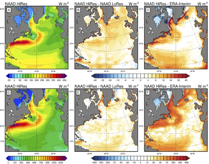
Surface turbulent fluxes (sensible plus latent,Fig. 5) in NAAD HiRes show the structure to be consistent with reanalyses and blended climatologies such as OA-FLUX (e.g.,Yu and Weller 2007) with the locally strong fluxes over the Gulf Stream (primarily due to latent heat) and in the Labrador Sea (mostly due to sensible heat). NAAD HiRes turbulent fluxes are generally larger than those of NAAD LoRes by 0–10 W m22in the open ocean regions and by;30 W m22 over the Gulf Stream and in the Labrador and Irminger Seas. In the subpolar latitudes, the stronger HiRes fluxes are explained by the differences in wind speed (Fig. 3) with a significant contribution from surface temperature and humidity gradients, especially for sensible heat flux (no figure shown). In the midlatitudes and subtropics, the differences in turbulent heat fluxes between HiRes and LoRes are associated with surface temperature and humidity vertical gradients, as wind speed differences here are close to zero (Fig. 3). Differences with ERA-Interim (Fig. 5c) are 30%–50% larger than those with NAAD LoRes, while the direct comparison here is difficult because of the differences between the ERA-Interim surface flux algorithm and the COARE 3.0 flux algorithm (Fairall et al. 2003) used in NAAD (Brodeau et al. 2017). Of interest is also the evaluation of extreme surface turbulent fluxes, which might be strongly de-pendent on mesoscale processes (Ma et al. 2015) and demonstrate differences between different products not consistent with those for mean values (Gulev and Belyaev 2012; Bentamy et al. 2017). Figures 5d–f presents extreme fluxes quantified by the 99th per-centile of the modified Fisher–Tippett distribution (Gulev and Belyaev 2012). Relative to LoRes, HiRes shows stronger extreme fluxes over the Gulf Stream
and the North Atlantic Current where differences may locally exceed 30 W m22(up to 5%–10% of the mean values). In the Irminger Sea the differences amount to 200 W m22, being more than 20%–25% of the mean values of extreme turbulent fluxes. Extreme fluxes diagnosed by HiRes are also considerably stronger than in ERA-Interim (Fig. 5f), with maxi-mum differences locally exceeding 300 W m22. b. Storm tracks and cyclone dynamics
NAAD opens a new avenue in the analysis of cyclone dynamics and storm tracks. Cyclone tracks were diag-nosed using the IORAS algorithm (Zolina and Gulev 2002;Tilinina et al. 2013), tested within the IMILAST project (Neu et al. 2013). Tracking was performed on the NAAD HiRes grid. For tracking cyclones in the limited area over the North Atlantic we applied an approach that accounts for the so-called entry–exit uncertainties (Tilinina et al. 2014). Postprocessing was further applied to cutoff cyclones with migration dis-tances smaller than 1000 km and lifetimes shorter than 24 h (Tilinina et al. 2013).
NAAD HiRes (Fig. 6a) captures well the main North Atlantic storm tracks that are consistent with cyclone climatologies based on the global reanalyses (e.g., Neu et al. 2013; Tilinina et al. 2013). NAAD HiRes shows 30%–60% larger local cyclone numbers compared to LoRes. Also, NAAD LoRes shows slightly larger number of cyclones compared to ERA-Interim while the differences are within 3%–5%. Over the North Atlantic storm track, the number of cyclones in NAAD HiRes is close to that in ERA5 (Fig. 6d) with slightly larger cyclone counts over the storm formation region in the Northwest Atlantic and slightly smaller counts in the central North Atlantic and the subpolar regions.
Figure 7 shows the winter [December–February (DJF)] time series of the domain integrated number of cyclones with different intensities (quantified by central pressure). NAAD HiRes allows for identifi-cation of;2 times more cyclones compared to LoRes, which indicates a high consistency with the global reanalyses, except for ERA5, which reveals practi-cally the same number of cyclones as NAAD HiRes (Fig. 7a). Importantly, these differences between HiRes and all other products (including LoRes) are formed mostly by moderately deep and shallow cy-clones (Figs. 7b,d). At the same time, the number of deep cyclones in HiRes is more consistent with LoRes and reanalyses showing 10%–15% higher counts. Overall, the winter cyclone activity in NAAD is very close to that in ERA5 and considerably more intense compared to the other reanalyses. Summer results
FIG. 4. Histograms of the differences between NAAD HiRes (red), NAAD LoRes (orange), and ERA-Interim (blue) winds with respect to QuikSCAT winds for 2005.
(not shown) are qualitatively similar with even higher differences especially for shallow cyclones dominat-ing durdominat-ing the warm season.
Figure 6 demonstrates relatively strong differences between cyclone counts in NAAD and in all reanalyses over the North American continent. This is likely asso-ciated with the fact that the finer-resolution NAAD HiRes is capable of identifying cyclone generation events at an earlier stage than the global reanalyses. Our analysis of cyclogenesis events (not shown) demon-strates considerably larger counts of cyclone generation events over the North American storm track in NAAD when compared with even ERA5, while the total num-ber of tracks is close in both products (Fig. 7). Also, we note that the cyclone effective radius, characterizing cyclone size (Rudeva and Gulev 2007) is smaller in
NAAD HiRes by about 50–100 km as compared with NAAD LoRes and is also smaller by 100–150 km rela-tive to ERA-Interim (no figure shown). NAAD HiRes also demonstrates capabilities in capturing characteris-tics of extreme cyclones. Thus, our analysis of extremely deep cyclones shows that the 100 deepest cyclones in NAAD HiRes have a central pressure about 4 hPa lower than those in LoRes and ERA-Interim. Similar con-clusions were drawn from WRF-based high-resolution ASR in comparison with global reanalyses (Tilinina et al. 2014).
c. Hydrological cycle
Evaluation of the North Atlantic hydrological cycle in the NAAD is of special interest.Figure 8ashows time series of annual mean precipitation over the NAAD
FIG. 5. (a) January (1979–2018) sensible plus latent turbulent heat fluxes in NAAD HiRes and differences in sensible plus latent turbulent heat flux (b) between NAAD HiRes and LoRes and (c) between NAAD HiRes and ERA-Interim. Also shown is the (d) January (1979–2018) 99th percentile of sensible plus latent turbulent heat flux in NAAD HiRes and differences in 99th percentile of sensible plus latent turbulent heat flux (e) between NAAD HiRes and LoRes and (f) between NAAD HiRes and ERA-Interim.
domain as computed from NAAD HiRes and LoRes experiments, as well as from ERA-Interim, the Global Precipitation Climatology Project (GPCP1DD) (Huffman et al. 2001), and, starting from 2013, the Global Precipitation Measurement (GPM) mission (Skofronick-Jackson et al. 2017). NAAD HiRes shows slightly higher domain integrated total precipitation values compared to NAAD LoRes before the early 2000s and slightly smaller precipitation during the last 15 years. Both HiRes and LoRes domain integrated values are 4%–7% less than ERA-Interim and 5%–10% less than GPCP. Starting from
2013, NAAD HiRes is in a very good agreement with GPM, demonstrating very small (relative to the other products) differences for all seasons (Fig. 8b). The consistency with GPM is, however, somewhat better in autumn–winter than in spring–summer, likely because of a stronger contribution of the convective precipi-tation (requiring even higher resolution than that in HiRes) during the warm season.
Figures 9a–c shows annual mean total precipitation in NAAD HiRes and the differences with LoRes and ERA-Interim. NAAD HiRes when compared with
FIG. 6. (a) Winter (DJF; 1979–2018) number of cyclones in NAAD HiRes and the differences in the DJF number of cyclones (b) between NAAD LoRes and Interim, (c) between NAAD HiRes and ERA-Interim, and (d) between NAAD HiRes and ERA5. Units are cyclone tracks per season (DJF) per circle with a radius of 28 latitude [equivalent to approximately 155 000 km2; seeTilinina et al. (2013,2014)for the mapping metrics].
LoRes shows stronger precipitation in the western Atlantic tropics and over the Gulf Stream by up to 1 mm day21and lower, by 0.3–0.5 mm day21, precip-itation in the North Atlantic subpolar gyre. Relative to ERA-Interim (Fig. 9c), NAAD HiRes shows stronger precipitation over the Gulf Stream (up to 2 mm day21) and weaker precipitation over the subpolar latitudes. The precipitable water content (PWC) (Figs. 9d,e) is lower in NAAD HiRes than in LoRes by 4%–6%, with the strongest absolute differences in the western tropics. ERA-Interim, however, shows a slightly higher PWC than NAAD HiRes over most of the domain except for the western tropics and subtropics (Fig. 9e). Differences in precipitation and PWC suggest stronger tropical water recycling in NAAD HiRes and somewhat weaker recycling in mid- and subpolar latitudes relative to LoRes and ERA-Interim.
Representation of summer precipitation over the western North Atlantic is important for quantifying the lower-atmosphere responses to the ocean frontal signals in the Gulf Stream (Minobe et al. 2008, 2010; Parfitt et al. 2016). Precipitation responses in summer are
typically associated with convective processes and mostly located over the westernmost part of the Gulf Stream. In winter, precipitation responses are associated with the atmospheric frontal activity and enhanced pre-cipitation over the central and eastern Gulf Stream proper (Minobe et al. 2010).Figure 10demonstrates precipitation for July 2015 as revealed by NAAD HiRes and LoRes as well as by ERA-Interim, ERA5, GPM, and GPCP. NAAD HiRes with its capability to capture convective processes shows the best agreement with GPCP in the structure of precipitation pattern and in magnitude. NAAD LoRes and ERA-Interim tend to underestimate precipitation rates by 2–4 and 3–6 mm day21, respectively. ERA5 is most consistent with HiRes in spatial structure but shows smaller precipitation rates of 2–3 mm day21. Comparison with ASRv2 (no figure shown) is somewhat difficult as the ASR domain boundary cuts a considerable part of the region analyzed. However, for the overlapping part of the domain the precipitation pattern in ASRv2 is comparable in structure to that of NAAD HiRes.
Capabilities of the high-resolution NAAD in repre-senting moisture transports can be analyzed through the
FIG. 7. Time series of the seasonal (DJF) (a) total number of cyclones, as well as numbers of (b) moderately deep, (c) deep, and (d) shallow cyclones in NAAD HiRes, NAAD LoRes, and different reanalyses. Thin lines show winter (DJF) annual values, and thick lines show 5-yr running means.
diagnostics of ARs (Lavers and Villarini 2015; Ralph et al. 2017; Shields et al. 2018), representing narrow synoptic-scale jets transporting an abundant amount of water vapor from the ocean to the continents. ARs may be responsible for more than 90% of poleward mois-ture transport (Zhu and Newell 1998) and also result in extreme precipitation events over continental coastal areas (Viale and Nuñez 2011; Lavers and Villarini 2015;Gershunov et al. 2017;Waliser and Guan 2017).
For the detection of ARs, we used the 85th percentile of the integrated water vapor transport (IVT) along with a fixed lower IVT limit of 100 kg m21s21(Guan and Waliser 2015). The 85th percentile of IVT was computed from the 20-day sliding windows in the NAAD-HiRes and LoRes outputs, and moisture transports were computed according toDufour et al. (2016).Figure 11shows the case study for 5 December 2015, with an AR associated with the deep cyclone east of Iceland and clearly seen in IVT fields. Associated daily accumulated precipitation in the NAAD HiRes closely matches that diagnosed by GPM, while, for example, ERA-Interim shows the shift in the location of the AR with respect to GPM. NAAD HiRes precipitation in the AR landfall areas over the U.K. and Norway coasts is over 66 mm day21. This is greater than the values diag-nosed by NAAD LoRes and ERA-Interim by up to 30 mm day21(Fig. 11f). We also note an accurate location of the coastal precipitation maxima in the landfall areas in NAAD HiRes (Fig. 11f). The maximum of water vapor transport in the AR (Fig. 12a) at 2.5-km height is associated with locally strong winds amounting to more than 40 m s21. Figure 12bshows that the AR core in HiRes is character-ized by 10%–15% stronger transports relative to LoRes,
reflecting the fact that ARs in the HiRes experiment are narrower. In climatological context, this reduces the time during which western Europe coasts are exposed to ARs; however, this makes the impact of individual ARs stronger and highly localized. Our estimate for 2015, performed using a method similar toGuan and Waliser (2015), shows that AR landfalls in HiRes happen during 10%–15% of the time, which is less than in LoRes and MERRA (15%–20%).
d. Mesoscale features
To demonstrate the representation of mesoscale fea-tures in the NAAD, we use kinetic energy (KE) wave-number spectra (SKE) derived from the wind speed data and averaged over the layer between 3- and 5-km height over the whole domain (Figs. 13a,b). These spectra characterize the atmospheric turbulence at different scales by the power law SKE(k); k2g, where k is the wave-number and g is changing from approximately 23 to approximately 25/3 between the ranges of space scales larger and smaller than 500 km (Waite and Snyder 2009; Condron and Renfrew 2013; Dukhovskoy et al. 2017). Figure 13demonstrates marked differences in the wave-number spectra for HiRes and LoRes experiments. For the total and geostrophic KE, the HiRes spectrum is better matching k23than LoRes is. It is important, however, that the spectral decay rate for both geostrophic and ageo-strophic components at smaller scales (,500 km) is con-siderably smaller in HiRes than in LoRes. This reflects stronger pressure gradients (and, thus, stronger winds) in synoptic and mesoscale transients in the HiRes experi-ment.Dukhovskoy et al. (2017)noted a similar tendency in
FIG. 8. Time series of the (a) annual mean domain-averaged precipitation (mm day21) for 1979–2017 and (b) monthly mean domain-averaged precipitation (mm day21) for 2014–17 in NAAD HiRes (red), NAAD LoRes (orange), ERA-Interim (blue), ERA5 (cyan), GPCP (green), and GPM (magenta).
ASR relative to global coarser-resolution reanalyses in the subpolar North Atlantic.
Figure 13c shows the wavenumber kinetic energy spectra near the surface using data from NAAD HiRes and ASRv2 over the overlapping part of the two domains. As in the case of the free troposphere (Figs. 13a,b), the NAAD HiRes spectrum built from the surface data closely matches k25/3decay rate in the range of scales less than 700 km. The ASRv2 spectrum demonstrates a very similar behavior in terms of change in g from;23 to ;25/3 and the decay rate in the range from 700 to at least 100–150 km.
In this respect it is of interest to consider the repre-sentation of polar lows in NAAD. Polar lows represent highly localized maritime atmospheric phenomena as-sociated with extreme winds and advection of very dry cold air, playing an important role in high-latitude at-mospheric dynamics and air–sea interaction processes (Zahn and von Storch 2008; Condron et al. 2008; Condron and Renfrew 2013, among others). They are
hardly detectable in global reanalyses primarily due to their small size (Zappa et al. 2014;Stoll et al. 2018). Many publications, however, report the capability of the WRF Model even without data assimilation to ef-fectively simulate polar lows (Wagner et al. 2011;Wu et al. 2011;Føre et al. 2012;Kolstad et al. 2016).Kolstad (2011) developed a unique database of 63 polar lows (1999–2009) in the subpolar and subarctic North Atlantic and Arctic using AVHRR and QuikSCAT winds. Of the 21 events identified by Kolstad (2011) in the NAAD domain, NAAD HiRes was able to successfully detect 20 polar lows.
Figure 14shows a case study for the polar low that developed on 2 March 2008 in the Irminger Sea. NAAD HiRes detects well the location of the pressure mini-mum identifying a 978-hPa central pressure, which is deeper than that in ERA-Interim (986 hPa) and even in ERA5 (984 hPa). Also, NAAD HiRes demonstrates the well-detectable comma-type structure not present in ERA-Interim and ERA5 and less evident in ASRv2.
FIG. 9. (a) Annual (1979–2018) mean precipitation (mm day21) in NAAD HiRes and differences in the annual mean precipitation (b) between NAAD HiRes and NAAD LoRes and (c) between NAAD HiRes and ERA-Interim. Also shown are (d) annual (1979–2018) mean atmospheric precipitable water content (kg m22) in NAAD HiRes and differences in the annual mean precipitable water content (e) between NAAD HiRes and NAAD LoRes and (f) between NAAD HiRes and ERA-Interim (f).
Note that NAAD LoRes results (no figure shown) are very close to ERA-Interim for this case. The associated maximum surface wind speed in the polar low amounts in HiRes to 32 m s21, with 26–27 m s21in ERA-Interim and ERA5, and nearly 30 m s21 in ASRv2 (Fig. 14). Note thatGutjahr and Heinemann (2018)clearly dem-onstrated that an accurate representation of the tip jets and associated extreme winds around Greenland re-quires resolutions of at least 15 km. Remarkably, it is also the case that surface turbulent fluxes (sensible plus latent) are considerably stronger in HiRes (up to 900 W m22) than in ERA-Interim (600 W m22) and are comparable to both ERA5 and ASRv2. We note that the direct comparison of surface fluxes between these prod-ucts should be taken with caution because of the use of somewhat different flux algorithms. However, the anal-ysis of surface flux PDFs and the surface flux relative extremeness (Gulev and Belyaev 2012; Tilinina et al. 2018) show that the strong flux event during 2 March 2008 in NAAD HiRes contributed more to the total monthly flux as compared with ERA5 and ASRv2.
The capability of the NAAD to capture the mesoscale dynamics in the tropics is evaluated inFig. 13dshowing wavenumber spectra of the kinetic energy near the surface (10 m) and at 1500 m in HiRes and LoRes sim-ulations. Remarkably, the spectra near the surface and at 1500 m are qualitatively close to each other for both simulations and are also close to the spectra for the free
troposphere (Figs. 13a,b) and to the surface spectra in the subpolar region (Fig. 13c). At the same time, tropical spectra for HiRes demonstrate a k25/3decay rate for the wave lengths from 200 to 1000 km, while LoRes spectra follow k23 and a slightly stronger decay rate in this range. This implies more energetic mesoscale features of the same size in the tropics in HiRes than in LoRes.
NAAD is also capable of identifying tropical cyclones generated and propagating north of the southern margin of the domain. Figure 15 shows the diagnostics of Hurricane Gaston, which developed over the North Atlantic between 22 August and 2 September 2016. At the moment of maximum development, NAAD HiRes diagnoses the lowest central pressure (6 hPa deeper when compared with ERA5 and more than 15 hPa deeper than NAAD LoRes and ERA-Interim) as well as winds stronger by 5–8 m s21than in ERA5. Associated precipi-tation in NAAD HiRes is considerably stronger than in LoRes and ERA-Interim and consistent in magnitude with ERA5. However, the precipitation pattern in HiRes more accurately captures the shape implied by GPM than ERA5. 5. Pilot ocean applications
a. Effects in modeled ocean circulation
To demonstrate the NAAD capabilities for driving long-term experiments with regional configurations of ocean general circulation models, we developed surface
FIG. 10. July 2015 monthly precipitation rates (mm day21) in (a) NAAD HiRes, (b) LoRes, (c) ERA-Interim, (d) GPM, (e) GPCP, and (f) ERA5.
forcing functions for the ocean based upon NAAD HiRes and NAAD LoRes and used them to drive a northern North Atlantic regional configuration of the NEMO (version 3.6) ocean and sea ice general circula-tion model (Madec et al. 2016). This configuracircula-tion (re-ferred to as NNATL12) covers the subpolar gyre of the North Atlantic (Verezemskaya et al. 2020, manuscript submitted to J. Geophys. Res.) at a resolution of ap-proximately 4.5 km. The model configuration setup in-cluding configuration geometry (1/128 grid, 75 vertical z levels with fine separation (1 m) near the surface, coast-lines, and bathymetry), numerical schemes and physical process parameterizations are those commonly used for the global 1/128 eddy-resolving global ocean circulation model ORCA12 for the operational forecasts (Lellouche
et al. 2018) as well as for climate-oriented long-term simulations (e.g., Sérazin et al. 2018; Hewitt et al. 2016) and process studies (e.g.,Akuetevi et al. 2016). At the open northern and southern boundaries as well as at the western boundary of Hudson Bay, the model is driven by monthly mean temperature, salinity, ve-locity, and sea ice from the Global Ocean Reanalysis Simulation (GLORYS12), version 4 (v4) (Garric and Parent 2018). The model was tested in a set of sensi-tivity experiments and validated against the high-resolution the 1/128 GLORYS12 reanalysis of the Copernicus Marine Environment Monitoring Service (Fernandez and Lellouche 2018), satellite observa-tions, and repeated full-depth hydrographic sections at 608N (Sarafanov et al. 2012; Gladyshev et al. 2018;
FIG. 11. Representation of AR on 5 Dec 2015: (a) vertically integrated water vapor transport in NAAD HiRes and daily accumulated precipitation diagnosed by (b) GPM, (c) NAAD HiRes, (d) LoRes, and (e) ERA-Interim, along with (f) the difference in precipitation between NAAD HiRes and ERA-Interim over the area of AR landfall. The zoomed-in area in (f) is shown by the black-outlined box in (c). Line AB in (a) shows the cross section displayed inFig. 12, below.
Verezemskaya et al. 2020, manuscript submitted to J. Geophys. Res.).
Comparative model experiments were performed with NAAD HiRes and NAAD LoRes atmospheric forcings; the experiments are referred to as NAAD-OHR and NAAD-OLR, respectively. Significant differences in characteristics of turbulent and radiative heat fluxes as well as momentum fluxes between the two forcings at the ocean surface result in large differences in the sim-ulated ocean mean state. Thus, the domain-averaged simulated SST is approximately 0.68C lower in NAAD-OHR, with summer differences amounting to more than 1.58C (Fig. 16), in close agreement with European Space Agency (ESA) SST (http://www.esa-sst-cci.org). Note that trends in SST are highly consistent in both NAAD-OHR and NAAD-OLR. The strongest SST negative differences of 18–1.58C and lower sea surface salinity (0.15–0.2 psu) in OHR relative to NAAD-OLR are observed in the Labrador and Irminger Seas. Consistent with SST, NAAD-OHR shows a lower ocean heat content for both the upper (0–700 m) and intermediate ocean (700–1500 m), suggesting a more intense ventilation of the ocean by convective pro-cesses in NAAD-OHR (Fig. 16). Since almost all ocean models in noncoupled experiments have a tendency toward a warmer and saltier ocean (Tréguier et al. 2005;Rattan et al. 2010), the colder upper-ocean tem-peratures in NAAD-OHR should be considered as an improvement. The OHR forcing also appears to drive significant changes in the boundary currents around Greenland and in the different branches of the central North Atlantic Current, which were found to be more
intense and more variable in NAAD-OHR than in NAAD-OLR, as revealed by the partition of eddy ki-netic energy (not shown). NAAD-OHR also shows a somewhat deeper mixed layer depth (MLD) relative to NAAD-OLR (not shown) in regions known for being strongly ventilated by winter convection (the southwest sector of the Labrador Sea and the central Irminger Sea). A lesser ventilation is noticed in the areas where ocean eddies are known to counterbalance the effects of strong surface fluxes onto MLD (e.g.,Chanut et al. 2008). b. Effects in ocean wind-wave modeling
NAAD can be also effectively used for forcing spec-tral wave models whose solutions are critically depen-dent on the quality and spatial resolution of atmospheric forcing (Cavaleri 2009;Ardhuin et al. 2012). In this re-spect, the mesoscale activity in the lower atmosphere might be of critical importance for capturing extreme wind waves (Condron et al. 2006; Zappa et al. 2014; Markina et al. 2019).
We used NAAD HiRes and LoRes outputs for the WAVEWATCH III spectral wave model (WW3DG 2016) over the NAAD domain. Experiments (referred to as NAAD-WHR and NAAD-WLR for HiRes and LoRes forcing, respectively) were performed with the spatial resolution of 0.28 and spectral model resolution being 36 directions and 25 frequencies spanning from 0.04 Hz with an increment of 1.1. The WAVEWATCH– III configuration included ST6 parameterization for wave energy input and dissipation (Zieger et al. 2015; Liu et al. 2019) calibrated for WRF winds (Markina et al. 2018) and the ice source term package (IC0; Tolman
FIG. 12. (a) Moisture transport across the AB section (seeFig. 11a) on 5 Dec 2015 in NAAD HiRes (colors) and the component of wind speed orthogonal to the section (contours) as well as (b) the difference in the moisture transport across the AB section on 5 Dec 2015 between NAAD HiRes and NAAD LoRes.
2003) implying the exponential attenuation of waves in partially sea ice–covered regions. To account for the ocean surface current impact on growing waves we used daily surface current velocities from the NEMO-based Ocean Reanalysis System 5 (ORAS5;Zuo et al. 2019). Cavaleri (2009)argued that the increase in spatial res-olution of forcing per se does not necessarily result in the increase in significant wave height (SWH); rather, the formation of high waves is associated with higher winds, changes in the duration of wind action, and the length of fetch. In this sense, NAAD HiRes with its stronger
winds (Fig. 3), smaller cyclone sizes and larger number of synoptic transients (Figs. 5and6) likely acts locally rather than on a larger scale.
Figures 17a and 17b show winter (January–March) climatological SWH for 1979–2018 in NAAD-WHR and the differences between WHR and NAAD-WLR. In NAAD-WHR the highest SWH amounts to 5.4 m in the eastern subpolar North Atlantic in very close agreement with VOS observations (Gulev et al. 2003;Gulev and Grigorieva 2006). Differences between NAAD-WHR and NAAD-WLR SWH over most of the
FIG. 13. Wavenumber kinetic energy spectra derived from wind speed data and averaged over the layer between 3- and 5-km height over the whole NAAD domain for (a) NAAD HiRes and (b) NAAD LoRes. In (a) and (b), spectra for the total (black), geostrophic (green), and ageostrophic (yellow) kinetic energy are shown. Dotted lines show power laws of k23and k25/3, as labeled. (c) Wavenumber kinetic energy spectra derived from surface wind speed diagnosed by NAAD HiRes (green) and ASRv2 (blue) for the area of overlap of the NAAD and ASRv2 domains. The area of overlap of NAAD and ASRv2 is outlined in red in the inlay map, and the gray line in the inlay shows the southern boundary of the ASRv2 domain in the Atlantic region. (d) Wavenumber kinetic energy spectra derived from NAAD HiRes (black) and NAAD LoRes (gray) for the surface (solid lines) and 1500 m (dashed lines) for the tropical domain outlined in red in the inlay map.
North Atlantic midlatitudes and subtropics are gen-erally within 0.3 m but strongly increase in the sub-polar North Atlantic where they amount to 0.8 m in the Irminger Sea. The highest extreme strong waves quantified as 95th percentile amount in winter in NAAD-WHR to 9 m (Fig. 17c), being higher than in NAAD-WLR by 0.2–0.5 m in the central and eastern subpolar North Atlantic (Fig. 17d). At the same time the most distinctive differences between the NAAD-WHR and NAAD-WLR experiments are identified along the southeast Greenland coast where the ex-treme SWH in NAAD-WHR is higher than that in NAAD-WLR by more than 1 m (up to 20% of mean values). This likely reflects a more accurate repre-sentation of katabatic winds and tip jets in this area in NAAD-WHR.
6. Summary and outlook
We presented NAAD—a new 3D multidecadal at-mospheric dataset for the North Atlantic produced with a WRF nonhydrostatic model at mesoscale reso-lution (NAAD HiRes). In parallel, a coarser-resoreso-lution dataset (NAAD LoRes) was produced with a spatial
resolution close to ERA-Interim used in both experi-ments as a lateral boundary condition.
Our evaluation demonstrates reasonably realistic re-presentations of most climatological characteristics in both NAAD HiRes and NAAD LoRes datasets. The main differences are identified in the ice-covered sub-arctic regions, especially for surface air temperature and partly for surface humidity. At the same time, atmo-spheric dynamics was quite adequately represented. The major purpose of the NAAD at this stage was not to provide extremely close comparability of NAAD LoRes with, for example, ERA-Interim. This is hardly achiev-able because ERA-Interim (as well as the other rean-alyses) is largely constrained by data assimilation. The major NAAD focus was rather to develop a high-resolution atmospheric dataset that allows a better analysis of subsynoptic and mesoscale features—the task still not resolved by global reanalyses over the North Atlantic. In this respect, the objectives for NAAD are similar to those posed for the other regional rean-alyses (e.g., ASR; Bromwich et al. 2018). The NAAD model configuration was quite close to the one used in ASR, the lateral conditions are the same (ERA-Interim) and the resolutions of the two products are
FIG. 14. Diagnostics of the polar low on 2 Mar 2008. Shown is the surface 10-m wind speed (colors) and mean sea level pressure (MSLP; contours) as revealed by (a) NAAD HiRes, (b) ERA-Interim, (c) ERA5, and (d) ASRv2. Also shown is sensible plus latent heat flux (colors) and MSLP (contours) diagnosed by (e) NAAD HiRes, (f) ERA-Interim, (g) ERA5, and (h) ASRv2.
similar. At the same time ASR (both ASRv1 and ASRv2) used extensive data assimilation input that ex-ceeds data assimilation in the global reanalysis (e.g., ERA-Interim). Our capabilities for the direct compari-sons of NAAD with ASR were limited to the subpolar latitudes. However, the analysis of kinetic energy spec-tra and extreme winds and fluxes associated with polar lows (Figs. 13 and 14) clearly demonstrated that the differences between NAAD HiRes and ASRv2 are the smallest relative to the other reanalyses, and this is re-assuring. The comparative analysis of surface fluxes, winds, and precipitation in the North Atlantic midlati-tudes is not representative, as these regions are close to the boundary of the ASR domain.
Extensive evaluation of ASR (e.g.,Moore et al. 2015; Bromwich et al. 2016;Tilinina et al. 2014) demonstrated the added value of high-resolution nonhydrostatic model settings in improving the representation of polar lows and tip jets, as well as extratropical cyclones. In this respect,
our comparison of HiRes and LoRes simulations confirms the conclusions drawn from the ASR evaluation. It also clearly demonstrates the added value of high-resolution and nonhydrostatic model settings in NAAD over the whole North Atlantic. Specifically, NAAD HiRes pro-vides the possibility to resolve mesoscale dynamics as-sociated with high winds, first of all in the North Atlantic subpolar latitudes characterized by small-scale polar lows and tip jets. Here NAAD HiRes demonstrated stronger extreme winds and their better localization compared to the LoRes version and modern reanalyses. Much higher resolution of the WRF Model in NAAD HiRes provides a new view of the North Atlantic ex-tratropical cyclone activity with 2 times as large a total number of cyclones counted in NAAD HiRes relative to LoRes and most reanalyses. This difference was pri-marily due to cyclones that are smaller in size and rel-atively shallow, which were poorly simulated in the LoRes experiment and in global reanalyses.
FIG. 15. Diagnostics of Hurricane Gaston in the moment of maximum development on 0000 UTC 31 Aug 2016, showing (a) the pre-cipitation pattern diagnosed by GPM and the MSLP (contours), 10-m wind speed vectors (arrows), and prepre-cipitation (colors) as diagnosed by (b) NAAD HiRes, (c) NAAD LoRes, (d) ERA-Interim, and (e) ERA5.
Higher extreme turbulent fluxes in NAAD HiRes and a better representation of the convective precipi-tation over the Gulf Stream make NAAD potentially useful for quantifying ocean–atmosphere interactions at mesoscales and depicting ocean impacts on the lower atmosphere and associated responses in the dynamics of midlatitude storm tracks. NAAD is also capable of capturing highly localized mechanisms of atmospheric moisture transports such as ARs, more accurately locating them, and quantifying their inten-sity and impacts. In the tropics, NAAD HiRes also effectively captures mesoscale features, including an improved representation of tropical cyclones, espe-cially in terms of central pressure, wind, and precipi-tation. Applications of NAAD to ocean modeling demonstrated the effect of HiRes onto the modeled ocean state and eddy kinetic energy distribution, specifically showing smaller surface temperature and upper-ocean heat content consistently with observa-tions. Being applied to wind-wave modeling, NAAD
HiRes resulted in higher simulated extreme wind waves in the eastern subpolar North Atlantic, reflecting stronger extremeness of surface winds.
Further near-time developments of the NAAD will include the adaptation of ERA5 as a source for lateral boundary conditions and changing to a finer spatial resolution of at least;3 km with a higher number of vertical layers. This will also include at least for the period after 2000 the use of high-resolution SST and sea ice data, available from the Operational Sea Surface Temperature and Sea Ice Analysis (OSTIA) system (Roberts-Jones et al. 2012;Donlon et al. 2012) as well as from Multisensor Analyzed Sea Ice Extent (MASIE) AMSR2 (MASAM2;Fetterer et al. 2015). Improved representation of sea ice will help to min-imize biases in temperature and humidity in the northern North Atlantic. Also planned is the domain extension to the full coverage of the North Atlantic tropics that will make it possible to provide accurate diagnostics of tropical cyclone dynamics including
FIG. 16. (top) Domain-averaged simulated ocean SST in NAAD-OHR (orange) and NAAD-OLR (magenta), along with ESA SST (green). Time series of ESA SST are shown only for the period of data availability (1993–2010). (bottom) Domain-averaged ocean heat content for the 0–700-m layer (upper curves) and the 700–1500-m layer (lower curves) in NAAD-OHR (orange) and NAAD-OLR (magenta). The inlay map shows the domain of the NNATL12 ocean general circulation model. Thick lines in the bottom panels show monthly means, and dashed lines show annual means.
the poleward shift in the trajectories (Studholme and Gulev 2018;Sharmila and Walsh 2018). Finer spatial and vertical resolution will also provide a better representation of mesoscale features and will better demonstrate the value added by nonhydrostatic model configurations. For selected years (provisionally in the 2010s), we are also planning to develop ensemble simulations (up to 10 members). In parallel, on a midterm scale we will work on the transition of NAAD to the North Atlantic regional reanalysis with assimilating all available information over the do-main that will make it possible to develop the product for assessing the impact of mesoscale processes onto
longer-term climate variability in the atmosphere and the ocean.
Acknowledgments. We acknowledge the support by the Russian Academy of Sciences (ST-ASS-0149-2018-0001) and the Ministry of Science and Higher Education of Russian Federation under the Agreement 14.W0331.0006. Authors Tilinina and Markina were also supported by Grant 17-77-20112 from the Russian Science Foundation. The analysis of the hydrological cycle (authors Zolina, Dufour, and Krinitskiy) benefited from Helmholtz-RSF Grant 18-47-06202. We greatly appreciate critically im-portant comments of the two anonymous reviewers and
FIG. 17. (a) Mean SWH in NAAD-WHR and (b) difference in the mean SWH between NAAD-WHR and NAAD-WLR over the period of 1979–2018, as well as (c) mean 95th percentile of SWH in NAAD-WHR and (d) difference in 95th percentile of SWH between NAAD-WHR and NAAD-WLR.
the editor. Their insightful suggestions helped to largely improve the first version of the paper. We thank Peter Koltermann of MSU for useful comments on the paper text. Our analysis of mesoscale dynamics was strongly motivated by Peter Arseev of PhIRAS and Alexey Morozov of ITEP. Discussions on the model setting with Andrey Glazunov of INMRAS are appreciated. We ac-knowledge the access to the facilities of HPC computing resources at Lomonosov Moscow State University as well as support of the IORAS administration and RSC-Technologies Group in maintaining supercom-puters and data storage systems at IORAS.
REFERENCES
Akuetevi, C. Q. C., B. Barnier, J. Verron, J.-M. Molines, and A. Lecointre, 2016: Interactions between the Somali current eddies during the summer monsoon: Insights from a numerical study. Ocean Sci., 12, 185–205, https://doi.org/10.5194/os-12-185-2016 https://doi.org/10.5194/OS-12-https://doi.org/10.5194/os-12-185-2016.
Ardhuin, F., and Coauthors, 2012: Numerical wave modeling in conditions with strong currents: Dissipation, refraction, and relative wind. J. Phys. Oceanogr., 42, 2101–2120, https:// doi.org/10.1175/JPO-D-11-0220.1.
Behrens, E., K. Våge, B. Harden, A. Biastoch, and C. W. Böning, 2017: Composition and variability of the Denmark Strait Overflow Water in a high-resolution numerical model hind-cast simulation. J. Geophys. Res. Oceans, 122, 2830–2846,
https://doi.org/10.1002/2016JC012158.
Bentamy, A., and Coauthors, 2017: Review and assessment of la-tent and sensible heat flux accuracy over the global oceans. Remote Sens. Environ., 201, 196–218,https://doi.org/10.1016/ j.rse.2017.08.016 https://doi.org/10.1016/J.RSE.2017.08.016. Bishop, S. P., R. J. Small, F. O. Bryan, and R. A. Tomas, 2017: Scale
dependence of midlatitude air–sea interaction. J. Climate, 30, 8207–8221,https://doi.org/10.1175/JCLI-D-17-0159.1. Boisvert, L. N., M. A. Webster, A. A. Petty, T. Markus, D. H.
Bromwich, and R. I. Cullather, 2018: Intercomparison of precipitation estimates over the Arctic Ocean and its periph-eral seas from reanalyses. J. Climate, 31, 8441–8462,https:// doi.org/10.1175/JCLI-D-18-0125.1.
Bond, N. A., and M. F. Cronin, 2008: Regional weather patterns during anomalous air–sea fluxes at the Kuroshio Extension Observatory (KEO). J. Climate, 21, 1680–1697,https://doi.org/ 10.1175/2007JCLI1797.1.
Brodeau, L., B. Barnier, A.-M. Treguier, T. Penduff, and S. Gulev, 2010: An ERA40-based atmospheric forcing for global ocean circulation models. Ocean Modell., 31, 88–104,https://doi.org/ 10.1016/j.ocemod.2009.10.005.
——, ——, S. K. Gulev, and C. Woods, 2017: Climatologically significant effects of some approximations in the bulk pa-rameterizations of turbulent air–sea fluxes. J. Phys. Oceanogr., 47, 5–28,https://doi.org/10.1175/JPO-D-16-0169.1.
Bromwich, D. H., K. M. Hines, and L.-S. Bai, 2009: Development and testing of Polar Weather Research and Forecasting model: 2. Arctic Ocean. J. Geophys. Res., 114, D08122,https:// doi.org/10.1029/2008JD010300.
——, A. B. Wilson, L. Bai, G. W. Moore, and P. Bauer, 2016: A comparison of the regional Arctic System Reanalysis and the global ERA-Interim reanalysis for the Arctic. Quart. J. Roy.
Meteor. Soc., 142, 644–658,https://doi.org/10.1002/qj.2527 https:// doi.org/10.1002/QJ.2527.
——, and Coauthors, 2018: The Arctic System Reanalysis, version 2. Bull. Amer. Meteor. Soc., 99, 805–828, https://doi.org/ 10.1175/BAMS-D-16-0215.1.
Bukovsky, M. S., and D. J. Karoly, 2009: Precipitation simula-tions using WRF as a nested regional climate model. J. Appl. Meteor. Climatol., 48, 2152–2159, https://doi.org/10.1175/ 2009JAMC2186.1.
Cavaleri, L., 2009: Wave modeling—Missing the peaks. J. Phys. Oceanogr., 39, 2757–2778,https://doi.org/10.1175/2009JPO4067.1. Chanut, J., B. Barnier, W. Large, L. Debreu, T. Penduff, J.-M. Molines, and P. Mathiot, 2008: Mesoscale eddies in the Labrador Sea and their contribution to convection and re-stratification. J. Phys. Oceanogr., 38, 1617–1643, https:// doi.org/10.1175/2008JPO3485.1.
Chao, Y., Z. Li, J. D. Farrara, and P. Hung, 2009: Blending sea surface temperatures from multiple satellites and in situ ob-servations for coastal oceans. J. Atmos. Oceanic Technol., 26, 1415–1426,https://doi.org/10.1175/2009JTECHO592.1. Chassignet, E. P., and X. Xu, 2017: Impact of horizontal resolution
(1/128 to 1/508) on Gulf Stream separation, penetration, and variability. J. Phys. Oceanogr., 47, 1999–2021,https://doi.org/ 10.1175/JPO-D-17-0031.1.
Chelton, D. B., and F. J. Wentz, 2005: Global microwave sat-ellite observations of sea surface temperature for numer-ical weather prediction and climate research. Bull. Amer. Meteor. Soc., 86, 1097–1116, https://doi.org/10.1175/BAMS-86-8-1097.
Chen, F., and J. Dudhia, 2001: Coupling an advanced land surface–hydrology model with the Penn State–NCAR MM5 modeling system. Part I: Model implementation and sensi-tivity. Mon. Wea. Rev., 129, 569–585,https://doi.org/10.1175/ 1520-0493(2001)129,0569:CAALSH.2.0.CO;2.
Condron, A., and I. A. Renfrew, 2013: The impact of polar meso-scale storms on northeast Atlantic Ocean circulation. Nat. Geosci., 6, 34–37, https://doi.org/10.1038/ngeo1661 https:// doi.org/10.1038/NGEO1661.
——, G. R. Bigg, and I. Renfrew, 2006: Polar mesoscale cyclones in the northeast Atlantic: Comparing climatologies from ERA-40 and satellite imagery. Mon. Wea. Rev., 134, 1518–1533,
https://doi.org/10.1175/MWR3136.1.
——, ——, and I. A. Renfrew, 2008: Modeling the impact of polar mesocyclones on ocean circulation. J. Geophys. Res. Oceans, 113, C10005,https://doi.org/10.1029/2007JC004599.
Copernicus Climate Change Service, 2017: ERA5 hourly data on single levels from 1979 to present. Copernicus Climate Change Service Climate Data Store, accessed 23 August 2019,https:// doi.org/10.24381/cds.adbb2d47.
Danabasoglu, G., and Coauthors, 2014: North Atlantic simula-tions in Coordinated Ocean-Ice Reference Experiments phase II (CORE-II). Part I: Mean states. Ocean Modell., 73, 76–107,https://doi.org/10.1016/j.ocemod.2013.10.005 https:// doi.org/10.1016/J.OCEMOD.2013.10.005.
——, and Coauthors, 2016: North Atlantic simulations in Coordinated Ocean-Ice Reference Experiments phase II (CORE-II). Part II: Inter-annual to decadal variability. Ocean Modell., 97, 65–90,https://doi.org/10.1016/j.ocemod.2015.11.007 https:// doi.org/10.1016/J.OCEMOD.2015.11.007.
Dee, D. P., and Coauthors, 2011: The ERA-Interim reanalysis: Configuration and performance of the data assimilation sys-tem. Quart. J. Roy. Meteor. Soc., 137, 553–597,https://doi.org/ 10.1002/qj.828 https://doi.org/10.1002/QJ.828.
![Figure 7 shows the winter [December–February (DJF)] time series of the domain integrated number of cyclones with different intensities (quantified by central pressure)](https://thumb-eu.123doks.com/thumbv2/123doknet/13610697.424747/8.850.80.418.94.280/december-february-integrated-cyclones-different-intensities-quantified-pressure.webp)