Domain adaptation via dimensionality reduction for the comparison of cardiac simulation models

(1)

HAL Id: hal-02154942

https://hal.archives-ouvertes.fr/hal-02154942

Submitted on 13 Jun 2019

HAL is a multi-disciplinary open access

archive for the deposit and dissemination of

sci-entific research documents, whether they are

pub-lished or not. The documents may come from

teaching and research institutions in France or

abroad, or from public or private research centers.

L’archive ouverte pluridisciplinaire HAL, est

destinée au dépôt et à la diffusion de documents

scientifiques de niveau recherche, publiés ou non,

émanant des établissements d’enseignement et de

recherche français ou étrangers, des laboratoires

publics ou privés.

Domain adaptation via dimensionality reduction for the

comparison of cardiac simulation models

Nicolas Duchateau, Kenny Rumindo, Patrick Clarysse

To cite this version:

Nicolas Duchateau, Kenny Rumindo, Patrick Clarysse. Domain adaptation via dimensionality

reduc-tion for the comparison of cardiac simulareduc-tion models. 10th Internareduc-tional Conference on Funcreduc-tional

Imaging and Modeling of the Heart (FIMH 2019), 2019, Bordeaux, France.

�10.1007/978-3-030-21949-9_30�. �hal-02154942�

(2)

for the comparison of cardiac simulation models

Nicolas Duchateau1_{, Kenny Rumindo}1_{, and Patrick Clarysse}1

Creatis, CNRS UMR5220, INSERM U1206, Universit´e Lyon 1, INSA Lyon, France.

Abstract. We tackle the determination of a relevant data space to quan-tify differences between two databases coming from different sources. In the present paper, we propose to quantify differences between cardiac simulations from two different biomechanical models, assessed through myocardial deformation patterns. At stake is the evaluation of a given model with respect to another one, and the potential correction of bias necessary to merge two databases. We address this from a domain adap-tation perspective. We first represent the data using non-linear dimen-sionality reduction on each database. Then, we formulate the mapping between databases using cases that are shared between the two databases: either as a linear change of basis derived from the learnt eigenvectors, or as a non-linear regression based on the low-dimensional coordinates from each database. We demonstrate these concepts by examining the principal variations in deformation patterns obtained from two cardiac biomechanical models personalized to 20 and 15 real healthy cases, re-spectively, from which 11 cases were simulated with both models.

1 Introduction

Simulations stand as a powerful support to understand complex physiological phenomena, and as a potential way to enrich real databases with large amounts of realistic data [1, 2]. However, strong differences may exist between the simu-lations obtained from distinct models, and between simulated and real data. For cardiac biomechanical models, personalization often focuses on matching global parameters such as volumes or pressures [3], although some works went further by matching finer traits such as myocardial deformation patterns [4, 5].

Nonetheless, matching the data from different but comparable sources can be performed a-posteriori, and falls under the umbrella of domain adaptation tech-niques [6, 7]. Simple examples in medical imaging include the global adaptation of data distributions, illustrated on real cardiac meshes from different magnetic resonance protocols [8] or real vs. simulated fluoroscopy images to train a trans-ducer localization algorithm [1]. The merging of databases can be made more sample-specific after reducing the dimensionality of the data. Recent works in-vestigated the estimation of joint spaces that merge heterogeneous data features [9, 10]. We are more interested in adapting the data from one database to an-other one, as pursued globally in [8, 1]. A mathematically sound framework for

(3)

2 N. Duchateau et al.

Population Model

#1

20 healthy cases processed as in [13]: - 11 cases from cMAC-STACOM 2011 [12], - 9 cases from our clinical collaborators.

Left ventricular segmentations from CVI42 software1.

- hexahedral elements - finite elements model - ABAQUS software2

#2

15 healthy cases processed as in [2], all from cMAC-STACOM 2011 [12].

Biventricular segmentations from a statistical atlas.

- tetrahedral elements - finite elements model - SOFA framework3 Table 1: Summary of populations and models used, with 11 cases shared between the two populations and simulated with both models.

1_{https://www.circlecvi.com/cardiac-mri/}

2_{https://www.3ds.com/products-services/simulia/products/abaqus/}

3_{https://www.sofa-framework.org/}

this was developed in [11] with diffusion maps, a spectral embedding technique relevant for clustered data samples.

Here, we demonstrate the interest of this strategy to quantify differences between cardiac simulations from two different biomechanical models, assessed through myocardial deformation patterns. Such simulations build upon different input segmentations, modeling strategies, and personalization. We specifically explore linear and non-linear ways to formulate correspondences between the two populations and therefore to perform domain adaptation, and benchmark them against simple data mapping using mesh registration.

2 Methods

2.1 Data and pre-processing

We processed healthy left ventricular deformation patterns generated using two distinct cardiac biomechanical models personalized to two different populations, as summarized in Tab.1. Population #2 consists of all the cases from the cMAC-STACOM 2011 challenge [12]. Population #1 consists of 11 of these cases, as the 4 remaining cMAC-STACOM cases could not be loaded to the segmentation software CVI421_{, and 9 other cases from our clinical collaborators at CHU Saint}

Etienne, France. The 11 cases simulated with both models were used to define the mapping between the two databases as described in Sec.2.2. We therefore focused the analysis on myocardial deformation parameters that are common to the output of the two models (radial, circumferential and longitudinal strain).

These data are originally defined on subject-specific meshes, and were matched to a given template for each database before the population analysis (here, an arbitrarily chosen mesh in each population). For population #1, correspondences between meshes were obtained by mesh parameterization along the radial, cir-cumferential, and longitudinal directions taking advantage of the hexahedral elements. For population #2, such parameterization is more challenging due to

(4)

0 40

Population #1

(N=20) Population #2original (N=15) registered (N=15)Population #2 Shared cases 10 5 15 20 0 1 number of dimensions eigenvalue Population #1 (N=20) Population #2 original (N=15) Population #2 registered (N=15)

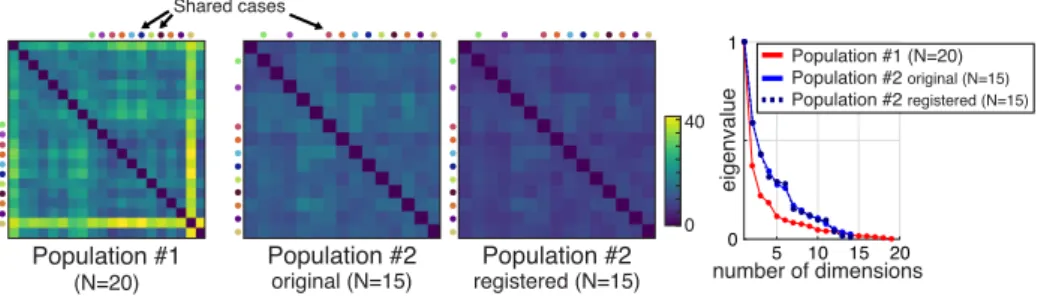
Fig. 1: Left : pairwise comparison of cases in each population, using the Euclidean dis-tance between deformation patterns —treated as column vectors, after concatenating the radial, circumferential and longitudinal components. Colored dots point out the 11 cases shared between the two databases. Right : eigenvalues normalized by the first eigenvalue.

the tetrahedral elements and the biventricular segmentations. Correspondences between meshes were therefore obtained by registering left ventricular surface meshes using the currents representation and the large deformation diffeomor-phic metric mapping framework, with the open-source software Deformetrica [14], and finally propagating the transformation to the left ventricular volumet-ric meshes. For both populations, data from each individual were finally interpo-lated at the cells and vertices of the template mesh using kernel ridge regression and the estimated mesh correspondences as in [13].

A similar pipeline was used to match the template meshes from the two populations, and therefore transport the data from one population to the other without domain adaptation, for benchmarking purposes.

2.2 Dimensionality reduction and domain adaptation

Let’s denote ym,k ∈ Ym the high-dimensional input data associated to subject

k ∈ [1, Km] for the dataset m ∈ {1, 2} (in our case, the deformation patterns

defined over the left ventricular meshes for each individual —treated as column vectors, after concatenating the radial, circumferential and longitudinal compo-nents). For each dataset, standard dimensionality reduction is applied to the Km samples, and provides the low-dimensional coordinates xm,k ∈ Xm. Here,

we tested our methods with the Isomap algorithm [15], a non-linear dimension-ality reduction algorithm that builds a neighborhood graph between the high-dimensional input samples, and looks for a low-high-dimensional space in which the Euclidean distance approximates the geodesic distance in the high-dimensional space.

The small population size may limit the generalization ability of the represen-tation, but may be less critical compared to recently popular techniques such as auto-encoders, which may require larger populations. Also, domain adaptation via dimensionality reduction was thoroughly investigated for the diffusion maps algorithm [11], but this algorithm is more relevant for clustered data samples. In

(5)

any case, our approach is generic and can be applied to any manifold learning algorithm.

Domain adaptation from X1 to X2 (similar formulations for X2 to X1) is

performed as a linear change of basis derived from the eigenvectors learnt for each database, or as a non-linear regression based on the low-dimensional coor-dinates from each database. For both options, the mapping was defined using the 11 cases that are present in both populations, denoted as the “shared cases” in Figs.1 and 2. Without lack of generalizability, we can assume that these cases correspond to the first cases in each database, and denote Ω the subset of indices associated to these cases.

The linear mapping from X1 to X2 can be formulated through the following

change of basis [11]:

∀ x1∈ X1, f1→2(x1) = (Ψ1)tΨ2x1 ∈ X2, (1)

where Ψ1 and Ψ2 are the matrices of eigenvectors of X1 and X2 associated to

the shared cases of indices Ω, and .tis the transposition operator.

The non-linear mapping between these two spaces can be estimated through non-linear regression. We chose kernel ridge regression, which is formulated as:

∀ x1∈ X1, g1→2(x1) =

X

i∈Ω

k(x1, x1,i)ci ∈ X2, (2)

and in practice computed using the matrix formulation C = (K + I/γ)−1X2,

where C = (ci)i∈Ω, K = (k(x1,i, x1,j))(i,j)∈Ω2 = exp(−kx1,i− x1,jk2/σ2) and σ

controls the scale of the regression, X2= (x2,i)i∈Ω, I is the identity matrix, and

γ balances the contributions of the data fidelity and regularization terms. We used a multi-scale version of this algorithm4[16], which is suitable for non-uniformly distributed samples, as in our case and in most real-life applications. This multi-scale algorithm starts with a scale σ equal to the largest distance between samples, and reduces it by a factor 2 at each iteration s to estimate the residual of the regression, until σ/2s_{is smaller than a fraction α of the average}

distance between each sample and its nearest neighbors (the samples density).

3 Experiments and results

3.1 Original pattern comparisons

The distances between the deformation patterns in each population are displayed in the left part of Fig.1. They already point out differences between the two pop-ulations, which are lower for population #2. Such changes come from differences in the mesh segmentation process used before the simulations (3D interpolation and remeshing from segmented 2D slices for population #1, against statistical

4

(6)

-10 0 30 10 20 10₀ ₀ 20 -10 -20 -10 0 30 10 20 10₀ ₀ 20 -10 -20 -10 -5 0 5 10 10 0 ₀ 10 -10 -10 -10 -5 0 5 10 10 0 ₀ 10 -10 -10 Target population Mapped population Other cases Shared cases

Mapped: linear Mapped: non-linear

-10 -5 0 5 10 10 0 ₀ 10 -10 -10 -10 0 30 10 20 100-10 -20 0 20 dimension 1 mapped to population #1 Population #2

Population #1 mapped to population #2

dimension 2 dimension 3 Original -2 SD +2 SD -2 SD +2 SD -2 SD +2 SD

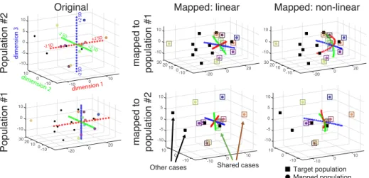
Fig. 2: Low-dimensional coordinates before and after domain adaptation. Dots corre-spond to the samples that are mapped to the target population, whose samples are represented by squares. Colored dots and squares stand for the 11 cases shared between the two populations: after mapping the colored dots lay near the center of the colored squares. The black dots and squares correspond to the remaining cases that also served to obtain the low-dimensional embedding, but were not used in the domain adaptation process. The red-green-blue curves represent the main directions of variation in the original population (from -2 SD to +2 SD), before and after mapping. Top: population #2 mapped to population #1, using the linear (middle) or non-linear right mapping. Bottom: similar plots for population #1 mapped to population #2.

atlas for population #2), different biomechanical models and therefore different modeling errors, and different personalization strategies —and potential errors in the personalization.

3.2 Parameters setting

We used 5 neighbors to construct the neighborhood graph of the Isomap dimen-sionality reduction algorithm. This value was chosen to minimize the relative im-portance of the second eigenvalue and the sum of eigenvalues (the compactness of the representation, illustrated in the right part of Fig.1), within a reasonable amount of possible neighbors (up to half the database).

The maximum amount of dimensions for the low-dimensional space was set to 14 (one unit less than than the size of the smallest studied population — population #2). Although the intrinsic dimensionality of the data may be lower (right part of Fig.1), some artifacts were observed in our implementation of the linear mapping when computing the scalar product (Ψ1)tΨ2 with cut

dimen-sions, which deserves further investigation.

Leave-one-out cross correlation was used to determine the regression param-eters (the weight γ and the bandwidth at which to stop the multi-scale scheme, determined as a fraction α of the samples density). The retained values were γ = 10 and α = 0.5, respectively.

(7)

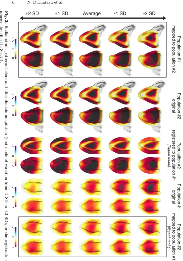
6 N. Duchateau et al. +2 SD +1 SD Average -1 SD -2 SD -0.5 0.5 0 -0.5 0.5 0 -2 2 0 -2 2 0 -2 2 0 Population #2 original Population #1 original Population #2 mapped to population #1 [flipped mod e] Population #1 mapped to population #2 Population #2 registered to population #1 [flipped mod e] Fig. 3: Radial strain patterns b efore and after domain adaptation (first mo de of v ariation from -2 SD to +2 SD), or the registration pro ce ss describ ed in Sec.2.1.

(8)

0 10

Non-linear Linear Non-linear Linear

-2SD -1SD 0 +1SD +2SD -2SD -1SD 0 +1SD +2SD -2SD -1SD 0 +1SD +2SD -2SD -1SD 0 +1SD +2SD 1 2 ... 14 dimensions

Fig. 4: Differences between the original deformation patterns and the deformation patterns reconstructed from the low-dimensional coordinates after domain adaptation, across all the modes of variation (Euclidean distance on the radial-circumferential-longitudinal deformation patterns treated as column vectors —as in Fig.1).

3.3 Transported coordinates

As observed in Fig.2, the cases that are shared between the two populations and that are used to compute the mapping were exactly matched (linear mapping) or almost exactly matched (non-linear mapping) in the target population space. The main modes of variation substantially changed after the mapping (a given mode in the original population is expressed as a combination of several modes of the target population after mapping).

We also observed the limits of the linear mapping, through substantial shrink-age of the variations around zero, due to the non-guaranteed correlation between the coordinates of the shared cases in the two populations, and therefore the po-tentially opposing contribution of some cases to the mapping. This shrinkage effect is still present for the non-linear mapping, but much less pronounced. Besides, the curvature of the modes of variation after the non-linear mapping supports the relevance of this mapping strategy against the linear one.

3.4 Domain-adapted patterns

Figure 3 illustrates the deformation patterns encoded in the first mode of varia-tions, before and after the domain adaptation. Patterns were reconstructed from low-dimensional coordinates evolving from -2SD to +2SD along the first dimen-sion. Reconstruction was achieved through the multi-scale regression presented above, with γ = 1 and α = 0.5.

As visible in Fig.3, the deformation patterns from populations #1 and #2 before domain adaptation substantially differ in terms of amplitude of the defor-mation, and spatial distribution of the patterns. This is even more visible when the patterns in the original population are transported to the target population by registration (as described in Sec.2.1). After domain adaptation, the mapped patterns are much closer from the target population both regarding amplitude and spatial distribution of the patterns. Subtle differences remain, which should correspond to the intrinsic differences between these two populations.

(9)

Figure 4 complements this information by quantifying differences between the original deformation patterns and the deformation patterns after domain adaptation, across all the modes of variation. With the linear mapping, patterns near the average are unchanged, due to the definition of this mapping (linear change of basis, centered around the average). Differences are not guaranteed to be concentrated on the first dimensions, as visible for dimensions 10 and 13. With the non-linear mapping, patterns near the average are also transported and therefore exhibit differences. Also, the modes of variation become curved (Fig.2) after domain adaptation, and differences between patterns are therefore not guaranteed to be symmetric on each side of the average.

4 Conclusion

We have demonstrated the potential of domain adaptation to compare databases from distinct sources, upon the constraint that some cases are shared between the databases to define the mappings. In our tested populations, non-linear mapping stands as a relevant solution, given that the distribution of the shared cases is not guaranteed to be the same across the two populations.

In terms of application, the approach is promising to better understand dif-ferences between populations from different sources (here, from different biome-chanical models), and may pave the ground for enriching a real database with simulated data or the comparison of different clinical cohorts. These perspec-tives will require further exploring up to which limit two different databases are actually compatible, and scaling the proposed methods to larger populations —including a substantial amount of cases shared between the two populations.

Acknowledgements. GK Rumindo was supported by the European Commission H2020 Marie Sklodowska-Curie Training Network (VPH-CaSE-642612). The authors also ac-knowledge the partial support from the French ANR (LABEX PRIMES of Universit´e de Lyon 11-LABX-0063], within the program “Investissements d’Avenir” [ANR-11-IDEX-0007]). Finally, the authors thank M Sermesant (INRIA Sophia-Antipolis, France) and J Ohayon (TIMC-IMAG Grenoble, France), who contributed to the de-velopment of the cardiac simulations, as well as P Croisille and M Viallon (CREATIS, CHU Saint Etienne, France), who provided the 9 cases used in population #1.

References

1. T Heimann, P Mountney, M John, et al. Real-time ultrasound transducer localiza-tion in fluoroscopy images by transfer learning from synthetic training data. Med Image Anal, 18:1320–8, 2014.

2. N Duchateau, M Sermesant, H Delingette, et al. Model-based generation of large databases of cardiac images: synthesis of pathological cine MR sequences from real healthy cases. IEEE Trans Med Imaging, 37:755–66, 2018.

3. R Moll´ero, X Pennec, Delingette H, et al. Multifidelity-CMA: a multifidelity approach for efficient personalisation of 3D cardiac electromechanical models. Biomech Model Mechanobiol, 17:285–300, 2018.

(10)

4. VY Wang, HI Lam, DB Ennis, et al. Modelling passive diastolic mechanics with quantitative MRI of cardiac structure and function. Med Image Anal, 13:773–84, 2009.

5. R Chabiniok, P Moireau, PF Lesault, et al. Estimation of tissue contractility from cardiac cine-mri using a biomechanical heart model. Biomech Model Mechanobiol, 11:609–30, 2012.

6. G Csurka. Domain adaptation in computer vision applications. Springer, 2017. 7. M Wang and W Deng. Deep visual domain adaptation: a survey. Neurocomputing,

312:135–53, 2018.

8. P Medrano-Gracia, BR Cowan, DA Bluemke, et al. Atlas-based analysis of cardiac shape and function: correction of regional shape bias due to imaging protocol for population studies. J Cardiovasc Magn Reson, 15:80, 2013.

9. S Sanchez-Martinez, N Duchateau, T Erdei, et al. Characterization of myocardial motion patterns by unsupervised multiple kernel learning. Med Image Anal, 35:70– 82, 2017.

10. E Puyol-Ant´on, M Sinclair, B Gerber, et al. A multimodal spatiotemporal cardiac motion atlas from MR and ultrasound data. Med Image Anal, 40:96–110, 2017. 11. RR Coifman and MJ Hirn. Diffusion maps for changing data. Appl Comp Harm

Anal, 36:79–107, 2014.

12. C Tobon-Gomez, M De Craene, K McLeod, et al. Benchmarking framework for myocardial tracking and deformation algorithms: an open access database. Med Image Anal, 17:632–48, 2013.

13. GK Rumindo, N Duchateau, P Croisille, et al. Strabased parameters for in-farct localization: evaluation via a learning algorithm on a synthetic database of pathological hearts. FIMH, LNCS, 10263:106–14, 2017.

14. A Bˆone, M Louis, B Martin, et al. Deformetrica 4: an open-source software for statistical shape analysis. ShapeMI, MICCAI workshop, LNCS, 11167:3–13, 2018. 15. J Tenenbaum, V De Silva, and J Langford. A global geometric framework for

nonlinear dimensionality reduction. Science, 290:2319–23, 2000.

16. A Bermanis, A Averbuch, and RR Coifman. Multiscale data sampling and function extension. Appl Comp Harm Anal, 34:15–29, 2013.