Control law designs for active suspensions in automotive vehicles

FOR

ACTIVE SUSPENSIONS IN AUTOMOTIVE VEHICLES

by

Chinny Yue

S.B., Massachusetts Institute of Technology

(1987)

Submitted to the Department of Mechanical Engineering

in Partial Fulfillment of the Requirements for the Degree of

MASTER OF SCIENCE IN MECHANICAL ENGINEERING

at the

MASSACHUSETTS INSTITUTE OF TECHNOLOGY

February 1988

( Chinny Yue, 1988

The author hereby grants to M.I.T. permission to reproduce and to distribute copies of this thesis document in whole or in part.

Signature of Author ijepq( ment of A A Mechanical Engineering January 15, 1988 Certified by

-3~<*

Chairman, Mechanical Engineering MASSACHUISET S INSTITUTJE

OF TIPiNOLOGY

MAR

18 1988

Professor A. A. Sonin Department Committee

ACTIVE SUSPENSIONS IN AUTOMOTIVE VEHICLES

by Chinny Yue

Submitted to the Department of Mechanical Engineering on January, 15, 1988 in partial fulfillment of the requirements for the Degree of Master of Science in

Mechanical Engineering

ABSTRACT

This study investigates the behavior of active suspensions designed with various control techniques for both a two-mass quarter-car model and a seven d.o.f. full-car model. The Linear Quadratic Regulator (LQR) and the Linear Quadratic Gaussian (LQG) compensator are used to improve the frequency response of the quarter-car model. Body isolation is improved at the sprung mass frequency in all designs, at the expense of increased suspension deflection at low frequencies and deteriorated axle response at the unsprung mass frequency. The LQG compensator with suspension deflection feedback, combined with semi-active control, gives the most satisfactory result : isolation is improved at most frequencies, with suspension and tire deflections maintained below the passive response at all frequencies.

Root mean square response of the full-car model subjected to random road inputs is studied at a speed of 80 km/hr, with time delay between the front and rear axles. A pole-placement method which can place the poles of heave and pitch modes indepen-dently, is developed by decoupling the heave-pitch modes. Driver's acceleration can be reduced by 45% without increasing suspension deflection, by choosing high damping and natural frequencies in the suspension and body heave modes. Application of the LQR by varying the penalties on the outputs shows that driver's acceleration can be reduced as desired and suspension deflection is reduced to a minimum of 57%. Tire deflection cannot be improved satisfactorily in either method. It was concluded that the LQR is a better approach in applications where output specifications are present.

Thesis Supervisor : J. Karl Hedrick

I would like to thank Professor Hedrick for his enthusiasm in this thesis, his con-tinuous guidance and advices, and his patience with me. I most admire his energy and his spirit of asking a lot of questions to get to the root of a problem. Discussions with him has often left me in an overwhelmed state of mind with questions and ideas enlightened by him.

I have had a great time in the Vehicle Dynamics Laboratory. A lot of thanks go to Dave Warburton who has been very helpful, especially in using use TEX which makes this thesis presentable. Then there are Jahng Park and Bill Stobart, my friendly company in front of the computer terminals; and of course the incredible Keith Laby and Behzad Rasolee, who provided great entertainments and fun times in the lab.

Almost everyone in the lab has helped me in one way or the other in the course of preparing this thesis. I would also like to thank Eduardo Misawa, John Moskwa, and Cathy Wong for helping me with the laser printing; and Ruth Shyu, Dave, and John for proof-reading this thesis.

Finally, I would like to dedicate this work to my parents who made my graduate study in M.I.T. possible; to my sister, Acme, and all my friends who care about me; and to my husband who is always there to give me the encouragement and motivation to finish this thesis in such a short period of time.

Chinny Yue began her college education in 1983 at Boston University as a computer science major. She transfered to the Department of Mechanical Engineering of M.I.T. in 1984 and was admitted to the Engineering Internship Program in 1985. She worked in Boston Edison Company in the summers of 1985 and 1986, where she also finished her bachelor's thesis on 'Reliability Analysis of the Reactor Core Isolation Cooling System of the Pilgrim Nuclear Power Station'. She began the research for this master's thesis in February 1987 in the M.I.T. Vehicle Dynamics Laboratory.

Chinny Yue is now working in the Network Services Planning Center of AT&T Bell Laboratories as a Member of Technical Staff.

Title Page . . . . Abstract . . . . Acknowledgements ... Biographical Note ... Table of Contents ... List of Figures . . . . Chapter 1 INTRODUCTION ....

1.1 The Automobile Suspension . . . 1.2 The Passive Suspension ...

1.3 The Active Suspension ... 1.4 Objective of this study ...

Chapter 2 QUARTER-CAR MODEL . 2.1 Model Description ...

2.2 The Passive Suspension ...

. . . . 10

. . . . 14

. . . . 17

. . . 20

. . . . 23

2.3 An Invariant Property of the Active Suspension 2.4 Controller Designs ... 2.4.1 The LQR method ... 2.4.2 Sprung Mass Velocity Feedback . . . . . 2.5 Compensator Designs . . . . 2.5.1 The LQG Compensator ... 2.5.2 Results . . . . 2.6 Comparison of Control Designs . . . . 2.7 Power Consideration for Semi-Active Control Chapter 3 FULL-CAR MODEL ... 3.1 Vehicle Model ... 3.1.1 Equations of motion ... 3.1.2 Output equations ... 3.2 Disturbance model ... 3.2.1 Model Description ... 3.2.2 Covariance Propagation Equation . . .. 3.3 Power Consumption ... S . . . . . 29 . . . . 31 . . . . 31 S . . . . . 38 S . . . . . 46 . . . . 46 . . . . 49 S . . . . . . . 57 . . . . . 59 . . . . 68 . . . . 68 . . . . 71 . . . . 73 . . . . 78 . . . . 78 S . . . . . 82 . . . . 86

4.1 Decoupling and Pole-Placement . . . . . 4.1.1 Methodology ...

4.1.2 Physical Interpretation of Body and Susjpension 4.1.3 Pole-Placement Results . . . . 4.2 Linear Quadratic Regulator . . . .

4.2.1 Problem Definition ...

4.2.2 Improvement of Isolation . . . . 4.2.3 Improvement of Suspension Deflection . . . 4.2.4 Improvement of Tire Deflection . . . . 4.3 Discussion of the Two Methods . . . . Chapter 5 CONCLUSION AND RECOMMENDATION References . . . . Appendix A EQUATIONS OF MOTION . . . .

A.1 System Equations ... A.2 Output Equations ...

Appendix B POLE-PLACEMENT PROCEDURES .

. . . . . . 88 . . . . 88 Modes . ... 92 . . . . . 94 . . . . .109 . . . .109 . . . . .110 . . . . .115 . . . . .118 . . . . .119 S . . . 121 . . . .124 S . . . . .128 . . . .128 . . . .133 . . . . .134

Figure Figure Figure Figure Figure Figure Figure Figure Figure Figure Figure Figure Figure Figure Figure Figure Figure Figure Figure Figure Figure Figure Figure Figure Figure Figure Figure Figure 1.1 1.2 1.3 2.1 2.2 2.3 2.4 2.5 2.6 2.7 2.8 2.9 2.10 2.11 2.12 2.13 2.14 2.15 2.16 2.17 2.18 2.19 2.20 2.21 2.22 2.23 2.24 2.25

Figure 2.26 _{Semi-active control in LQG design measuring sd . . . . . 66} Two d.o.f. suspension model . . . .

Effect of damping in a passive suspension [2] . . . Relationship between various vehicle outputs [2] . . Quarter-car model and vehicle parameters . . . . Block diagram of the quarter-car model . . . . . Body acceleration in passive suspension . . . . . Suspension deflection in passive suspension . . . .

Tire deflection in passive suspension . . . . Block diagram of LQR loop . . . . Root locus of LQR ...

Body acceleration in LQR design . . . . Suspension deflection in LQR design . . . . Tire deflection in LQR design . . . . LQR design without amplification in wheel-hop mode Body acceleration in LQR design with g3 = 0 . . .

Root locus of sprung mass velocity feedback . . .

Body acceleration in sprung mass velocity feedback . . . Suspension deflection in sprung mass velocity feedback . . Tire deflection in sprung mass velocity feedback . . . . . The LQG compensator ...

Body acceleration in LQG design with velocity feedback Suspension deflection in LQG design with velocity feedback Tire deflection in LQG design with velocity feedback . . . Body acceleration in LQG design measuring d . . . . . Suspension deflection in LQG design measuring sd . . .. Tire deflection in LQG design measuring sd . . . .

Semi-active control in the LQR design . . . . Semi-active control in absolute velocity feedback . . . . .

10 12 . . . 13 . . . 21 . . . 21 . . . 25 . . . 26 . . . 28 32 34 35 37 . . . 39 . . . 40 . . . 41 . . . 42 . . . 43 44 45 S.. .47 . . . 51 . . . 52 . . . 53 . . . 54 55 56 . . . 62 . . . 64

Figure Figure Figure Figure Figure Figure Figure Figure Figure Figure Figure Figure Figure Figure Figure Figure Figure Figure Figure Figure Figure 3.2 3.3 3.4 3.5 3.6 4.1 4.2 4.3 4.4 4.5 4.6 4.7 4.8 4.9 4.10 4.11 4.12 4.13 4.14 4.15

Parameters of vehicle with passive suspension [16]

Natural frequency w, and damping ratio ý of vehicle modes Power spectral density of road input at each corner . . . R.M.S. acceleration at driver's seat at different velocities . Root mean square values of outputs at 80 km/hr . . . . a. Passive suspension model . . . . b. Active suspension model

Driver's acceleration in suspension heave pole-placement Suspension deflections in suspension heave pole-placement Front tire deflections in suspension heave pole-placement Rear tire deflections in suspension heave pole-placement Power consumption in suspension heave pole-placement

. . . . . . 102 . . . . . .103 . . . . . .104 . . . . . .106 method . 107 . . . . . .112 . . . . . .113 ... .... 114

Improvement of average suspension deflection by the LQR LQR design at point A ... . . 116 S. 117 76 * . . 77 * . . 81 * . . 84 * . . 85 * . . 93 * . . 96 * . . 97 * . . 98 . . . 99 . . . 101

Driver's acceleration in body heave pole-placement Suspension deflections in body heave pole-placement Tire deflections in body heave pole-placement . . . Power consumption in body heave pole-placement . a. Vehicle outputs of three designs by pole-placement b. Control gain of the best design

Improvement of driver's isolation by the LQR . . . Vertical acceleration of the c.g. in the LQR . . . .

LQR design at pi = 140 ...

1.1

The Automobile Suspension

The automobile suspension is the system of devices which supports the vehicle body on the axles. The vehicle body refers to the sprung mass, which consists of the housing as well as its contents, the engine, and other mechanical parts. The axles refer

to the unsprung masses, which consist of the wheels and tires, the wheel hubs, the brake discs, and part of the drive shafts and steering linkages that are not supported by the suspensions and thus not considered as sprung masses. The suspension system may consist of springs, dampers and actuators.

The suspension performs two functions, namely ride quality and handling. To provide good ride quality, the suspension should support and isolate the sprung mass

from external disturbances, such as road irregularities which account for most of the discomfort perceived by passengers. In general, ride quality can be measured by the vertical acceleration of the passenger; roll and pitch were found not to play a significant role in ride quality [1]. The standard for ride quality is subjective. Where one may prefer a well-isolated soft suspension, another may desire a stiffer ride, since it provides a greater feeling of the road surfaces and thus more control.

Vehicle handling is a measure of the vehicle performance as well as the "feel" it conveys to the driver during maneuvers of acceleration, braking or cornering. The "feel" means the feedback received by the driver through the steering wheel, brake pedal, and more. Therefore, handling is a term too subjective to be quantified. For this study, the aspect of handling that is of interest is roadholding, which is the ability of the suspension system to control the motion of the unsprung masses so as to maintain the tires in firm contact with the road despite any road disturbances. This is necessary because the contact force at the tire-road interface generates the traction needed for acceleration and braking, and the lateral tire forces needed for cornering. Therefore, a good suspension should reduce as much as possible any variations in the tire force, or equivalently, the tire defieciton, resulting from road irregularities.

Figure 1.1 Two d.o.f. suspension model

1.2

The Passive Suspension

Studies [1,21 on the performance characteristics of the passive suspension have been done using the car model shown in fig. 1.1. This is a linear two degree-of-freedom

(d.o.f.), lumped element model, with motion in the vertical direction only. The sus-pension is simply modeled by a spring and damper. This simple ride model was used to gain fundamental qualitative understanding of the limitations to the performance of passive suspensions.

The results from [2] are shown in figs. 1.2 and 1.3. There are two natural modes of vibration of the suspension system, typically one at 1 Hz associated with the sprung mass, and the second one at about 10 Hz associated with the unsprung mass. Fig. 1.2a shows the sprung mass acceleration per unit velocity input over the frequency spectrum, for three damping coefficients. It can be seen that high suspension damping improves the isolation of the sprung mass at low frequencies, worsens it up to the second resonance peak, and beyond that, the roll-off rate is deteriorated. The frequency plot in fig. 1.2b illustrates the effect of damping on tire deflection. Low damping results in pronounced peaks at the two natural frequencies but reduced tire deflection at the in-between frequencies. As more suspension damping is applied, the peaks at the natural frequencies are reduced. However, this is accompanied by increased tire defleciton in

the mid-range frequencies. Malek [1] obtained similar results and conclusions for the compromises in selecting the suspension damping.

The plot in fig. 1.3 shows the normalized dimensionless root mean square (r.m.s.) values of the sprung mass acceleration versus the suspension deflection, along with contour plots of constant levels of tire deflection. As damping is increased, both r.m.s. acceleration and r.m.s. suspension deflection are decreased, until at a certain point, the trend is reversed and the r.m.s. vertical acceleration begins to increase. The same applies to tire deflection. As damping is increased, r.m.s. tire deflection decreases at first and then increases again.

The effect of suspension stiffness can also be examined by comparing the different curves. When the stiffness is decreased (stiffness ratio increased), the curve is shifted down, indicating an improvment in vibration isolation. However, a soft suspension results in large suspension stroke. This trade-off has also been demonstrated in [3] using a one d.o.f. model. For all practical purposes, the stiffness ratio cannot be

increased beyond 20.

A basic trade-off in the performance of passive suspension exists, where a soft suspension reduces the effects of road disturbances on body vibration, with increased suspension clearance; a hard suspension reduces the effects of external forces such as gravity, aerodynamic forces and centrifugal forces, resulting in reduced suspension stroke but increased body vibration. The presence of both road disturbances and exter-nal forces, and the passenger isolation versus suspension excursion requirement, results in competing factors in suspension design. In addition, as body isolation is improved, the axle response can get worse and the road-to-wheel contact is deteriorated [4]. Other performance limitations of passive suspensions include lateral acceleration experienced during cornering which causes excessive roll-out of the body, and longitudinal acceler-ation or deceleracceler-ation which produces excessive lifting or diving.

Although there exists in current car productions electronically adjustable suspen-sion springs and dampers so that the designer or the driver can adjust the parameters as desired to suit one's driving taste, the biggest problem one faces remains to choose the optimal spring stiffness and damping. There are two reasons for the basic limi-tations of passive suspensions : a) there is no external power requirement, thus the suspension can only store or dissipate energy ; b) the suspension can only generate forces in response to local relative motion.

0.1

0.01

10 100

Frequency (rad/s)

a. Vertical acceleration response

10 100

Frequency (rad/s)

Figure 1.2

b. Tire deflection response

Effect of damping in a passive suspension [2] 1000 E E o 0 001 0 0001 1000

1.0 2.0 3.0 4.0 5.0 6.0 7.0 8.0 9.0 10.0 RMS Suspension Travel

[7ý0U

Figure 1.3 _{Relationship between various vehicle outputs [2]}

LO C-U) 0 0o tC₀ 0 O C. 0..) <: .-_ rco₀ 0 U U) or' 0.28 0.24 0.20 0.16 0.12 0.08 0.04 0.00 11.0 12.0

1.3

The Active Suspension

The passive suspension suffers performance limitations due to the constitutive rela-tions imposed by the spring and the damper. The suspension can only dissipate energy stored in the springs and dampers, and the suspension force can only be functions of relative displacement and relative velocity of the suspension. In order to circumvent these shortcomings of conventional suspensions, active suspensions were proposed. By adding to the suspension an active force actuator, which may be hydraulic, pneumatic, or electric, the force input to the active suspension can be modulated according to any arbitrary control law. Variables, such as driver's acceleration or suspension travel, can be measured by sensors and analysed by an onboard computer in which the control law has been implemented. Electronic signals from the computer then command the amount of force delivered by the actuator. Thus, the suspension force can be a function of any variable, either local or remote, relative or absolute. Since energy is continually supplied to the active suspension, the force generated does not depend upon energy previously stored in the suspension. The spring and damper should still be retained parallel with the actuator in case the actuator suffers a power failure.

The active suspension has the ability to simultaneously appear soft for body iso-lation and hard for external forces and small suspension travel; whereas a passive suspension with fixed properties, provides only a compromise between a hard-and-soft suspension. Active suspensions are able to provide better passenger isolation, or equiva-lent isolation while operating at higher speeds or over rougher roads than a comparable passive suspension. The disadvantages of active suspensions are the increased cost and complexity due to the need for an external power source, and the reduced reliability.

Active suspension has been under research and development since the 1930's. Re-views by Hedrick and Wormley [3], and by Goodall and Kortiim [5], summarize studies in active suspensions for ground transport vehicles and control techniques for the de-sign and optimization of active suspensions. These control strategies include parameter optimization [6], frequency domain [7,8], and state-space [9,10,11] techniques.

There have been numerous papers devoted to active suspension designs using sim-plified models. Paul and Bender [12] have derived an active suspension for a two d.o.f. model using both sprung and unsprung mass acceleration and velocity feedback, with a passive spring and damper between the two masses to achieve optimum performance. Karnopp [13] has applied absolute damping to body velocity in a two d.o.f. model, to

improve body isolation as well as wheel resonance by suitably choosing the mass ratio. Active damping was also incorporated with a high-gain load leveler for static loads such as the vehicle weight. A two d.o.f. heave-pitch model has been used in [14] to investigate the frequency response to heave and pitch inputs by employing fully-active and semi-active suspensions, using state variable feedback and absolute velocity feed-back. The results show that the active systems are far superior to conventional passive suspensions.

Malek [1,15] has used active suspension to decouple the heave and pitch modes of a full-car model, combined with absolute velocity damping. Body pitch transmissibil-ity to heave input (and vice versa) was reduced. Fore-aft tire load transfer was also reduced, which improved roadholding characteristics. Chalasani [2,16] has studied the ride performance of active suspensions by applying a full-state, optimal linear regula-tor to both a quarter-car model and a full-car model. It was shown that the active suspension is superior to the passive one for random, discrete, and periodic road inputs. Besides linear, state-space methods, there is a wide spectrum of techniques in the frenqency domain as well as non-linear methods. A method proposed by Thompson [4] simultaneously improves ride quality and increases overall stiffness to resist external forces, and can be used in series and parallel arrangement of control elements. When a series arrangement of dynamic dampers is used to control axle vibrations, isolation at the wheel-hop frequency can be reduced by using a parallel feedforward compensa-tion circuit. Kimbrough [17] has modeled variable component suspensions as bilinear systems and applied nonlinear regulators. The suspension design produces significant improvements in ride quality without severely deteriorating roadholding or violating packaging requirements. Bender [18] has used a look-ahead sensor to obtain preview information in a one d.o.f. system and reduced both body acceleration and suspension deflection. An optimum linear suspension has been derived in [19] which minimizes heave acceleration subject to a constraint in suspension deflection, and can be applied to the active control of a flexible-skirted air cushion suspension, which couples a vehicle model to a guideway having random irregularities.

In recent years, numerous car companies have shown interest in active suspen-sion research. Lotus Car Ltd. built a prototype with fully active computer-controlled suspension which reads road surface and driver-command inputs and self-adjusts hy-draulically to accomodate them. In a test drive report [20] of the prototype, it was

shown that the active suspension is able to maintain a stable and level ride condition on rough and bumpy roads which normally would shake the driver in a passive suspension. The nose does not lift (or dive) during acceleration (or braking). It corners absolutely flat and can even roll inward if required. The hydraulic actuators react so rapidly under computer control that only 70 percent of the suspension travel is used compared to the passive suspension at the same speed on the same road conditions. This means the active car can actually traverse 30 percent faster to reach the same limit in the passive one. Moog variable-flow servo valves are the interface between electronics and hydraulics and are capable of turning small electronic commands from the computer into powerful hydraulic actions.

The benefits of active suspensions are far-reaching. There would be no need to install a wide range of different suspensions, springs, dampers and anti-roll bars. All it needs is a common actuator system, with a different program chip for different car models (eg. luxury or sporty cars). All the hardware can be common; only the software needs to be changed. Since active control provides better roadholding capabilities, which means making better use of the tire-road contact area, higher performance may be obtained from narrower tires. Narrower treads that reduce rolling resistance and thus enhance fuel economy may be exploited. Also, the smaller suspension movement resulting from active control means wheel arches can be tighter or fender lines lower. This provides entirely new freedom in chassis styling.

1.4

Objective of this study

The variables of concern in this study are : a) ride quality, the capability of the suspension to isolate the vehicle body from vibrations, measured by the sprung mass acceleration (for quarter-car model) or the vertical acceleration at the driver's seat (for full-car model); b) suspension packaging and clearance requirement which is directly affected by suspension deflection; c) roadholding capabilities, measured by the tire force or tire deflection; and d) the mechanical power required by the actuators so that external power requirements and actuator size may be determined.

In the first part of this study, Chapter Two, the two-mass heave-only quarter-car model in fig. 1.1 is used to investigate different control techniques and the improvement in the frequency response of the outputs due to road disturbances. The techniques are : the Linear Quadratic Regulator (LQR) and absolute velocity feedback for controller designs, and the Linear Quadratic Guassian (LQG) for compensator designs.

The LQR requires full-state feedback and perfect measurement. Cost or penalties are imposed on the various outputs and controls, and the optimal control gain is the one which results in minimum cost. The second technique is to feed back sprung mass velocity measurement through a constant gain, which is equivalent to output feedback in classical control. The LQG compensator requires measurement of only one output and uses a Kalman Filter to reconstruct the states. Suspension deflection and sprung mass velocity are used for output feedback in this study. The Loop Transfer Recovery (LTR) method, traditionally used in tracking problem, is also briefly discussed.

These control designs will be compared in terms of the frequency response of body isolation, suspension deflection and tire deflection. The application of semi-active control, which requires little external power, to approach the fully-active designs will also be discussed.

In the second part of this thesis, the seven d.o.f. full-car model developed by Malek [1] is used. There are three modes of vibration in the sprung mass : heave, pitch, and roll; and four modes in the unsprung masses : heave, pitch, roll, and warp. The choice of state variables is suited to reflect the coupling between heave and pitch, and between roll and warp.

Malek decoupled the heave and pitch modes and introduced absolute damping (absolute velocity feedback) in designing the active suspension. By ad hoc selection,

the decoupled configuration was obtained by simply setting all coupling terms to zero, and the absolute damping was forced to duplicate the relative damping. In other words, only one special case was studied and it was assumed that this was the closed-loop configuration desired. The analysis did not provide general guidelines to reach the closed-loop system matrix given certain desired features of the active suspension, eg. pole locations in the heave mode resulting in a soft or stiff ride. The design freedom in choosing the absolute damping terms and other decoupled configurations were not investigated. Thus, the question remains to decide how to decouple the system and how much absolute damping should be used, so that the final active system has certain desired characteristics.

As already mentioned, Chalasani [16] designed the active control law by applying the optimal Linear Quadratic Regulator (LQR) to a similar full car model. A cost function was defined by ad hoc selection of the penalties on the controls and various outputs. Although the study showed that the suspension system was improved, the power consumption in the active control was not evaluated. The power requirement in the actuators might be too high to be physically or economically realizable. Note that the control design is optimal only with respect to the cost function so chosen. The analysis did not investigate the design freedom in defining the cost function which directly affects the trade-offs between the power requirement and the improvement in the suspension system.

The objective of this study is to apply the decoupling and the LQR methods to design the active suspension system for a vehicle traveling in a straight line at constant speed subjected to random road disturbances. The sinusoidal road input used by Malek is useful for understanding the coupling effect between the modes, but it does not represent a realistic road. Thus, the road disturbances at the four wheels are modeled as stochastic inputs through first-order filters, with a time delay between the front and rear wheels. The covariance propagation equation is modified to take the time delay into account. The outputs and power requirement will be evaluated in terms of their r.m.s. values.

A decoupling and pole-placement methodology is developed in this study to first decouple the heave and pitch modes of the vehicle, and then to use absolute feedback, the active portion of the control, to arbitrarily place the poles of the decoupled modes. Absolute feedback includes both absolute velocity and absolute displacement feedback.

Notice that in a pure decoupling strategy, no active control is needed to decouple the system. The r.m.s. response of the vehicle and the power requirement are investigated for poles of different natural frequencies and damping coefficients.

In the LQR approach, the penalties on the control force and outputs are varied in different ways to obtain different cost functions, in order to study how much im-provement one can get in an output, given the amount of power available, without deteriorating the other two outputs.

Chapter Three summarizes the full-car model in state-space form and identifies the important parameters. Stochastic road disturbance model and the covariance propa-gation calculation are then discussed. Some r.m.s. results of the passive system are presented for comparison in later chapters.

Chapter Four presents the two control strategies to design the active suspension. In the first part, the decoupling-pole-placement methodology is developed. The signifi-cants of the poles of the sprung mass and suspension are given physical interpretation. The results provide some general guidelines in choosing the appropriate pole locations of the decoupled modes. In the second part, the LQR method is applied and the cost function adjusted to obtain the relationship between power consumption in the actuator and improvements (reduction) in the r.m.s. values of the driver's vertical acceleration, suspension deflection, and tire force.

QUARTER-CAR MODEL

2.1

Model Description

A two-mass, quarter-car model is used in this chapter to study vehicle response to road disturbances by using control techniques which include controller designs by the Linear Quadratic Regulator (LQR) and absolute velocity feedback, and compensator designs by the Linear Quadratic Gaussian (LQG) method.

The model is shown in fig. 2.1 along with the numerical values of the car parameters obtained from [2]. The suspension is modeled as a linear spring of stiffness k, and a linear damper of damping coefficient b,. The tire is simply modeled by a spring of stiffness kt. The actuator force u is positive whenever the suspension is compressed.

The state variables are chosen to be :

Xl = z, - z, suspension deflection X2 = i8 sprung mass velocity

X3 = zu - zo tire deflection

X4 = zu unsprung mass velocity

The system equations can be represented in state-space form :

x = Ax + Bu

+

m, = 240 kg mu = 36 kg

b, = 980 N-sec/m

k, = 16,000 N/m kt = 160,000 N/m

Figure 2.1 Quarter-car model and vehicle parameters

Figure 2.2 Block diagram of the quarter-car model

A block diagram of the system is shown in fig. 2.2. This simple model is used to gain fundamental insights into the suspension control problem without greatly complicating the analysis.

The output of primary concern is the acceleration of the sprung mass, as, which is a measure of vibration isolation.

as = Clx+ dlu (2.2)

where C1= [k _m _bL_ 0 _bI_ ], dl = l/m,

8, m, m

The other outputs that need to be examined the tire deflection td, expressed as follows :

sd = C2x

are the suspension deflection sd and

(2.3)

whereC _{2 = [1 0 0 0 ],0}

td = C3x (2.4)

where C3= [0 0 1 0].

Combining eqs. 2.2 to 2.4, the output vector y which represents as, sd and td can be expressed in state-space form :

2.2

The Passive Suspension

This section investigates the properties of the passive suspension by looking at the locations of system poles and zeros, and the response of the vehicle outputs to road disturbances.

The system characteristic polynomial is :

d(s) = mm ,s4 + (m, + m,)b,s3 + ((m+m, + m)k. + m, kt)s2 + b.kts + k.kt (2.6)

There are two pairs of conjugate poles in the system from eq. 2.6 (i.e. eigenvalues of matrix A) :

sprung mass mode w, = 1.25 Hz S = 0.22 unsprung mass mode w, = 11 Hz I = 0.2

where w, is the natural frequency and ' is the damping ratio.

System zeros can be obtained by the transfer functions from the control input u to the outputs. The transfer function from u to as is :

C

(s)B + d

(

_{+ k)}

_(2.7)

d(s)

with zeros at 0, 0,

f±j

C2(s)B = + k (2.8)

d(s)

with zeros at

i±j--

2ms

C3b(s)B = d(s) (2.9)

with two zeros at 0. All of the zeros lie on the imaginary axis. Thus, the system is non-minimum phase with respect to the individual outputs. There are, however, no zeros corresponding to the transfer function CD(s)B, meaning that there is no frequency at which none of the three outputs are excited by the control force.

The primary concern of this chapter is the response of the vehicle outputs to road disturbances. Thus, Has(s) is defined as the transfer function from io to as :

Ha,(s) = C1((s)L

kts(bas _{+ k),)}

= d(2.10)

d(s)

The shape of Ha,(s) can be predicted by taking limits at low and high frequencies

lim Has(s) = s (2.11)

8--*0

lim Has(s) = k (2.12)

m9-00oo ums, S2

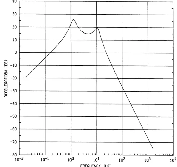
The gain increases at a slope of 20 db/dec at low frequencies and rolls off at -40 db/dec at high frequencies, as shown in fig. 2.3. The two peaks correspond to the two pairs of system poles.

The transfer function from disturbance io to suspension deflection sd, is defined

as

Hd(s)

:

H,d(s) = C24(s)L

ktmas

ktms _(2.13)

d(s)

The bode plot of Hd(S) has the property :

lim Hd(s) = -- s (2.14)

8--.0 k8

lim Hsd(S) = - _(2.15)

8--oo 00

The slope of Hed(s) at low frequencies is 20 db/dec and the gain rolls off at -60 db/dec at high frequencies as shown in fig. 2.4.

The transfer function, Htd(S), defined from io to tire deflection td, is :

Htd(s) = C3 (s)L

mms• _• + (m + + m9)b9s2 _{+ (mU + m,)ks}

(2.16) d(s)

10-1 100 101 102 103 FREQUENCY (HZ)

Figure 2.3 Body acceleration in passive suspension

40 30 20 10 0 O -10 z - -20 .J C -30 -40 -50 -60 -70 -80 10-2 104

10-1 100 101 102 103 FREQUENCY (HZ)

Figure 2.4 _{Suspension deflection in passive suspension}

0 -20 -40 -60 z U -80 _J U-_L, z -100 LU L-) _-120 U3 -140 -160 -180 10-2 104

The shape of Htd(S) can be predicted by : lim Htd(S) = -(m + m₈)s (2.17) S---0 Ikt 1 lim Htd(s) = (2.18) --- oo S

and is shown in fig. 2.5. The slope of the asymptote is 20 db/dec at low frequencies and -20 db/dec at high frequencies.

The system is observable from all three outputs and all the states are controllable. Control laws will be designed for the suspension system, to improve vehicle response due to road disturbances, particularly in the vicinity of the two resonance peaks.

10-1 100 101 102 103

FREQUENCY (HZ)

Figure 2.5 Tire deflection in passive suspension

-25 -30 -35 -40 -45 -50 -55 -60 -65 -70 -75 -80 10-2

2.3

An Invariant Property of the Active Suspension

The most general form of control law is :

u = -Gx _(2.19)

where G =[g g2 93 g94 ].

All states are perfectly measured in real time and used in feedback through the gains. g1 acts on the suspension deflection and primarily affects the frequency of the

sprung mass mode. g3 acts on tire deflection and affects the frequency of the wheel-hop mode. g2 acts on the absolute velocity of the sprung mass and provides damping for

the sprung mass mode. g4 acts on the unsprung mass velocity and affects the damping

of the wheel-hop mode. By using active control, the frequency and damping of the two modes can be set independently of each other, whereas in a passive suspension, these properties are affected by the same spring and shock absorber in the suspension.

All of the control techniques to be investigated in this study can be implemented by the control law in eq. 2.19. The LQR method uses full-state feedback, thus all the gains are non-zero. When absolute velocity feedback is used, all gains are zero except g2. In a dynamic compensator, estimated states X, instead of x, are used in feedback

and acted on by G.

There is an invariant property of the acceleration transfer function at the wheel-hop mode frequency which does not depend on the control laws. The equations of motion for the sprung and unsprung masses are :

mz, = control force + spring force + damper force (2.20)

m,i, = -control force - spring force - damper force + kt(zo - z,) (2.21)

The forces in the actuator, the spring, and the damper acting on the sprung and unsprung masses are equal and opposite. Adding the two equations :

ms z + mu z-

=

kt(zo

-

zU)

(2.22)

It can be shown from eq. 2.22 that the relationship between the acceleration and sus-pension deflection transfer functions is :

mus2 + kt kt

Has (s)

-

Ha(S)

+

which gives :

Has(s) =

at s

=

kt/mu

(2.23)

There is an invariant point in the acceleration transfer function at 10.6 Hz where the gain is always 20 db. It only depends on the masses and the tire stiffness, no matter what the suspension stiffness and damping are (see fig. 1.2a), and what kind of control law is implemented in the actuator.

2.4

Controller Designs

2.4.1 The LQR method

The LQR is a dynamic optimal controller which requires full-state feedback to minimize a quadratic cost function. The LQR technique has had major impact in modern control theory and practice, and many papers have been written on it. The LQR problem will be formulated and the solution summarized below [21,22,23].

Given the model of the vehicle :

i = AX + Bu

a quadratic cost function J is defined : 00oo

J = f(Q_ + u'R_)dt (2.24)

0

where Q is a state weighting matrix assumed symmetric and positive semi-definite. Q

must be expressed as N'N (i.e. Q=N'N). R is the control weighting matrix assumed symmetric and positive definite. Q and R represent the cost or penalties of state variables and controls. The trade-off can immediately be seen in J where expensive control (thus small u) drives the states to equilibrium slowly (large x); whereas driving the states very fast requires large and cheap control. The minimum of J is always positive.

A variant of the LQR problem is to include cross-coupled cost between states and controls :

o00

J = (_'Qx + 2x'Su + u'Ru)dt -(2.25)

0

with the requirement that :

Q S

be positive semi-definite. Matrix S represents the penalties on certain directions of the states and controls.

Figure 2.6 Block diagram of LQR loop

It is required that the pair [A,B] be stabilizable and the pair [A,N] be detectable. Then the optimal control problem is to find the control u that minimizes the cost function J subject to the constraints in the differential equations of the system. Solution of the LQR problem, i.e. the gain matrix G, exists and is unique. It is realizable in full-state feedback form as in eq. 2.19 , provided that all state variables can be measured in real time.

G = R-I(S' + B'K) (2.26)

where matrix K is the unique symmetric positive semi-definite solution of the control algebraic Riccati equation (CARE) :

-KA - A'K - Q + (KB + S)R-1(B'K + S') = 0

(2.27)

The CARE can be easily solved off-line by control design software, such as MATRIXx [24]. Fig. 2.6 shows the visualization of the LQR loop in block diagram.

An advantage of the LQR method is that the eigenvalues of the closed-loop system matrix [A-BG] are guaranteed to be in the left-half of the s-plane. Stability of the closed-loop system is assured no matter what the numerical values of A, B, Q, R and S are.

In a numerical problem, Q, R and S are the real-life costs of controls and states. In this study, they become design parameters that can be experimented with to obtain

the desired closed-loop properties. In a first step to define J, it is desired to equally penalize the three outputs, instead of the four state variables. The cost of the control is represented by a scalar parameter p. The cost function becomes :

oo

J = (y'(Iaxa)y + pu2)dt (2.28)

0

This can be rewritten as :

00 J =/('Q+ Ru2 + 2x'Su)dt (2.29) 0 where Q = c'C R = D'D + p S = C'D

It has already been shown that the plant is controllable and observable, thus the LQR requirement of stabilizability and detectability are satisfied. The LQR can be applied to solve for the gain G. The closed-loop system equations become :

i = (A - BG)_ + Lzo (2.30)

y = (C - DG)x (2.31)

The closed-loop characteristic polynomial is :

d(s) = m,,ms 4 _{+ ((b, + gs)mu + (b, - g4)m,)s}3

+((ka + gl)mu + (kt + k, + gi - g3)ms)s 2 + (b, + g2)kts + (k, + gl)kt (2.32)

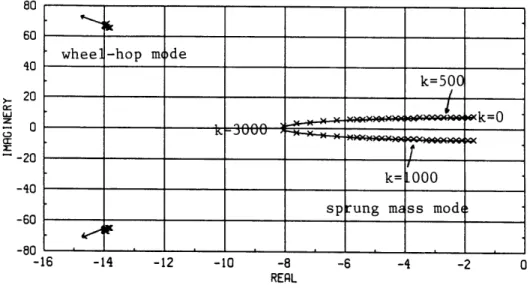
The root locus plot is shown in fig. 2.7 by computing the closed-loop pole locations for different values of p. As p is decreased, the poles of the sprung mass mode move away from the imaginary axis and become faster and more damped, whereas those of the wheel-hop mode move towards the imaginary axis and become slower and less

1-hop m( p =- 10-5 )de i-_ p = 10- 5 )rung ma

sI

Figure 2.7 Root locus of LQR

damped. The LQR method improves system response at the but reduces damping at the second peak.

first resonance frequency

The acceleration transfer function Ha,(s) is evaluated for the closed-loop system : , s(mng3s2 _{+ (b, - g4)kts + (k, + gl)kt)} H7aekS) = d(s) lim Ha,(s) = s 8--0 lim Hae(s) = (93 -oo00 ma (2.34) (2.35)

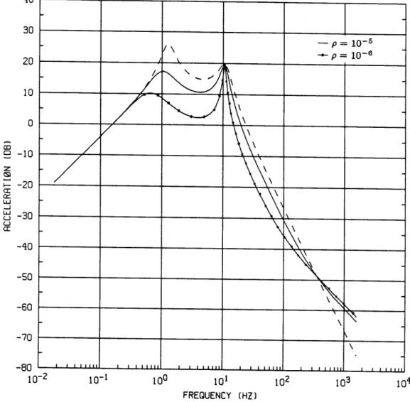
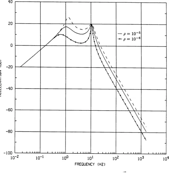
The gain at high frequencies rolls off at -20 db/dec, a smaller rate than that of the passive system because of the additional zero in eq. 2.33. This zero is due to the feedback gain g3 of the tire deflection. The low-frequency asymptote does not change. Fig. 2.8 compares the passive and active designs at two values of p. The passive response is shown as dashed lines in all the plots that follow. Isolation is improved at the first peak but unchanged at the second peak. The gain at 10.6 Hz is, as expected, invariant at 20 db, independent of changes in p. Isolation is deteriorated at high frequencies because of the additional zero.

p = 0.1 whee @4 -60 -Rn -14

=I

101

FREQUENCY (HZ)

Figure 2.8 _{Body acceleration in LQR design}

- p = 10-5 "-"- p = 10-6

/

/

The suspension deflection transfer function Hd(S) becomes :

H(93m,

-

(kt

-

93)m,)s

-

(g2

+

g4)kt

Hsd(S)=

(2.36)

mm,s

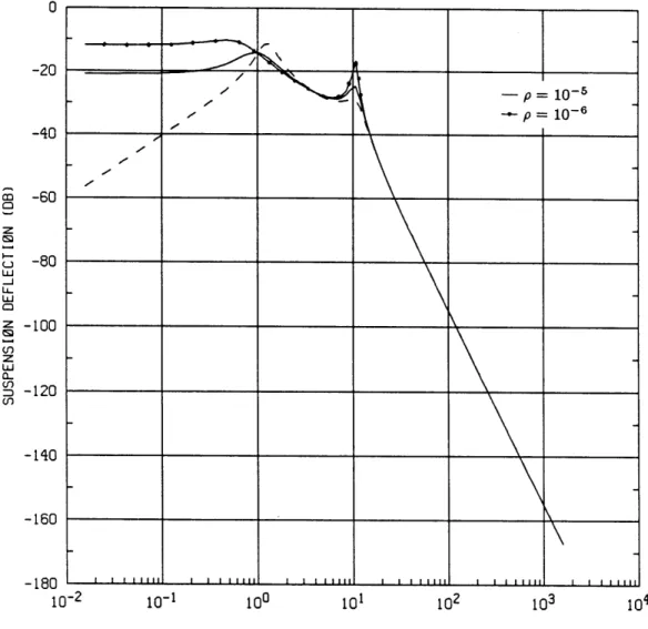
The high-frequency asymptote remains the same as that of the passive system. The zero in eq. 2.36 is at some non-zero frequency whereas the zero in eq. 2.13 (for the passive system) is at 0 Hz. This occurs because of the sprung and unsprung mass feedback gains, g2 and g4. The low-frequency gain stays constant at a non-zero value, which means suspension deflection is larger than that in the passive system. These predictions are verified by fig. 2.9. The disturbance is amplified in the suspension for frequencies up to the sprung mass mode. This can be explained by examining the physical situation at low frequencies. The disturbance zo can be treated as a constant velocity input. Since the tire is much stiffer than the suspension, and the imaginary absolute damper almost prevents the sprung mass from having any velocity, the suspension has to absorb most of the velocity input by going through more deflection. This deflection amplification gets larger as more control gains are used, as seen from eq. 2.37. There is a very slight improvement at the first peak, followed by an amplified peak at the second resonance frequency, due to the reduced damping of the poles of the wheel-hop mode as discussed before. The gain at high frequencies rolls off at the same rate as the passive response. The ability of the tire to follow the road is evaluated by the tire deflection transfer function Htd(s) : mm) s3 + ((6b - g4)m, + (b, + g2)m)u) 2 + (k. + g1)(mu + m,)s

Htd(S)

=

d(s)

(2.39)

10-1 100 101 102 103

Figure 2.9 _{Suspension deflection in LQR design}

0 -20

-40

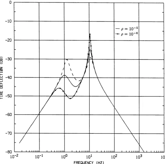
The bode plot of Htd(S) is shown in fig. 2.10. The first peak is reduced but the second peak amplified for the same reason discussed in suspension deflection. The high and low frequency asymptotes are identical to the passive system, independent of p.

More control is used as p is decreased or the penalty on as is increased. This results in more improvement in body acceleration at most frequencies and a sharper rise in the gain at the unsprung mass frequency to return to the invariant point. The tire deflection is also improved at the first peak. However, all of the above are accom-panied by increased suspension deflection at low frequencies, deteriorated isolation at high frequencies, and amplified suspension and tire deflection at the wheel-hop mode frequency. Fig. 2.11 shows that deterioration at the second peaks can be avoided if p is increased to 10-', in which case there is almost no improvement at the first peaks.

It has been noted that the slow roll-off rate in the acceleration response at high frequencies is caused by the feedback gain g3 of tire deflection. To improve isolation at high frequencies, g3 was forced to be zero in the LQR gain of the designs shown in figs. 2.8 to 2.10. The resulting acceleration transfer function is shown in fig. 2.12, which is identical to fig. 2.8 at all frequencies except that the roll-off rate at high frequencies remains at -40 db/dec so that the cross-over between active and passive designs disappears. The plots for suspension and tire deflection are identical to those in figs. 2.9 and 2.10. By arbitrarily setting g3 to zero, it is possible to improve body isolation at all frequencies.

2.4.2 Sprung Mass Velocity Feedback

The velocity of the sprung mass can be obtained by integrating the acceleration measured by an accelerometer on the sprung mass. The constant feedback gain is k. This method is equivalent to full-state feedback with all gains except g2 being zero. The characteristic equation (eq. 2.32), with k substituted for g2 becomes :

d(s) = m,m.s4 + ((b, + k)mu + b.m,)s3 4+ (kmn + (kt + k,)m,)s2 + (b. + k)kts + k,kt (2.42) The root locus in fig. 2.13 is obtained by evaluating the closed-loop poles at differ-ent values of k. The poles of the sprung mass mode move away from the imaginary axis and become faster and more damped. The poles of the wheel-hop mode move away

104

FREQUENCY (HZ)

Figure 2.10 _{Tire deflection in LQR design}

0 -10 -20 -30 z u -40 j.J LU -50 -60 -70 -Rn - p = 10-5 p = 10-6 /I \ ' ' " 'U LLJLLW L 10-2 10-1 100

10-1 100 101 102 103 104 105 FREQUENCY (HZ) b. ) Uc'. Li-_moZIo U-z_.- ScO_(N U,i-Z_mo Z I LD a$ Ul 10-2 10-1 100 101 102 FREQUENCY (HZ) Figure 2.11 c.. -20 -25 -30 -35 S-40 z -45 U -80 " -55 , -60 - -65 -70 -75 -80 103 104 10-2 10-1 100 101 102 FREQUENCY (HZ)

LQR design without amplification in wheel-hop mode

p = 10-4 0 -20 -40 -60 -80 -100 -1nl

10-

10-1 100 101 102 103 FREQUENCY (HZ)

Figure 2.12 _{Body acceleration in LQR design with g3 = 0}

-20 -40 -60 -80 -100 10-2 ₁₀4

-14 -12 -10 -8 -6 -4 -2 0 REAL

Figure 2.13 Root locus of sprung mass velocity feedback

from the imaginary axis very slowly and high gain is required. They remain at approx-imately the same locations at a feedback gain of 2000. Thus, there is less improvement at the second peak than at the first peak in the output response.

If Cm represents the output matrix for the measured output i,, the closed-loop system equations are:

Eq. 2.2 becomes :

i•= (A - kBCm)_ + Lio

as = (C₁ - kdlCm)x

and eqs. 2.3 and 2.4 remain the same. Figs. 2.14 to 2.16 show the three outputs at k values of 500, 1000 and 3000. The acceleration gain at high frequencies rolls off at -40 db/dec, i.e. the same rate as that in the passive suspension, since the gain g3, which causes the additional zero in the LQR and thus a slower roll-off rate, is zero in absolute velocity feedback. The second peaks are not pronounced compared to the LQR designs because the poles of the wheel-hop mode are hardly altered. The low-frequency gain of suspension deflection is constant and from eq. 2.37, this gain is lower than that in the LQR for the same value of g2, since g4 is zero. There is significant improvement

in isolation and road-holding at the sprung mass resonance frequency when the gain is increased. -40 -60 -80 -16 (2.43) (2.44)

10-2 10-1 100 101 102 FREQUENCY (HZ)

Figure 2.14 Body acceleration in sprung mass velocity feedback 0 -10 -20 -30 -40 10-3 ₁₀3

100

FREQUENCY (HZ)

Figure 2.15 _{Suspension deflection in sprung mass velocity feedback}

0 -10 -20 -30 -40 -50 -60 -70 -80 -90 -100 -110 _ 1 O S-- k = 500 k = 1000 S-k = 3000 // // I I I I III I I_ I I II I II " I I " I I I I I _ _ I II 10-2 10-1 103 10-3 102

10-2 10-1 100 101 102

FREQUENCY (HZ)

Figure 2.16 Tire deflection in sprung mass velocity feedback

-20 -30 -40 -50 -60 -70 -80 -90 -1nn 10-3 103

2.5

Compensator Designs

The controller designs in the previous section assume perfect measurement of the states. When this knowledge is unavailable, an estimator is needed to reconstruct the states using available output measurements, and the estimated states are sent to the controller. Kalman Filter technique is used in this study to design an optimal estimator, and combined with a controller designed by the LQR method to form an optimal Linear Quadratic Gaussian (LQG) compensator. Two outputs are measured and used as feedbacks to the compensator : sprung mass velocity and suspension deflection.

2.5.1 The LQG Compensator

It has been discussed in section 2.4.1 how to obtain the control gain G by the LQR method with a control cost of p and a state weighting matrix, Q = C'C. In the LQG compensator, G acts on the estimated states _, instead of the actual states x. Thus, eq. 2.19 becomes :

U

= -GX

(2.45)

The states are reconstructed in the estimator by comparing the actual output y, and the estimated output ,m. The estimator equations are :

A = AX + Bu + H(ym _{- Cm)(2.46)}

(2.46) Ym = CmA

A block diagram of the LQG compensator is shown in fig. 2.17. In this study, H is designed by the Kalman Filter method [21,22,23]. The gain matrix H is computed off-line :

1

H = Em' (2.47)

where it is a design parameter which physically corresponds to the intensity of the fictitious sensor noise in the measurement of ym. As o is decreased, the measurement is more reliable and gain H is increased. E is the solution of the filter algebraic Riccati equation (FARE) :

'9

K(s)

Figure 2.17 The LQG compensator

L is the disturbance matrix for the process noise in eq. 2.1. H exists and is unique provided [A,L] is stabilizable and [A,Cm] is detectable. The Kalman Filter is guaranteed

to be stable, i.e. the poles of [A-HCm] (eq. 2.46) are in the left-half of the s-plane. The errors between the actual and estimated states converge to zero in finite time.

The closed-loop system, which includes the passive system and the compensator, with eight state variables, is :

A

-BG

L

SHCm

A

-BG -HCm

o

(2.50)

-The closed-loop poles are the poles of BG] (the LQR loop) and those of [A-HCm] (the Kalman Filter loop), and are guaranteed by the design technique to be stable.

A special type of LQG compensator is designed by the LQG/LTR (Loop Transfer Recovery) method [25,26] for minimum phase plants. L and o are the design parameters used to shape the Kalman Filter loop as desired. This loop is then recovered by designing the compensator via the LQR cheap control problem, with Q = CmCm and p -+ _{0. This is a very powerful technique commonly used in command-following}

problems [27,28]. However, the system in this study is shown to be non-minimum phase, which causes problems in complete loop recovery, also demonstrated in [29]. In addition, only the frequency response of the measured output Ym can be shaped. There is no direct control on the shape of the frequency response of the other concerned outputs y which are not measured. The LQG/LTR procedure has no knowledge of these outputs since matrix C does not appear in the design process.

It can be shown that the transfer function H,,(s) from road disturbances to sprung mass acceleration has invariant asymptotes at high and low frequencies when a dynamic compensator is applied to the system. Let the compensator be K(s) with an nth-order numerator and a dth-order denominator :

K(s) =nk(s

dk 8)

and let the plant be G(s), with an mth-order numerator and with the 4th-order system characteristic polynomial of eq. 2.6 in the denominator :

G(s) = Cm 4(s) B = m(s)

d(s)

G(s) and the order m depends on the output to be measured. m is two for suspension deflection and three for sprung mass velocity (refer to eqs. 2.7 to 2.9). The transfer function Ha,(s) can be expressed in terms of G(s), K(s), and the passive acceleration transfer function of eq. 2.10 :

Cl(s)L

Eq. 2.51 can be rewritten using eq. 2.10 as : kts(b,s + k,) dk (s)

H+d(s)

(2.52)

The gain increases at 20 db/dec at low frequencies and decreases at -40 db/dec at high frequencies in exactly the same way as the passive system. The slope of the two asymptotes cannot be increased or decreased and are independent of the type of compensator design. In command-following problems, integrators are commonly added to compensators at each control channel to increase the roll-off rate of loop gains at high frequencies. However, the above analysis shows that increasing d by adding integrators has no effect on the roll-off rate at high frequencies. The transfer functions of suspension and tire deflection can also be shown in a similar way to have invariant high-frequency asymptotes.

For the same value of p in the LQR and the LQG compensator, there should be less improvement in the latter since some of the states are not available for feedback and there is sensor noise in the output measurements. As sensor noise approaches zero, i.e. all states can be reconstructed without error in real time, the LQG compensator results will approach those of the LQR.

2.5.2 Results

Sprung Mass Velocity Feedback

The results of feeding sprung mass velocity through a dynamic compensator are shown in figs. 2.18 to 2.20, which also illustrate the effects of p and A. Isolation is im-proved at the sprung mass frequency as more control is used (p decreased), and limited improvement is obtained as more accurate measurements are obtained (tz decreased). The invariant gain at 10.6 Hz is unchanged. Tire deflection is also improved at the first peak. As p is decreased, the peak at the wheel-hop mode frequency is deterio-rated in both suspension and tire deflection in the same way as in the LQR, because the poles of the LQR become less damped in that mode. Changes in it, however, do