HAL Id: hal-01118911
https://hal.archives-ouvertes.fr/hal-01118911
Submitted on 20 Feb 2015
HAL is a multi-disciplinary open access
archive for the deposit and dissemination of
sci-entific research documents, whether they are
pub-lished or not. The documents may come from
teaching and research institutions in France or
abroad, or from public or private research centers.
L’archive ouverte pluridisciplinaire HAL, est
destinée au dépôt et à la diffusion de documents
scientifiques de niveau recherche, publiés ou non,
émanant des établissements d’enseignement et de
recherche français ou étrangers, des laboratoires
publics ou privés.
Globally Adaptive Control Variate for Robust
Numerical Integration
Anthony Pajot, Loic Barthe, Mathias Paulin
To cite this version:
Anthony Pajot, Loic Barthe, Mathias Paulin. Globally Adaptive Control Variate for Robust Numerical
Integration. SIAM Journal on Scientific Computing, Society for Industrial and Applied Mathematics,
2014, vol. 36 (n° 4), pp. 1708-1730. �10.1137/130937846�. �hal-01118911�
O
pen
A
rchive
T
OULOUSE
A
rchive
O
uverte (
OATAO
)
OATAO is an open access repository that collects the work of Toulouse researchers and
makes it freely available over the web where possible.
This is an author-deposited version published in :
http://oatao.univ-toulouse.fr/
Eprints ID : 13148
To link to this article : DOI :10.1137/130937846
URL :
http://dx.doi.org/10.1137/130937846
To cite this version : Pajot, Anthony and Barthe, Loïc and Paulin,
Mathias
Globally Adaptive Control Variate for Robust Numerical
Integration
. (2014) SIAM Journal on Scientific Computing, vol. 36 (n°
4). pp. 1708-1730. ISSN 1064-8275
Any correspondance concerning this service should be sent to the repository
administrator:
[email protected]
GLOBALLY ADAPTIVE CONTROL VARIATE FOR ROBUST NUMERICAL INTEGRATION
ANTHONY PAJOT , LO¨IC BARTHE , AND MATHIAS PAULIN∗
Abstract. Many methods in computer graphics require the integration of functions on low-to-middle-dimensional spaces. However, no available method can handle all the possible integrands accurately and rapidly. This paper presents a robust numerical integration method, able to handle arbitrary non-singular scalar or vector-valued functions defined on low-to-middle-dimensional spaces. Our method combines control variate, globally adaptive subdivision and Monte-Carlo estimation to achieve fast and accurate computations of any non-singular integral. The runtime is linear with respect to standard deviation while standard Monte-Carlo methods are quadratic. We additionally show through numerical tests that our method is extremely stable from a computation time and memory footprint point-of-view, assessing its robustness. We demonstrate our method on a partic-ipating media voxelization application, which requires the computation of several millions integrals for complex media.
Key words. Numerical integration, Adaptive Monte-Carlo methods, Simulation and Modeling
AMS subject classifications. 15A15, 15A09, 15A23
1. Introduction. Integration is a fundamental and indispensable mathematical tool widely used in different domains such as physics, applied mathematics and in our case, computer graphics. It allows us to compute global function information over a large continuous domain (sum of values, averages, errors, etc), from local function informations. As soon as functions (here denoted as integrand ) cannot be integrated analytically, a numerical integration method has to be used. Unfortunately, no cur-rent single method is able to compute accurately, efficiently and robustly integrals of arbitrary functions. Thus, when integrating numerically, a specific method dedicated to a set of integrals has to be selected in order to get a maximal efficiency. This requires a deep knowledge of the available methods and, in some cases, it is not even possible to know in advance which method is the most adapted for a given integrand,
e.g.when no analytical properties of the integrand is available. In computer graphics, most of the integrands are to be integrated on subsets of RD (D < 30, i.e. from low to middle dimensionality), with values in RN, N ≥ 1. When N > 1, we refer to vector-valued integrands, such as the integration of colors with several channels. Our technique addresses such integrands, for which no single integration method pro-vides efficient and accurate computation (Section 2). We do not handle singular integrals, as analytical methods have to be specifically designed for each case, but we naturally handle quasi-singular integrals. We present a novel integration method whose key feature is to tightly coupling deterministic quadrature rules and Monte-Carlo estimation (Section 3). The accuracy, efficiency and robustness of our method is assessed by several numerical tests presented in Section 4. We illustrate its effec-tiveness on the voxelization of arbitrary participating media, according to a global reconstruction error, with octrees (Section 5). This application is both of particular interest in computer graphics and simulation, and especially challenging to handle
∗IRIT - Universit´e de Toulouse - France ([email protected], [email protected],
since it requires the evaluation of millions of average and quadratic error terms per voxelization, which are all expressed as integrals.
2. Previous Work. Methods targeting low-to-middle-dimensions numerical in-tegration can be broadly split into two categories: deterministic and stochastic meth-ods.
Deterministic methods:A large number of deterministic integration methods are based on so-called quadrature or cubature rules. Interested readers can refer to [1]. These methods build a precise analytically-integrable approximation of the integrand. Even though fast to evaluate, the integration with a high precision of high-frequency func-tions over large and high-dimensional domains can lead to extremely important mem-ory consumptions. Additionally, an accurate estimation of the error is difficult to ob-tain. Another kind of deterministic methods is based on Quasi-Monte-Carlo (QMC) sampling, which we present below. For a given integrand, integration domain and precision, deterministic methods have the common property to always give the same result. An important consequence is that failure cases (inaccurate result but small computed error) are difficult to detect automatically without already knowing the reference value.
Stochastic methods: These methods are based on the Monte-Carlo estimator. Even though very general, the standard Monte-Carlo estimator is computationaly inefficient for complex integrands. It remains thus the core of several improved methods. The numerical integration library CUBA, developed by physicists, includes two reference state-of-the-art methods called SUAVE and DIVONNE [7]. These methods can be used to integrate, with an estimation of the error, any low-to-middle dimensionality integrands defined over the unit hyper-cube at a given absolute or relative precision, without requiring any a-priori information. An integrand with an arbitrary integration domain has thus to be mapped so that its integration domain is the unit hyper-cube. The Monte-Carlo estimator evaluates an integral as the mean value of weighted inte-grand evaluations done at randomly generated samples of the integration domain. The efficiency of Monte-Carlo estimation can be measured by its variance, and the variance highly depends on the sample distribution. Standard methods thus adapt the sample distribution to lower this variance and improve Monte-Carlo estimation. Monte-Carlo estimation makes use of random numbers obtained through pseudo-random number generators (PRNG), generally distributed uniformly on the [0, 1) interval. The prac-tical uniformity of these random numbers is of importance for robustness, and a high-quality distribution can lead to major variance reduction. QMC methods [9] replace PRNGs by deterministic sequences, whose uniformity is largely improved compared to standard PRNGs. All methods in CUBA can use either PRNGs or QMC.
Two standard methods amongst others exist to improve the samples distribution: adap-tive sampling and importance sampling. Adapadap-tive sampling relies on the property of additivity of integrals, by splitting the integration domain into regions and estimating the integral in each region independently. By subdividing more where the integration error is larger, samples are focused on the regions where the integrand is harder to integrate. On the other hand, importance sampling reduces the variance of an esti-mator by generating samples according to the integrand values: more samples where the integrand is larger.
to achieve adaptive sampling. A globally adaptive subdivision splits the integration domain according to an integration error measure, in a progressive way, until the total error or variance is below a desired threshold. At each step, the region of the integration domain with the largest error is subdivided, and a new estimation is com-puted in each sub-region. Second, for each estimation, the VEGAS algorithm [10], which performs importance sampling, is used to compute the integral and the inte-gration error. VEGAS builds iteratively a separable approximation of the integrand using piecewise-constant functions, and uses it for sampling. Note that in our case of vector-valued integrals, correlation amongst the components of the integral should be present to get an adequate sampling for all components at once.
The SUAVE algorithm has few parameters, and default values are given in the paper for the Mathematica implementation. However, our numerical tests presented in Section 4 show that SUAVE has major flaws. First, its computation times and memory consumptions are not stable: they vary a lot from an integrand to another, and even for a same integrand when using a PRNG to generate the uniform numbers used. Second, for some integrands, the method leads to extremely large computation times (in the order of ten minutes against ten seconds for our method) and unacceptably large memory consumption (ten gigabytes of memory against 47 megabytes for our method). Third, this method is not well adapted for arbitrary vector-valued integrals, especially when correlation between the components is low. Fourth, our tests on complex participating media functions, presented in Section 4, show that this method can have robustness problems with functions with large almost constant parts, which in our case lead to largely underestimated integrals. All these flaws are a mark of a global lack of robustness, being mathematical or computational, which is highly impairing when handling arbitrary vector-valued integrals.
DIVONNE relies on numerical optimization methods to find peaks of the integrand and sample them accordingly. This method has a lot of intrinsic parameters which depend on the integrand, making it difficult to use. More precisely, finding a set of parameters which work well for all integrands seems difficult, as, for instance, some of these parameters are linked to the smoothness of the integrand. An illustration of this problem is that the use of the default parameter values given in [7] produces good results for some functions both in terms of accuracy and rapidity, but fails for others. More specifically, these parameters are well adapted for the Genz test functions [5], which are used in [7] to assess the accuracy and robustness of the method. However, it gives values between 1.08 and 1.45 after large computation times when estimating several times an integral of practical interest whose analytical value is known to be 1.7035, with a required precision of 0.001. As we want to compute arbitrary integrals without requiring any prior information and therefore without having to set integrand-dependant parameters, we decided to avoid the use of DIVONNE.
Other approaches do not rely on a priori information. [12] uses a control variate based on a low-order approximation of the function reconstructed in a grid. The use of a grid prevents the method from handling integrands with dimensionalities larger than 3 or 4. Moreover, the grid size must be computed a priori, which greatly reduces the robustness of the method with respect to very different integrands. A large number of Monte-Carlo integration methods rely on local exploration with samples mutations for improving the estimation [2, 11]. However, these methods use dependent samples to perform the estimation, which makes the precision difficult to compute.
3. Globally Adaptive Control Variate.
3.1. Overview. Our goal is to compute values of the form:
(3.1) I =
Z
Ω g(p)dp
where g is an arbitrary function from Ω⊂ RD to RN. Function g (and its integral) has N components: g = (g1, . . . , gN). In the following, Ω is assumed to be a compact (bounded) axis-aligned subset of RD. We show how to handle unbounded and/or non-axis-aligned subsets of RD in Section 3.7.
We introduce the globally adaptive control variate (GACV) algorithm, which com-putes an estimate < I > of I. The precision of the estimation is controlled through confidence intervals, of the form P (|< I > −I| < ǫ) = 95% for the N components of the integral, where ǫ is determined from relative and absolute precision require-ments given by the user (Section 3.3). As presented in Algorithm 1, we use a globally adaptive subdivision strategy, similarly to the SUAVE algorithm. At each step of the algorithm, the region with largest error is subdivided along the longest axis into two sub-regions of equal size, and an estimation is computed for each sub-region. This is efficiently done through the use of a heap.
The subdivision process generates an estimation tree, whose leaves form a partition of Ω, and are used to obtain the final estimation. Section 3.2 presents the estimation of the integral inside a regionR of Ω, which is the main contribution of our method. To obtain an accurate, robust, and efficient estimator, we combine:
• a new locally-refinable approximation of the integrand, detailed in Section 3.4, • a control-variate-based estimation,
• a standard Monte-Carlo estimation,
• a dedicated stratified sampling effective even for large D values and non-cubic regions (Section 3.5).
We additionally show that all the estimations of the leaves of the tree are unbiased and independent, and that their distribution can be made close to a Gaussian distribu-tion. The globally Gaussian nature of the leaf estimations, and more specifically the variance information, allows us to derive the error used to choose the estimations to split, the variance of the complete estimation (Section 3.6) and the actual convergence criterion (Section 3.3).
Global estimation and variance: As all the leaf estimations can be assumed to have a Gaussian distribution, the complete estimation and its variance are obtained by summing each leaf estimate and variance, and has itself a Gaussian distribution with mean value I. This means that our algorithm is theoretically unbiased. The Gaussian distribution of the result is confirmed to a large extent by our tests (Section 4). Note that the two global sums (global estimate and variance) are updated on the fly in Algorithm 1. From an implementation point-of-view, using double precision for all the components of these sums is mandatory to avoid numerical instabilities.
3.2. Estimations. Control-variate-based integration makes use of the following identity: (3.2) I(R) = Z R (g(p)− ˆg(p))dp + Z R ˆ g(p)dp
where ˆg is an analytically integrable function approximating g, and is called control
variate. The more constant g(p)− ˆg(p) is, the lower the number of samples required to estimate the first integral with Monte-Carlo. For our estimator, we use stratified sampling to enhance the robustness of the estimator, and further reduce variance. Using Np independent passes of stratified sampling with S strata (we show how we choose Npand the S strata in Section 3.5) yields our control-variate-based estimator:
(3.3) < Ic> (R) = 1 Np Np X i=1 V (R) S S X s=1 (g(Pi,s)− ˆg(Pi,s)) ! + Z R ˆ g(p)dp
where Pi,sis a point uniformly sampled in the s-th strata. Any sampling strategy can be used as long as uniformity is ensured and the variance of the estimation can be computed. However, variations of the sampling should be kept minimal as important variations (for instance when using only a subset of the strata by randomly choosing a few of them) are likely to produce large differences in several estimations of the same integral, which decreases the computational stability of the method.
Equation (3.3) is an effective way for mixing Monte-Carlo estimation for high-frequencies of g, and deterministic quadratures for its smooth part. As detailed in Section 3.4, our control variate is based on a kd-tree, each leaf being a first-order approximation of the function on the region covered by the leaf. In the literature, the control variate is built before any integration is done [4]. The key difference of our method is that we refine this kd-tree locally based on the global subdivision scheme during integration, allowing us to tightly approximate the function where needed.
The major drawbacks of using control variate are:
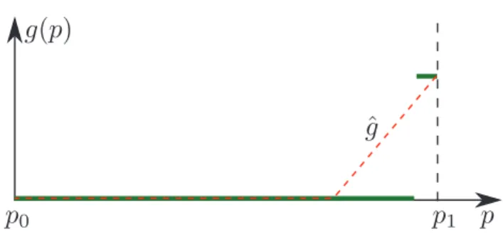
• Negative integrals estimates can be obtained even for positive functions. • It can perform worse than standard Monte-Carlo when g − ˆg contains more
variations than g (see Figure 3.1 for a 1D example).
To robustly address these two issues, we also compute, with the same samples and thus a minimal overhead, a standard Monte-Carlo estimation:
(3.4) < Im(R) >= 1 Np Np X i=1 V (R) S S X s=1 g(Pi,s) ! .
Note that here, the uniformity of the stratified samples is crucial for < Ic > and < Im> to be equally well sampled.
Fig. 3.1. Illustration of a function g for which control variate-based estimation requires a lot more samples than standard Monte-Carlo: the function (green) is constant everywhere except near p1. The control variate ˆg(red dashed) matches g for the left-most part, but leads to non-constant g − ˆgfor the right-most part, thus requiring more samples.
Once the Np passes have been performed, the final vector-valued estimation is ob-tained by taking, independently for each component, the estimation with lowest vari-ance between standard Monte-Carlo estimation and control-variate-based estimation. For a given component, if g is known to be positive for this component and the estimate of control variate is negative, the standard Monte-Carlo estimate is taken.
3.3. Convergence Criterion. The convergence of our method is based on the estimated accuracy of the estimation. For each component of the function we would like to find an estimate < I >n of the exact value Inthat satisfies:
(3.5) |< I >n−In| < ǫa or
(3.6) |< I >n−In| < ǫr× In
where ǫa is an absolute tolerance parameter and ǫr a relative tolerance parameter. As < I >n is assumed to have a Gaussian distribution with mean value In and variance σ2
n for each component n∈ {1, . . . , N}, we have: (3.7) P (|< I >n−In| < 2pσ2n) = 0.95.
Using the absolute tolerance parameter ǫa, the relative tolerance parameter ǫr and the Gaussian nature of the distribution, we define our convergence criterion as:
(3.8) 2pσ2
n< max(ǫa, ǫr× |< I >n|)) .
We therefore consider that the computation of the integral of a component converged when:
(3.9) σ2
n<
max(ǫa, ǫr× |< I >n|)2 4
where, similarly to [7], we use < I >ninstead of In because In is not known. As soon as Equation (3.9) is satisfied for all the components, the computation is stopped. As we do not know the exact variance of the Gaussian distribution of the global estimation, we use the global variance estimate to perform the convergence test. Since
this convergence criterion relies on confidence intervals, its exact interpretation is subtle. It ensures that when a large number of estimations of the same integral is done, 95% of the estimations actually respect the precision requirements.
3.4. Kd-tree as Control Variate. Our control variate is based on a kd-tree, each leaf representing the integrand with a first-order approximation. When a leaf is split into two parts, the split plane is placed at the middle of the longest axis. This allows us to associate a node of the kd-tree to each estimation.
The first-order approximation of the integrand inside a node of the kd-tree covering a regionR ⊂ Ω, of extents e1, . . . , eD in each dimension, with centroid c, is based on two quantities∇+and∇− computed using finite differences:
∇+g n(c)d= gn(c + (0, . . . , ed/2, . . . , 0))− gn(c) ed/2 (3.10) ∇−g n(c)d= gn(c− (0, . . . , ed/2, . . . , 0))− gn(c) ed/2 (3.11)
where ed/2 is the d−th component of the vector (0, . . . , ed/2, . . . , 0).
The value of the n−th component of the control variate at a point p belonging to R is then given by the integrand approximation:
(3.12) gˆn(p) = gn(c) +∇gn(c, p)· |p − c|
with∇gn(c, p)d=∇+gn(c)dif pd≥ cd, and∇gn(c, p)d=∇−gn(c)dotherwise, for the D components of∇gn(c, p). This interpolant function gives an adequate compromise between smoothness, memory storage, and evaluation cost. In the remaining, we call the N -components function defined from Equation (3.12) a gradient interpolator. The integral of this function overR for a component n is:
(3.13) Z R ˆ gn(p)dp = V × gn(c) + D X d=1 (∇+gn(c) +∇−gn(c))× ed 8 ! ,
where V is the volume of the region. The important point is that even though our approximation defines N× 2D hyperplanes, we store only 2× N × D values for ∇+ and∇−, and the integral is computed in a linear time with respect to D.
Any suitable higher-order approximation could replace the gradient interpolator. However, the use of a separable approximation instead of a tensor-product-like in-terpolation to avoid a huge memory overhead, and the tendency of higher-order ap-proximations to oscillate are likely to lead to a poor approximation. Oscillations would combine in an undesirable and uncontrollable manner when evaluating the separable approximation, introducing higher frequency in the g(p)− ˆg(p) term than what actu-ally exists in g(p), making g(p)− ˆg(p) more complicated to integrate than the original
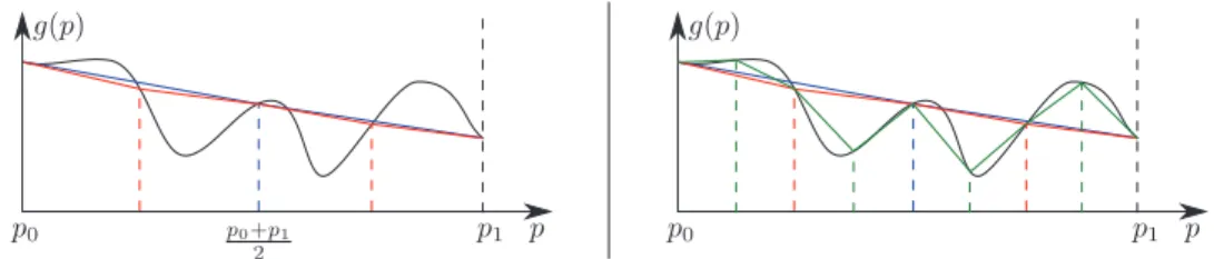
Fig. 3.2. Illustration of leaves representation and refinement: suppose a leaf covers the interval [p0, p1]. Its coarsest interpolator is in blue, and the two more precise interpolators, in red, are
obtained by cutting [p0, p1] in two halves. Here, I1is the integral of the blue interpolator, and I2is
the sum of the integrals of the red interpolators.
problem. In addition, higher-order approximations require more function evaluations for their construction, and are more costly to evaluate. For these reasons, we found the first-order approximation a good compromise between accuracy and speed, while limiting the introduction of undesired high-frequencies with arbitrary integrands. Local selective refinement: The control variate is never globally refined: refinement is applied locally on the sub-tree containing the region of interest. As most methods, our refinement is based on an approximation error [6]. As illustrated on the 1D case in Figure 3.2, our error is estimated using three gradient interpolators inside each leaf: the first covers the whole leaf and the two others cover the two halves of the region. Let I1be the integral of the coarsest gradient interpolator, and I2be the sum of the integrals of the two others. We refine the leaf if, for at least one component: (3.14) |I1− I2| > max(ǫcr× Gˆ , ǫ c a)
where ˆG is the integral of the global control variate computed before the refinement starts. We use ǫc
r = 10× ǫr and ǫca= 10× ǫato get a sufficient approximation while not being yet as precise as required for the whole estimation.
Control variate evaluation and integral: We use the two interpolators, each covering half of the region covered by a node, as ˆg function. The control variate integral in a leaf is the sum of the two interpolator integrals, and the complete control variate integral is the sum of each leaf integral.
3.5. Control Variate and Estimations Interactions. Non-combinatorial stratified sampling: The structure of our control variate directly provides the strata of our stratified sampling scheme. Indeed, the middle split strategy of our kd-tree ensures that for a nodeN , the best S = 2dstrata coveringN are the nodes at d levels below N . This way, the number of strata is constant whatever the value of D and strata are dominantly cube-shaped, providing an adequate samples distribution. The value d thus determines the robustness of the estimator, while Np determines its distribution. The combination of d and Np allows us to determine the accuracy of the estimation, as 2d
× Npsamples are used for each estimation. A good starting point to set these variables is to use Np = 15 and d = 4, which allows avoiding an important loss of samples when refining an estimation while ensuring both an
Fig. 3.3. Left: illustration of a selective refinement failure: the computed error is far from the actual error. Right: after refinement when d = 1 (leading to the green leaves), the error is correctly detected as large, and selective refinement for this node will lead to a more correct control variate.
estimator distribution close to a Gaussian and a correct stratification. We use these values for all our examples (whatever the integrand dimension or characteristics) and they can be used safely for any function to integrate.
Estimation-guided control variate refinement: The estimation of each stratum is an independent Monte-Carlo estimation. Better estimations are obtained with at least one control variate leaf per stratum. The control variate subtree with root N must thus have a minimum depth of d. If not, we refine it systematically up to depth d, and selectively afterward. This allows us to handle very difficult cases such as illustrated in Figure 3.3. In fact, this largely improves the robustness of our control variate to arbitrary-frequency content, and reduces the sensitivity of GACV to the values of ǫc
r and ǫar, as refinement occurs locally based on Monte-Carlo estimation. 3.6. Estimation Error. The globally adaptive subdivision selects the regions to split according to an error measure. It is derived from our convergence criterion (Equation (3.9)). At each step, we select the region in which the estimation is the least converged. For scalar integrands, this is done by selecting the regions according to the variance of their estimates.
For vector-valued integrands, scale differences between components have to be taken into account. A criterion based on a scale-independent error is given by:
(3.15) 4× σ
2
max(ǫa, ǫr× |< I >|)2 < 1.
As our global estimator is the sum of Gaussian estimators, one by estimation leaf, the global error is the sum of the error of each leaf relatively to the global estimate, given by:
(3.16) 4× σ
2(R) max(ǫa, ǫr× |< I >|)2
< 1.
We obtain the final scalar error from Equation (3.16) by taking the maximum over all the components.
As Equation (3.16) uses < I > which changes at each step, we have to update the errors and rebuild the heap accordingly. As this is too costly, we do not update the errors at each step. Instead, they are updated and the heap is rebuilt very often at the beginning, since the relative scales between components can change dramatically, and less often after a few iterations because the relative scales estimations are stabilized.
We thus update the errors and rebuild the heap at the second step, the fourth step, the eight-th step, and so forth.
3.7. Integrals over Arbitrary Finite-Dimensional Supports. As shown in [8], Monte-Carlo estimation can be considered as computing an integral over the unit-hypercube of uniform random numbers in [0, 1). Instead of computing the integral of a function g over an arbitrary support Ω,
(3.17) I =
Z
Ω
g(x)dµ(x)
one can use a mapping X : [0, 1)D → Ω between numbers in [0, 1)D and elements of Ω, which has the properties of a random variable defined over the uniform random hypercube of dimension D. This random variable X defines a probability distribution on Ω, and for the measure of integration µ, it has an associated probability density function pX,µ. Then, Equation (3.17) can be reformulated as an integral over a bounded axis-aligned support:
(3.18) I = Z [0,1)D g(X(u)) pX,µ(X(u)) du
where u is a D-dimensional vector of numbers in [0, 1). This general reformulation allows us to handle arbitrary supports whenever D is a finite constant and X satisfies g(x)6= 0 ⇒ pX,µ(x) > 0.
Combining GACV and importance sampling: Equation (3.18) also allows us to use GACV and importance sampling at the same time. If a well adapted sampling distribution X is known for g, integrating pX,µg(X(u))(X(u)) using GACV leads to a very effective combination of importance sampling and control variate.
4. Numerical Evaluation. In order to experimentally verify that GACV reaches our objectives (mathematical and computational robustness, efficiency, generality), we have developed a set of numerical tests and compare GACV against two variants of SUAVE: a deterministic using QMC (SUAVE-QMC) and a stochastic using a PRNG (SUAVE-PRNG).
We use SUAVE with the default numeric parameters given for the Mathematica im-plementation and we limit the maximum number of samples to 100 millions. With SUAVE, we can use only the samples in the leaves of the estimation tree, or all the samples to compute the global integral value. However, although slightly faster, this last possibility has shown to largely decrease the accuracy of the method. We thus use the leaves samples only.
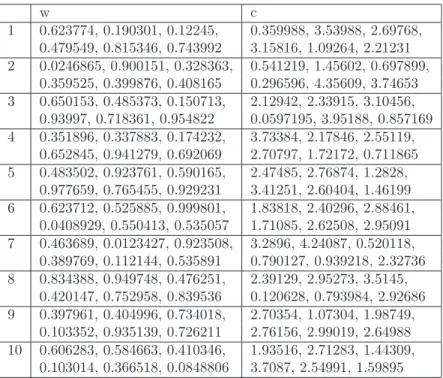
4.1. Tests Functions. Genz test functions [5]: Genz defined six families of functions to easily test the behavior of numerical integration methods with arbitrary-dimensional scalar functions. These families of functions are parameterized by two randomly chosen vectors. The first vector, denoted w, is non-affective, i.e. different values of w should lead to similar performances. The second vector, denoted c, is affective through its norm (called difficulty d): the larger the norm, the more difficult to integrate the function. For a given difficulty d, the components of w and c are first chosen randomly in [0, 1), and c is scaled so that its norm equals d. Note that for a same difficulty, different c vectors should lead to similar performances.
The test functions are defined as: Oscillatory : f1(x) = cos(c· x + 2πw1) Productpeak : f2(x) = D Y i=1 1 (xi− wi)2+ c−2i Cornerpeak : f3(x) = 1 (1 + c· x)D+1 Gaussian : f4(x) = exp(−c2· (x − w)2) C0−continuous : f5(x) = exp(−c · |(x − w)|) Discontinuous : f6(x) = 0 if x1> w1 or x2> w2 exp(c· x) otherwise
In a similar fashion to [7], we perform our tests following the process summarized in Algorithm 2. We use the same difficulty values as in [7] (d(f 1) = 6, d(f 2) = 18, d(f 3) = 2.2, d(f 4) = 15.2, d(f 5) = 16.1, d(f 6) = 16.4), and we compute integrals for ten values of w and c for each of the six Genz functions. The values used to generate the functions in the tests analyzed below can be found in Appendix A. For all functions, we set the convergence parameters of our confidence-interval-based convergence criterion (Section 3.3) with ǫr = 10−3 as ǫa= 10−7in Equation (3.9). We test the computational stability of the stochastic methods – GACV and SUAVE-PRNG – by performing 50 independent estimations of each integral. Compared to [7], we perform the test for D = 6, a middle-dimensional integration problem. In order to also evaluate the behavior of the integration methods on vector-valued integrands, we propose the use of a seventh test function family defined as fc= (f1, . . . , f6). Participating media integration: In addition to specifically designed test func-tions, we use two 3-components functions defining the scattering coefficients of two participating media represented by RGB triplets (D = 3 in this case). The rendering of these participating media with ray-marching is shown in Figure 5.1.
The first participating medium, called Porsche, is the density of a Porsche car, trans-formed by a colored transfer function. This medium is represented by a grid of 559× 1023 × 347 nodes, with a total of 193 millions cells. It exhibits a lot of details and sharp non-axis-aligned features.
The second participating medium, called cloud, has been produced using Ebert’s pro-cedural system [3]. This model exhibits both smooth parts and very-high frequencies, localized on the border of the cloud. No analytical properties are available for this function.
Our test consists in integrating the scattering coefficients on the whole support of these media with three different relative precisions: 0.1, 0.01, and 0.001. For each precision, we evaluate the robustness and the accuracy of the three methods by computing the integral, 1000 times with GACV and PRNG, and only once with SUAVE-QMC as it is deterministic.
4.2. Analysis. In our figures, we use the following color code: blue for GACV, red for SUAVE-PRNG and green for SUAVE-QMC.
For each family of scalar functions f1to f6, we consider ten different functions defined by ten different values of (w, c). For each of these functions, we perform 50 compu-tations. In plots analyzing the integration of Genz scalar test functions (Figures 4.1 and 4.4), values are organized as 6 successive blocks of 500 values: one per function family. Each block contains 10 contiguous sets of 50 values, one per function. Finally, in Figures 4.1, 4.2, 4.4, and 4.5, plots illustrating the behavior of SUAVE-QMC are presented by duplicating 50 times the result of single evaluations.
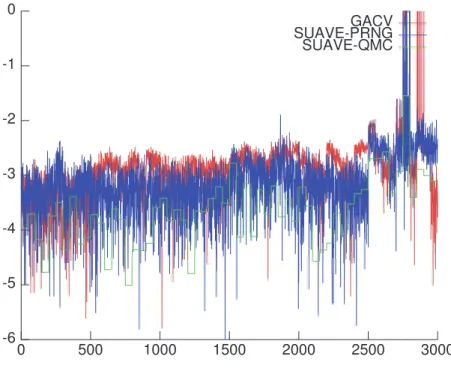
4.2.1. Accuracy and Mathematical Robustness. Scalar integrands: The accuracy of our method is confirmed by the relative errors computed from reference values, obtained with standard Monte-Carlo. Figure 4.1 presents the log10(|< I > −I| / |I|) plot for the 3000 scalar integrals computed on the Genz func-tions. All methods give results with a relative error of about 0.001, which matches the precision requirements given in Section 4.1, i.e. the relative precision ǫr is below 10−3.
As presented in Section 3.2, GACV relies on two coupled estimators: a control-variate estimator and standard Monte-Carlo. The Monte-Carlo estimator only avoids some pitfalls of the control-variate estimator, and it is therefore used for very few esti-mations in GACV. This has been verified for all our test functions: the standard Monte-Carlo estimator is used for less than 1% of the estimations, which confirms the gain provided by control-variate for variance reduction.
There is a noticeable accuracy exception both for GACV and SUAVE-PRNG, which exhibit a very large variance for one or two of the ten integrands of the family of functions f6(Figure 4.1, right), as the returned value for the integral is zero for some of the 50 computations, while others are close to the reference. In the case of GACV, this is due to an insufficiently dense sampling at the first step. Indeed, all samples may fall in the interval where f6returns 0, depending on the w1and w2values. In this case, although the w parameter should not be affective, it in fact affects the size of the non-zero interval. It is important to notice that this failure case can be detected by the large variance of several independent lower-precision estimates. When such a failure is detected, it is possible to increase the number of samples for the first few levels of estimations, or simply take the average of the non-zero estimates. SUAVE-QMC is less sensitive to such failure cases because the samples cover the integration domain very uniformly, and have thus more odds to hit the non-zero zones. However, whenever all samples are zero, there is no way to tell that the algorithm has failed: as the samples are deterministic, all estimations will give zero, while the true result is not zero and can be arbitrarily large. In this sense, methods which include a stochastic part are more helpful for arbitrary integrands because failure can be detected and dealt with.
Vector-valued integrands: Figure 4.2 presents the log10(|< I > −I| / |I|) plot for the 500 vector-valued integrals, plotting each component sequentially (first 500 points: first component, etc.). Vector-valued integrands improve GACV robustness by avoid-ing the failures appearavoid-ing in Figure 4.1. In fact, since other components require splitting, the sampling is denser for the sixth component as well.
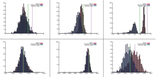
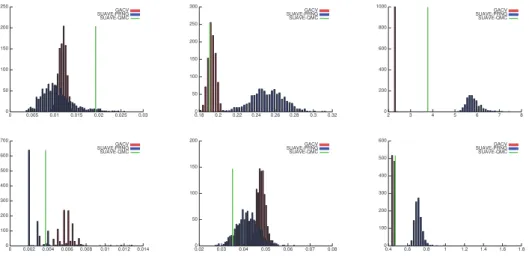
Figure 4.3 presents histograms of the 1000 integral estimations of the scattering co-efficients on the Porsche and cloud media, for the three relative precisions. Results are displayed for the third component only as the same behavior is observed on each
-6 -5 -4 -3 -2 -1 0 0 500 1000 1500 2000 2500 3000 GACV SUAVE-PRNG SUAVE-QMC
Fig. 4.1. Plot of the relative error for each scalar integrand. Ordinates are in logarithmic scale.
of them. The underestimation in the Porsche case is caused by regions where the in-tegrand is zero almost everywhere, which often lead to zero estimates and variances. However, we can see that GACV performs more accurate estimations, and better handles this case than both variants of SUAVE.
Figure 4.3 also shows that the Gaussian distribution of the estimations of GACV is in practice well verified. This validates the convergence criterion we defined in Section 3.3 and the confidence intervals we return, as both are based solely on the Gaussian nature of the distribution.
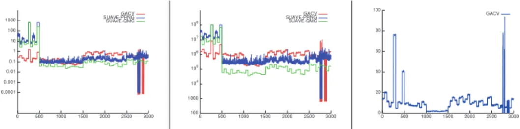
4.2.2. Efficiency and Computational Robustness. Scalar integrands: Fig-ure 4.4 contains plots of the computation time, number of evaluations required and the memory usage when available, for each scalar integrand of the Genz test. As we can see in Table 4.1, SUAVE-QMC is consistently faster than SUAVE-PRNG. It is also faster than GACV for five families of functions of the Genz test (families 2 to 6) with varying factors, but it is slower by an average factor of 100 for integrands of the first family. However, on an absolute scale, for the cases where SUAVE-QMC is faster, the absolute difference does not exceed a second, while the difference can exceed ten minutes in favor of GACV for some integrands, with computation times for GACV below 10 seconds, and in average below 0.5 seconds. Note that functions of the families f2, f4and f5are separable on all the definition domain, and that functions of the f6family are separable on the non-zero domain. This separability strongly favors SUAVE as VEGAS uses separable functions for sampling.
-6 -5 -4 -3 -2 -1 0 500 1000 1500 2000 2500 3000 GACV SUAVE-PRNG SUAVE-QMC
Fig. 4.2. Plot of the relative error for the 6 components of each integrand. Ordinates are in logarithmic scale. 0 10 20 30 40 50 60 70 80 1 1.2 1.4 1.6 1.8 2 GACV SUAVE-PRNG SUAVE-QMC 0 20 40 60 80 100 120 140 1.45 1.5 1.55 1.6 1.65 1.7 1.75 GACV SUAVE-PRNG SUAVE-QMC 0 50 100 150 200 250 300 1.64 1.65 1.66 1.67 1.68 1.69 1.7 1.71 GACV SUAVE-PRNG SUAVE-QMC 0 20 40 60 80 100 7000 8000 9000 10000 11000 12000 GACV SUAVE-PRNG SUAVE-QMC 0 50 100 150 200 8200 8400 8600 8800 9000 9200 9400 9600 GACV SUAVE-PRNG SUAVE-QMC 0 10 20 30 40 50 60 70 80 9230 9240 9250 9260 9270 9280 9290 GACV SUAVE-PRNG SUAVE-QMC
Fig. 4.3. Histograms of the values obtained for 1000 estimations with decreasing ǫrvalues (and
therefore increasing precision) on the Porsche medium (top row) and on the cloud medium (bottom row), showing only the third component of the computed integral. The green line is the value obtained by SUAVE-QMC, the magenta line is the exact integral value. Left: ǫr = 0.1, middle: ǫr = 0.01,
0.0001 0.001 0.01 0.1 1 10 100 1000 0 500 1000 1500 2000 2500 3000 GACV SUAVE-PRNG SUAVE-QMC 100 1000 104 105 106 107 108 0 500 1000 1500 2000 2500 3000 GACV SUAVE-PRNG SUAVE-QMC 0 20 40 60 80 100 0 500 1000 1500 2000 2500 3000 GACV
Fig. 4.4. Left: Time, in seconds, required by the computation of each scalar integral of the Genz test. Ordinates are in logarithmic scale. Middle: Number of evaluations required to compute each integral. Ordinates are in logarithmic scale. Right: Memory consumption with GACV, in MB.
Table 4.1
Average time, in seconds, required by each method to compute an integral for each family.
f1 f2 f3 f4 f5 f6 GACV 0.45 0.16 0.06 0.76 0.64 0.34 SUAVE-PRNG 138.51 0.10 0.11 0.23 0.17 0.34 SUAVE-QMC 96.02 0.04 0.03 0.11 0.05 0.12
Figure 4.4 also shows that GACV is very stable in terms of both computation time and number of evaluations for a same integrand, while SUAVE-PRNG exhibits large variations. The memory consumption of GACV is also stable when evaluating several times an integrand, except for the integrands where zero estimates are obtained. In this case, memory consumption is lower since these zero estimates are handled using a single node in the estimation tree.
The peak memory consumption for this test is 93MB for GACV, with a non-memory-optimal implementation. Memory consumption data is not available for SUAVE, but we did note that the memory used by our simple test program went as high as ten gigabytes of memory with both SUAVE-QMC and SUAVE-PRNG for two of the integrands of the first family (i.e. , the 100 estimations each required 10GB of memory). This peak is confirmed by the number of integrand evaluations required by SUAVE for each integral computation: the 100 millions samples limit has been reached several times by SUAVE-PRNG and SUAVE-QMC. Increasing the maximum number of samples would allow a complete estimation, at the cost of increased computation time and memory consumption.
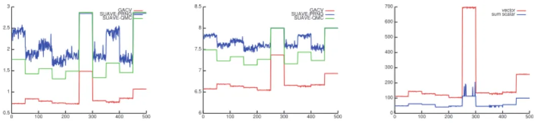
Vector-valued integrands: As in the scalar case, Figure 4.5 contains plots of the computation time, the number of evaluations required and memory usage when avail-able, for each of the 500 vector-valued integral evaluations.
A robust method for vector-valued integrand should not require more function eval-uations than the sum of function evaleval-uations required to compute each component separately. In fact, each evaluation brings informations for all components at once, leading to an automatic use of the correlation amongst components. Table 4.2 shows that this is well verified in practice for GACV when integrating functions of the fc family, while both SUAVE-PRNG and SUAVE-QMC do not benefit from any possible correlation amongst components and require a lot more evaluations than computing each component separately. This is a consequence of the use of importance sampling on weakly-correlated vector-valued integrands. The plots of number of evaluations
0.5 1 1.5 2 2.5 3 0 100 200 300 400 500 GACV SUAVE-PRNG SUAVE-QMC 6 6.5 7 7.5 8 8.5 0 100 200 300 400 500 GACV SUAVE-PRNG SUAVE-QMC 0 100 200 300 400 500 600 700 0 100 200 300 400 500 vector sum scalar
Fig. 4.5. Left: Computation time of each vector integral of the Genz test, in seconds. Ordinates are in logarithmic scale. Middle: Number of evaluations required to compute each integral. Ordinates are in logarithmic scale. Right: Memory consumption with GACV when all components are directly computed (red), and sum of the consumptions when they are computed separately (blue), in MB.
Table 4.2
Average ratio of number of evaluations required to compute fcand f1, . . . , f6separately, for the
ten different values of w and c.
GACV 0.69 0.71 0.68 0.89 0.67 1.74 0.88 0.81 0.74 0.79 SUAVE-PRNG 1.73 2.76 1.85 1.96 1.85 0.98 2.59 1.96 2.09 1.45 SUAVE-QMC 1.70 3.46 1.72 1.78 2.07 0.99 2.75 1.89 2.42 0.76
and computation times assess that GACV is also computationally stable on vector-valued functions, and much faster than both versions of SUAVE.
The right-most plot in Figure 4.5 shows that the memory used by GACV for each fc integration is larger and globally proportional to the sum of the memory used to eval-uate each component. Indeed, the adaptive control variate tree stores more elements per gradient and value at centroid than each individual control variate tree when components are computed separately. The ratio of memory consumption depends on the correlation between components, the stronger the correlation, the lower the ratio. Note that in theory, this plot does not have any per-evaluation meaning, as f1, . . . , f6 are evaluated independently of fc. However, as our memory use is stable, it allows us to visualize the proportionality for a given family of functions.
The speed and computational time stability, is also confirmed by our tests on partic-ipating media, shown in Figure 4.6. Moreover, Figure 4.6 shows that GACV exhibits a linear behavior with respect to standard deviation both for computation time and number of evaluation, while both SUAVE-QMC and SUAVE-PRNG are in between linear and the standard quadratic behavior or pure Monte-Carlo methods with re-spect to precision. For instance for the Porsche, 0.013 seconds are required by GACV in average for a relative error ǫr = 0.1, 0.19 seconds for ǫr = 0.01, and 2.3 seconds for ǫr = 0.001: the time/precision ratio (which is mathematically represented by the
product t× ǫr, as precision is inversely proportional to ǫr) is roughly constant. Mean-while, for both SUAVE-PRNG and SUAVE-QMC, the time/precision ratio largely increases when increasing the precision. This translates by the fact that even if both SUAVE-PRNG and SUAVE-QMC are faster than GACV at low precision, they be-come significantly slower when high precision is required, in a non-linear way. The linear behavior of GACV allows one to tackle high-precision problems while still re-quiring acceptable amounts of time.
0 50 100 150 200 250 0 0.005 0.01 0.015 0.02 0.025 0.03 GACV SUAVE-PRNG SUAVE-QMC 0 50 100 150 200 250 300 0.18 0.2 0.22 0.24 0.26 0.28 0.3 0.32 GACV SUAVE-PRNG SUAVE-QMC 0 200 400 600 800 1000 2 3 4 5 6 7 8 GACV SUAVE-PRNG SUAVE-QMC 0 100 200 300 400 500 600 700 0 0.002 0.004 0.006 0.008 0.01 0.012 0.014 GACV SUAVE-PRNG SUAVE-QMC 0 50 100 150 200 0.02 0.03 0.04 0.05 0.06 0.07 0.08 GACV SUAVE-PRNG SUAVE-QMC 0 100 200 300 400 500 600 0.4 0.6 0.8 1 1.2 1.4 1.6 1.8 GACV SUAVE-PRNG SUAVE-QMC
Fig. 4.6. Histograms of time, in seconds, required to compute the integral of the RGB scattering coefficients for the whole Porsche (top row) and the cloud (bottom row) media, for decreasing relative error (increasing precision). The green vertical line is the time needed by SUAVE-QMC. Left: ǫr=
0.1, middle: ǫr= 0.01, right: ǫr= 0.001.
5. Application to Voxelization of Participating Media. Volumetric ob-jects such as smoke, fog, underwater and other participating media are often repre-sented by a spatial distribution of absorption and scattering coefficients. We use RGB triplets to encode these coefficients. The light transport equation handling arbitrary media requires costly numerical integration and sampling along a ray [13]. To im-prove efficiency, the original medium is usually approximated by functions allowing analytical integration and sampling. Note that recently, sampling of arbitrary media has received a lot of attention [14, 15]. An accurate and multi-resolution representa-tion is the octree. It consists in representing the media by a tree, each intermediate node having 8 equally-sized children distributed in a regular 2× 2 × 2 grid. Each node contains an approximation of the medium within the octree node, this approx-imation being any function that can be efficiently integrated and sampled along a ray. The precision of the approximation can be efficiently controlled using an error-driven construction: the only parameter is then the maximum error ǫ allowed for the approximation. We use a quadratic error:
(5.1) E =
Z
Ω
(h(p)− f(p))2dp
where Ω is the support of the participating medium, h is the approximation, and f the original medium. This error is a 6-components error, as we have one RGB triplet for absorption and one for scattering. The construction is done using an iterative approach based on local errors: each time a node is added, its quadratic error is computed. If it is below a limit ǫl, then it is a leaf. The complete construction algorithm thus consists in first building an octree which ensures that each node has an error below the maximum global error ǫ, then computing the global error by summing each leaf local error. If this global error is below ǫ, the construction is finished. Otherwise, the octree is refined up to a local error below ǫ/2, then, if required, ǫ/4, etc., until the global error is below ǫ.
Table 5.1
Number of nodes and time needed to compute an octree representation for the Porsche and cloud media. A constant approximation is used for the Porsche medium, and a linear approximation is used for the cloud medium.
Porsche cloud
# nodes time # nodes times GACV 8258463 20m24s 1003909 5m09 SUAVE-PRNG 8409633 38m49s 1017747 6m64s
Therefore, the number of integrals to compute when building an octree is proportional to the number of nodes in the octree: there is one 6-components integral to compute the local error, and a certain number of integrals, depending on the approximation used in the leaves. We demonstrate constant and linear approximations, which both require one 6-components integral per node. This leads in general to several millions of integrals to be evaluated during the construction, for which we require a relative precision of 10−2 and an absolute precision of 10−7 in our implementation. These integrals cover a large range of integration domains, in which a large variety of inte-grands are defined (from zero almost everywhere for the empty part of the Porsche to highly irregular on the border of the cloud).
Table 5.1 shows the computation times needed to build an octree when GACV and SUAVE-PRNG are used to evaluate the integrals. The structure sizes (and number of integrals to compute) are very close, which shows that both methods give similar results for the required global error. Therefore, the lower construction time of GACV is only due to faster integral computations. The time difference for the cloud case is lower because of the complete correlation between the components, allowing the importance sampling used by SUAVE to give correct samples for all components at once. However, even in this case, GACV remains faster. In addition to the numerical validation of our method’s accuracy in Section 4, Figure 5.1 shows that the octrees closely represent the original media, visually validating the accuracy of the evaluation of the millions of integrals required to create the voxelized representation. Note that in our implementation, the octree-construction process is sequential and not paral-lelized. All the integral computations are thus done sequentially, and the maximum memory consumption for the integrals computation is the memory cost of the costliest integration. As shown in Section 4, this memory cost is low for GACV.
This last test confirms that our method is fast, accurate and stable, and is therefore well adapted for arbitrary integrands on low-to-middle-dimensional domains.
6. Conclusion. In this paper, we present globally adaptive control variate, a numerical integration method based on control variate, targeting arbitrary scalar or vector-valued integrands on low-to-middle dimensional spaces. This method relies both on deterministic quadrature rules and Monte-Carlo estimation. We propose to combine a globally adaptive subdivision and a locally-refinable kd-tree with non-combinatorial first-order approximations. We perform the estimations required by the subdivision using a novel estimator based on the control variate and standard Monte-Carlo estimation, which avoids the flaws of standard control variate. We then link the control variate and Monte-Carlo estimation, refining the control variate where needed by the estimation, and using the structure of the control variate to ensure high-quality non-combinatorial stratified sampling.
ref GACV SUAVE-PRNG
Fig. 5.1. All images are rendered with ray-marching. On the left, the reference medium, in the middle and on the right, the medium is approximated by an octree with an error of ǫ = 0.001 for the Porsche and an error of ǫ = 0.5 for the cloud. Integral evaluations for the octree construction are done with our GACV method for middle images, and with the SUAVE-PRNG method for images on the right.
Extensive numerical tests have shown that GACV is accurate, highly robust compu-tationally, fast, linear with respect to precision in practice, and requires a low amount of memory both in the scalar and vector-valued case. Further analysis has shown that GACV is particularly well-suited for vector-valued integrals, as it naturally exploits the correlation amongst components.
Adding the fact that GACV is simple to implement, this allows us to propose an effective method for the integration of arbitrary low-to-middle-dimensional scalar or vector-valued functions as, for instance, those used in the field of computer graphics. Source code: The source code of our C++ implementation is provided in the authors webpage. It can be used as a black-box integration method whose integration in a program is illustrated in an example reproducing the results of one of the tests used to analyze our method.
REFERENCES
[1] P.J. Davis and P. Rabinowitz, Methods of Numerical Integration: Second Edition, Dover Publications, 2007.
[2] R. Douc, A. Guillin, J.-M. Marin, and C.P. Robert, Minimum variance importance sam-pling via Population Monte Carlo, Research Report RR-5699, INRIA, 2005.
[3] D.S. Ebert, Volumetric modeling with implicit functions: a cloud is born, in SIGGRAPH ’97, 1997, pp. 147–154.
[4] Shaohua Fan, Stephen Chenney, Bo Hu, Kam-Wah Tsui, and Yu-Chi Lai, Optimizing con-trol variate estimators for rendering, in Proceedings of Eurographics 2006, Eurographics Association, sep 2006.
[5] A. Genz, Numerical integration – recent developments, Reidel, 1987, ch. A package for testing multiple integration subroutines, pp. 337–340.
w c 1 0.623774, 0.190301, 0.12245, 0.359988, 3.53988, 2.69768, 0.479549, 0.815346, 0.743992 3.15816, 1.09264, 2.21231 2 0.0246865, 0.900151, 0.328363, 0.541219, 1.45602, 0.697899, 0.359525, 0.399876, 0.408165 0.296596, 4.35609, 3.74653 3 0.650153, 0.485373, 0.150713, 2.12942, 2.33915, 3.10456, 0.93997, 0.718361, 0.954822 0.0597195, 3.95188, 0.857169 4 0.351896, 0.337883, 0.174232, 3.73384, 2.17846, 2.55119, 0.652845, 0.941279, 0.692069 2.70797, 1.72172, 0.711865 5 0.483502, 0.923761, 0.590165, 2.47485, 2.76874, 1.2828, 0.977659, 0.765455, 0.929231 3.41251, 2.60404, 1.46199 6 0.623712, 0.525885, 0.999801, 1.83818, 2.40296, 2.88461, 0.0408929, 0.550413, 0.535057 1.71085, 2.62508, 2.95091 7 0.463689, 0.0123427, 0.923508, 3.2896, 4.24087, 0.520118, 0.389769, 0.112144, 0.535891 0.790127, 0.939218, 2.32736 8 0.834388, 0.949748, 0.476251, 2.39129, 2.95273, 3.5145, 0.420147, 0.752958, 0.839536 0.120628, 0.793984, 2.92686 9 0.397961, 0.404996, 0.734018, 2.70354, 1.07304, 1.98749, 0.103352, 0.935139, 0.726211 2.76156, 2.99019, 2.64988 10 0.606283, 0.584663, 0.410346, 1.93516, 2.71283, 1.44309, 0.103014, 0.366518, 0.0848806 3.7087, 2.54991, 1.59895
Fig. A.1. (w, c) values used to define the ten functions of the f1 family.
[7] T. Hahn, Cuba - a library for multidimensional numerical integration, Computer Physics Communications, 168 (2005), pp. 78–95.
[8] C. Kelemen, L. Szirmay-Kalos, G. Antal, and F. Csonka, A simple and robust mutation strategy for the Metropolis light transport algorithm, in Eurographics ’02, 2002, pp. 531– 540.
[9] C. Lemieux, Monte Carlo and Quasi-Monte Carlo Sampling, Springer Series in Statistics, 2009. [10] G.P. Lepage, A new algorithm for adaptive multidimensional integration, Journal of
Compu-tational Physics, 27 (1978), pp. 192–203.
[11] N. Metropolis, A.W. Rosenbluth, M.N. Rosenbluth, A. H. Teller, and E. Teller, Equations of state calculations by fast computing machines, Journal of Chemical Physics 21, (1953).
[12] V. Pegoraro, I. Wald, and S.G. Parker, Sequential monte carlo adaptation in low-anisotropy participating media, in EGSR ’08, 2008.
[13] M. Pharr and G. Humphreys, Physically Based Rendering: From Theory to Implementation, Morgan Kaufmann Publishers Inc., 2004.
[14] L. Szirmay-Kalos, B. T´oth, and M. Magdics, Free path sampling in high resolution inho-mogeneous participating media, CGF, 30 (2011), pp. 85–97.
[15] Y. Yue, K. Iwasaki, B-Y. Chen, Y. Dobashi, and T. Nishita, Unbiased, adaptive stochas-tic sampling for rendering inhomogeneous parstochas-ticipating media, in SIGGRAPH ASIA ’10, ACM, 2010.
Appendix A. (w, c) values used for the Genz functions.
Tables A.1 to A.6 give the values of the 6D vectors w and c used in our tests to define each of the ten particular functions of each family of functions f1to f6.
w c 1 0.758702, 0.38111, 0.891593, 6.96479, 8.50633, 1.52203, 0.59196, 0.388804, 0.918741 9.28669, 9.65939, 4.61206 2 0.993727, 0.64499, 0.116133, 1.5071, 5.78368, 8.09016, 0.739159, 0.568956, 0.320116 6.75787, 11.8387, 6.08314 3 0.772715, 0.276255, 0.0966132, 6.10207, 10.1342, 8.86814, 0.44874, 0.429343, 0.285161 2.09008, 6.99219, 7.22214 4 0.23294, 0.998873, 0.21057, 6.01165, 6.53574, 13.3541, 0.44938, 0.52892, 0.281008 4.3687, 6.13182, 3.18233 5 0.914651, 0.850319, 0.322005, 4.52565, 2.45289, 12.0526, 0.876983, 0.0317087, 0.345794 0.461079, 11.4524, 4.56795 6 0.0532465, 0.00868384, 0.718525, 10.5072, 2.91006, 10.1423, 0.937794, 0.57114, 0.741881 1.09684, 6.18868, 7.92214 7 0.3951, 0.152574, 0.919073, 0.589352, 9.19601, 8.12021, 0.696949, 0.441537, 0.462203 8.68783, 4.38641, 8.85603 8 0.991166, 0.615778, 0.564681, 6.27547, 11.3925, 10.8478, 0.126063, 0.0953054, 0.415221 2.23915, 5.46595, 1.50427 9 0.267232, 0.795007, 0.715033, 7.42719, 2.66605, 8.28847, 0.630328, 0.550335, 0.341469 7.67531, 10.2884, 5.31683 10 0.545652, 0.746504, 0.515225, 1.54522, 12.7007, 0.570941, 0.143778, 0.969368, 0.0235161 2.4756, 9.53185, 7.93679
Fig. A.2. (w, c) values used to define the ten functions of the f2 family.
w c 1 0.996066, 0.376039, 0.887316, 0.96975, 0.57819, 1.08347, 0.863883, 0.384113, 0.829629 0.895827, 1.25669, 0.0979791 2 0.357602, 0.925072, 0.492768, 0.939382, 0.941855, 0.912073, 0.686974, 0.0458702, 0.626419 1.17399, 0.887412, 0.269871 3 0.849646, 0.663811, 0.234495, 0.408072, 0.61592, 1.90626, 0.371386, 0.130394, 0.890768 0.271705, 0.712046, 0.28186 4 0.0786581, 0.206641, 0.375283, 0.879728, 1.42545, 0.61059, 0.231487, 0.498165, 0.191031 0.0188361, 1.28295, 0.122625 5 0.551665, 0.839076, 0.257181, 1.28573, 0.489953, 0.200566, 0.585792, 0.438252, 0.635576 1.18735, 0.98551, 0.724968 6 0.201327, 0.0135834, 0.361581, 0.995853, 1.24566, 0.520221, 0.0388229, 0.499115, 0.148871 0.608746, 0.948288, 0.869568 7 0.495741, 0.158877, 0.766538, 1.2897, 1.18381, 1.05858, 0.429599, 0.900511, 0.382842 0.535369, 0.282418, 0.536906 8 0.0104496, 0.265362, 0.0355459, 1.12325, 1.15131, 1.18702, 0.616955, 0.100258, 0.336547 0.00633924, 0.909974, 0.125272 9 0.731722, 0.327559, 0.979216, 1.06804, 0.667819, 0.930277, 0.530678, 0.762478, 0.906587 0.171766, 1.44546, 0.518697 10 0.283046, 0.123783, 0.16976, 1.29954, 0.0369464, 0.412623, 0.457489, 0.578025, 0.521378 1.26157, 0.465032, 1.08248
w c 1 0.156412, 0.831411, 0.923117, 6.30934, 7.61251, 7.90224, 0.616536, 0.847492, 0.0726565 7.37846, 4.02335, 0.455522 2 0.0658485, 0.640748, 0.303903, 2.08299, 11.4683, 7.91985, 0.212092, 0.310862, 0.27356 2.7432, 3.5787, 3.48176 3 0.844623, 0.466398, 0.158683, 0.0280169, 7.48258, 5.97921, 0.899149, 0.504761, 0.398144 3.77368, 4.3088, 10.3195 4 0.0558923, 0.451815, 0.946229, 5.30014, 5.34048, 0.353898, 0.874125, 0.441977, 0.379471 7.21785, 2.74046, 10.7096 5 0.112105, 0.546312, 0.278645, 10.3715, 6.48753, 5.96052, 0.993842, 0.0126269, 0.359657 3.88281, 0.318275, 5.53878 6 0.725662, 0.703412, 0.237615, 5.2219, 4.05204, 0.65907, 0.780385, 0.622797, 0.859203 2.50617, 10.2409, 8.70408 7 0.374777, 0.58377, 0.33161, 2.73198, 9.00276, 2.37713, 0.548093, 0.295435, 0.844483 7.47496, 6.14236, 6.57817 8 0.405656, 0.0588116, 0.395332, 6.57124, 3.06293, 7.76751, 0.617291, 0.972787, 0.896758 9.35606, 5.49367, 0.653307 9 0.580609, 0.101322, 0.686808, 1.03936, 4.86077, 4.49374, 0.260081, 0.729378, 0.00742915 8.40651, 5.8042, 9.04327 10 0.1014, 0.220474, 0.922888, 0.385814, 10.0233, 1.19794, 0.48539, 0.605545, 0.12674 9.20775, 5.5423, 3.67275
Fig. A.4. (w, c) values used to define the ten functions of the f4 family.
w c 1 0.699375, 0.337099, 0.871819, 8.64799, 4.31424, 7.17919, 0.000552281, 0.698181, 0.64596 6.5203, 7.69509, 3.54121 2 0.823514, 0.759641, 0.911051, 6.34773, 1.79925, 6.7601, 0.944551, 0.84612, 0.452632 8.17347, 6.05731, 8.15374 3 0.713824, 0.410764, 0.0418437, 8.54249, 8.72665, 0.149624, 0.766876, 0.375302, 0.201961 0.0242227, 9.79776, 3.74998 4 0.884308, 0.0391942, 0.535062, 10.6363, 7.53445, 1.9196, 0.88745, 0.726834, 0.936557 0.527894, 0.570466, 9.22075 5 0.710651, 0.503139, 0.506865, 6.21455, 11.0014, 9.1579, 0.244169, 0.667725, 0.625358 1.61052, 2.15093, 2.91071 6 0.404809, 0.234661, 0.176505, 8.69045, 8.52838, 3.43345, 0.535546, 0.621093, 0.381746 1.04642, 8.53511, 5.02205 7 0.535115, 0.509324, 0.143797, 9.16423, 0.544608, 12.3572, 0.841992, 0.0724578, 0.397606 3.59163, 0.496033, 3.01415 8 0.151991, 0.658569, 0.0749296, 3.50677, 1.09029, 12.1249, 0.517615, 0.902215, 0.184896 9.74568, 1.72369, 0.873078 9 0.814709, 0.574238, 0.936322, 1.45015, 8.43709, 4.38327, 0.596951, 0.011037, 0.459489 3.36197, 7.8732, 9.66537 10 0.581242, 0.847791, 0.698418, 3.38784, 8.96986, 2.92174, 0.594835, 0.652784, 0.526436 6.69807, 6.47016, 8.4859
w c 1 0.436771, 0.493293, 0.259059, 1.50625, 2.42764, 7.60764, 0.137752, 0.595294, 0.875485 7.47758, 3.76944, 11.5238 2 0.347839, 0.660524, 0.733129, 2.02171, 6.94311, 7.65485, 0.344827, 0.640028, 0.745164 9.97186, 0.580807, 7.63505 3 0.590739, 0.500432, 0.543543, 0.399808, 1.78879, 9.14919, 0.149174, 0.151892, 0.677399 8.20287, 10.6605, 0.978947 4 0.66794, 0.550362, 0.187651, 12.1508, 6.24695, 7.48941, 0.217448, 0.440115, 0.307107 0.978312, 3.42574, 3.67556 5 0.0179835, 0.487045, 0.747625, 11.8462, 0.284885, 6.05758, 0.859514, 0.428717, 0.883062 2.67283, 2.94544, 8.71967 6 0.988677, 0.873975, 0.329262, 11.2553, 6.9405, 2.56681, 0.639251, 0.137602, 0.561776 4.95619, 3.90756, 6.90553 7 0.778948, 0.386086, 0.514636, 6.74786, 6.14656, 8.0325, 0.870759, 0.754161, 0.426763 3.20713, 9.54122, 4.45024 8 0.918717, 0.873334, 0.500004, 2.47032, 9.62646, 11.4787, 0.326895, 0.576678, 0.845766 3.05882, 5.37268, 0.452856 9 0.388402, 0.00858075, 0.388238, 9.2885, 6.62937, 8.21457, 0.761494, 0.424288, 0.193555 2.49354, 6.60472, 4.62773 10 0.0431003, 0.930203, 0.434156, 9.47776, 8.78537, 7.02012, 0.902293, 0.452968, 0.664225 5.89177, 4.17177, 0.742157
Algorithm 1 Top-level integration routine, computes an estimate < I > of I, and the size of the 95%-confidence interval wC of this estimate.
1: proc (< I >, wC) = integrate (g, Ω, ǫa, ǫr):
2: ˆg←initialize acv(g, Ω, ǫa, ǫr) {make a first estimate}
3: (< I > (Ω), σ2(Ω))← estimate(g, ˆg, Ω)
{Add the estimate to an error-based heap for zone selection.}
4: E← maxn=1...N(σn2)
5: pushHeap ((Ω, < I > (Ω), σ2(Ω)), E)
{For scale-independent error computations (Section 3.6)}
6: errorScaling← 1, stepNumber ← 1, stepUpdateError ← 1
7: loop 8: {test convergence} 9: σ2 max= max(ǫa,ǫr×|<I>|)2 16 10: if σ2< σ2
max for all components then
11: {The estimate satisfies the convergence criterion, finished} 12: return (< I >, 4×√σ2)
13: end if
14: {Take the estimate with largest error and improves it} 15: (R, < I > (R), σ2(R)) ← pop heap()
16: (R1,R2)←split(R)
17:
{Remove the estimate from this region}
18: < I >=< I >− < I > (R)
19: σ2= σ2− σ2(R)
20:
{Potentially update the error computation (Section 3.6)}
21: if stepUpdateError = nbSteps then
22: errorScaling← 1/σ2 max 23: recomputeHeap(errorScaling) 24: stepUpdateError← stepUpdateError ×2 25: end if 26: for i∈ {1, 2} do
27: {Perform the estimation (Section 3.5)} 28: (< I > (Ri), σ2(Ri))← estimate(g, ˆg, Ri)
{Add the estimate for this region to the global estimate}
29: < I >=< I > + < I > (Ri)
30: σ2= σ2+ σ2(Ri)
{Add this estimate to the heap, for further refinement}
31: Ei← maxn=1...N(σn2(Ri)× errorScalingn)
32: push heap ((Ri, < I >, σ2), Ei)
33: end for
34: stepNumber← stepNumber +1
Algorithm 2 Test of the behavior of Genz functions integration.
1: for i = 1 to 10 do 2: {Scalar integrands test} 3: for f ∈ {f1, . . . , f6} do 4: (w(f ), c(f ))← generate(d(f)) 5: for r = 1 to 50 do 6: computeIntegral(f, w, c, 0.001) 7: end for 8: end for
9: {Vector-valued integrands test} 10: fc= (f1, . . . , f6) 11: wc= (w(f1), . . . , w(f6)) 12: cc= (c(f1), . . . , c(f6)) 13: for r = 1 to 50 do 14: computeIntegral(fc, wc, cc, 0.001) 15: end for 16: end for
![Fig. 3.2. Illustration of leaves representation and refinement: suppose a leaf covers the interval [p 0 , p 1 ]](https://thumb-eu.123doks.com/thumbv2/123doknet/14220510.483618/10.892.198.548.188.356/fig-illustration-leaves-representation-refinement-suppose-covers-interval.webp)