Transport at basin scales: 2. Applications

(1)

HAL Id: hal-00301523

https://hal.archives-ouvertes.fr/hal-00301523

Submitted on 23 Aug 2005

HAL is a multi-disciplinary open access

archive for the deposit and dissemination of sci-entific research documents, whether they are pub-lished or not. The documents may come from teaching and research institutions in France or abroad, or from public or private research centers.

L’archive ouverte pluridisciplinaire HAL, est destinée au dépôt et à la diffusion de documents scientifiques de niveau recherche, publiés ou non, émanant des établissements d’enseignement et de recherche français ou étrangers, des laboratoires publics ou privés.

Transport at basin scales: 2. Applications

A. Rinaldo, G. Botter, E. Bertuzzo, A. Uccelli, T. Settin, M. Marani

To cite this version:

A. Rinaldo, G. Botter, E. Bertuzzo, A. Uccelli, T. Settin, et al.. Transport at basin scales: 2. Applications. Hydrology and Earth System Sciences Discussions, European Geosciences Union, 2005, 2 (4), pp.1641-1681. �hal-00301523�

(2)

HESSD

2, 1641–1681, 2005 Basin-scale transport: 2. A. Rinaldo et al. Title Page Abstract Introduction Conclusions References Tables Figures J I J I Back Close

Full Screen / Esc

Print Version Interactive Discussion

EGU Hydrol. Earth Sys. Sci. Discuss., 2, 1641–1681, 2005

www.copernicus.org/EGU/hess/hessd/2/1641/ SRef-ID: 1812-2116/hessd/2005-2-1641 European Geosciences Union

Hydrology and Earth System Sciences Discussions

Papers published in Hydrology and Earth System Sciences Discussions are under open-access review for the journal Hydrology and Earth System Sciences

Transport at basin scales: 2. Applications

A. Rinaldo, G. Botter, E. Bertuzzo, A. Uccelli, T. Settin, and M. Marani

International Centre for Hydrology “Dino Tonini” and Dipartimento IMAGE, Universit `a di Padova, via Loredan 20, I-35131 Padova, Italy

Received: 6 July 2005 – Accepted: 1 August 2005 – Published: 23 August 2005 Correspondence to: A. Rinaldo (andrea.rinaldo@unipd.it)

(3)

HESSD

Full Screen / Esc

EGU

Abstract

In this paper, the second of a series, we apply the models discussed in Part 1 to a sig-nificant case study. The nature of the catchment under study, the transport phenom-ena investigated (i.e. nitrates moving as solutes within runoff waters) and the scales involved in space and time, provide an elaborate test for theory and applications.

Com-5

parison of modeling predictions with field data (i.e. fluxes of carrier flow and solute nitrates) suggests that the framework proposed for geomorphic transport models is capable to describe well large-scale transport phenomena driven and/or controlled by spatially distributed hydrologic fields (e.g. rainfall patterns in space and time, drainage pathways, soil coverage and type, matter stored in immobile phases). A sample

Monte-10

Carlo mode of application of the model is also discussed where hydrologic forcings and external nitrate applications (through fertilization) are treated as random processes.

1. Introduction

Case studies of catchment models, in particular for brackish or lagoonal receiving wa-ter bodies, demand the prediction of event-based time distributions of pollution loads

15

within hydrologic runoff waters. This is the case, in particular, for the Lagoon of Venice where a pointed debate rages over the environmental sustainability of repeated clo-sures of the lagoon inlets needed in the long run to protect the city against catastrophic flooding under increasing relative sea level. To a fragile receiving water body, in fact, the pollution accumulated due to loads carried by hydrological waters (e.g. high levels

20

of nutrients, pesticides, metals and/or other dissolved materials in the surface and sub-surface waters that affect bioavailability) may cause a variety of problems, as one obvi-ously expects. It is particularly relevant to our modelling approach, and somewhat less acknowledged, the observation that the most of annual loads from nonpoint sources is carried by a few flood events rather than by the chronic transport of normal

hydro-25

(4)

HESSD

Full Screen / Esc

EGU one needs to predict the hydrologic response of catchments both in terms of

quan-tity and quality of waters. Most pollutants potentially threatening the health of aquatic environments derive from land-use. They enter the hydrological cycle driven by mass exchange processes between the circulating water carrier and immobile phases where polluting substances are stored, temporarily or permanently (e.g.Rinaldo and Marani,

5

1987;Rinaldo et al.,1989a;Cvetkovic and Dagan,1994;Gupta and Cvetkovic,2002; Rinaldo et al.,2005a,b;Botter et al.,2005). Transported matter, once dissolved in the runoff, is then driven along the drainage network where it may possibly be involved with other chemical or physical reactions such as decay, sorption, ion exchange with the bed sediments or hyporheic zones.

10

The theoretical framework described in part 1. of this paper is suited to investi-gate many practical issues related to nonpoint pollution phenomena and to basin scale transport and flow. For instance, transport processes occurring within the hillslopes, central in defining the features of the catchment travel time distributions even at sur-prisingly large scales (Wood et al., 1988; Botter et al., 2005), are also often chiefly

15

responsible of the mobilization and release of solutes at catchment scale (e.g.Rinaldo et al.,1989b;Botter et al.,2005). The relatively small velocities driving the water parti-cles within the hillslopes, in fact, are responsible for determining relatively large contact times between the soil and the hydrologic runoff, with pronounced implications for the resulting carrier concentration. Thus, the validity of the hypothesis of well-mixed

trans-20

port conditions (briefly, MRF from mass-response functions) is crucial to our theoretical construction, and has been recently investigated (Botter et al., 2005) by comparison with less restrictive lagrangian schemes (Cvetkovic and Dagan,1994).

In this paper, the geomorphic transport approach described in Paper 1 is employed to describe the hydrologic response and the nitrate fluxes in a hydraulically complex

25

catchment located in Northern Italy (see Fig. 1a): the Dese-Zero river basin and its tidal outlet reach, whose geomorphic and hydrologic features are well measured and documented.

(5)

HESSD

Full Screen / Esc

EGU

2. The test catchment and the hydrologic data

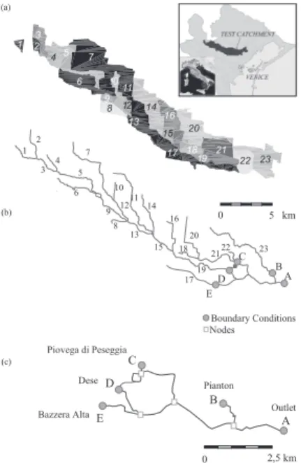
The Dese river catchment (see Fig.1) is a (roughly) 90 km2large, flat basin discharg-ing into the Venice lagoon (North-Eastern Italy). It is an elongated basin whose main-stream is about 35 km long, gemorphically characterized by groundwater-fed headwa-ters (where drainage density is low – e.g. source areas 1, 2, 3 and 23 in Fig.1b) and

5

mostly left tributaries owing to a gentle oblique slope of the Venetian plane. Such main tributaries, which drain both highly urbanized and/or extensive agricultural areas, are respectively from the mouth up, the rivers: Pianton, Piovega di Peseggia, Rio Desolino, Rio S. Martino, Rio S. Ambrogio (see Table1and Fig.1a).

In this case study, the partition between the solute and runoff generating areas and

10

the transportation zone within the hydraulic network poses no problem as it is clearly determined by the nature of the site. In fact, four drops in bottom elevation at old mill sites (see e.g. Fig.1b – sites E , D, C, B) insure critical hydraulic depths at the closure of all four basins (namely, Bazzera Alta, Dese, Piovega di Peseggia and Pianton, see Fig.1c) and, hence, a permanent transition to supercritical flow which grants the

inde-15

pendence of the upstream reach from the downstream regimes. Therefore, the tidally affected reaches of the transportation zone (shown in Fig.1c – here we do not show the tidal reach beyond the gauging site) and the hydrologic network are unambiguously de-termined regardless of the intensity of the tidal oscillations forced at the outlet. Runoff and solute fluxes are generated at the closure of the hydrologic reach via

geomor-20

phologic and mass-response function schemes. Such fluxes serve as input to routing numerical schemes of flow and transport within the tidal reach, which extends (Fig.1c) for several kilometers up to the outlet into the Venice lagoon (where gauged water el-evations are imposed as boundary conditions). Computed and measured quantities are compared at an inner gauging station (site A in Fig.1). They consist of suitable,

25

synchronous time sequences of water discharges and nitrate flux concentrations. It should be noted that boundary conditions are much affected by the tidal regime of the northern fringes of the lagoon of Venice. This microtidal environment has an area of

(6)

HESSD

Full Screen / Esc

EGU roughly 550 km2 and is characterized by a semidiurnal tidal regime with a range of

about ±0.7 m a.m.s.l. Results from recent field campaigns gathering hydrological and chemical data are available inCarrer et al. (1997); Bendoricchio et al. (1995, 1999); Zaggia et al.(2004);Collavini et al.(2005);Zuliani et al.(2005).

The model requires the subdivision of the catchment into suitable sub-basins.

Fol-5

lowing the procedure detailed in Paper 1, we recall that, typically, the size of each source area needs be larger than the correlation scale of heterogeneous properties of transport and smaller than the maximum integral scales derived from equal-time covariances of rainfall intensity fields. In such case, one treats the kriged rainfall as spatially constant within a source area, and much simplified theoretical tools apply (i.e.

10

Eqs. 25 and 26, Paper 1). The choice of subbasins is shown in Fig.1a – the average source area turned out to be roughly 4 km2. The resulting average characteristic size is O(1) km, smaller than the computed correlation length of intense rainfall which falls in the range 10–30 km (Rinaldo et al.,2003). The overall resolved drainage density is somewhat smaller than the actual one (Rinaldo et al.,2003). Note, however, that finer

15

channelizations than resolved prove immaterial to the description of the basin-scale re-sponse provided that their effect is embedded into suitable residence time distributions. Note also that in this case no digital elevation maps can be used to yield drainage di-rections along topographic steepest descent because of the flat nature of the overland areas. Since the geomorphologic path probabilities cannot be deduced from

topogra-20

phy, different types of mapping information has been carefully analyzed to obtain the whole system description (shown in Figs. 1 and 2, see Table 1 for a summary; see Rinaldo et al.,2003, for technical details.)

Available hydrologic data consisted of:

– hourly precipitation measurements available in 13 gauging stations within, and

25

in the proximity of, the study basin (provided by Consorzio Venezia Nuova, see Rinaldo et al.,2003). The average distance between any two gauges is less than 10 km, smaller than the correlation length of intense rainfall events in this zone;

(7)

HESSD

Full Screen / Esc

EGU

– meteorological information about daily solar radiation, minimum and maximum air

temperature, minimum and maximum air humidity and wind speed gauged at the standard height of 2 m, available at the same stations. These data sets constitute a database suitable for accurate computations of point values of evapotranspira-tion (provided by Consorzio Venezia Nuova, see e.g.Rinaldo et al.,2003);

5

– continuous water elevations and discharge measurements at a control section at

the outlet of the system (site A in Figs.1b and 1c) for long timespans (provided by Consorzio Venezia Nuova, see e.g.Rinaldo et al.,2003);

– field measurements of nitrate concentrations (Carrer et al.,1997;Bendoricchio et al.,1995,1999;Zaggia et al.,2004;Collavini et al.,2005;Zuliani et al.,2005) at

10

the same control section at time intervals (1 h, in a few cases 1/2 h) significantly smaller than the lead time of the hydrologic response (∼8 h) for a few events taken from elaborate field campaigns reported in the above references;

– distributed information on the different land uses are derived from extensive

databases of remotely sensed data. Image processing relies on extensive

ex-15

perience on the recognition of surface properties of hydrologic relevance in this context (Giandon et al.,2001;Marani et al.,2004).

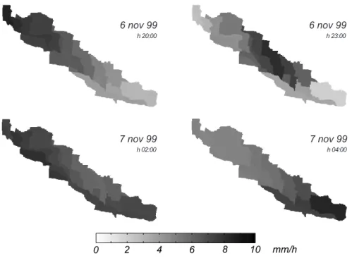
Spatially distributed information on both the rainfall fields (Fig. 4) and on the soil properties (Figs.2and3) provide a resonably complete description of the different re-gions of the basin. We employ geostatistical tools (e.g. Goovaerts, 1997) as shown

20

in Fig.4 for measured rainfall data. Kriged rainfall intensities are integrated over ev-ery source area at time steps of 1 h – see Sect. 4 and alsoRinaldo et al. (2003) for details. This allows to achieve the temporal evolution of the spatial distribution of the rainfall volumes, which in turn defines time-dependent path probabilities for all the 23 subbasins of the system, as well as their input flowrate (Part 1 – Eq. 23). Details on

25

(8)

HESSD

Full Screen / Esc

EGU The spatial distribution of soil types has been derived from published soil texture

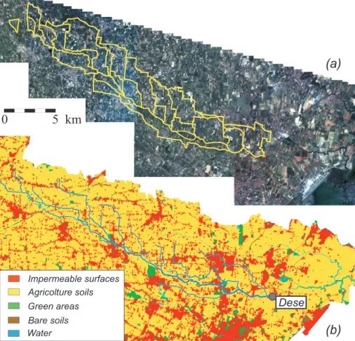
maps (Giandon et al.,2001). The catchment at hand is characterized by a highly het-erogeneous and temporally variable soil uses, typical of the developed mainland of the runoff-contributing areas to the lagoon of Venice (Figs.2and3). Different urbanization levels are observed (see Fig. 2b) and they obviously need be carefully detected

ow-5

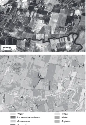
ing to the embedded, radically different processes of runoff and solute generation and transport. The use of remotely sensed data (IKONOS multispectral data, Fig.2a) and ground truths (to identify the spectral signatures of relevant soil uses and crop types) has allowed a spatially-distributed and updated description of the soil uses which exerts a fundamental control on the soil mosture dynamics and the ensuing runoff production.

10

The classification procedure adopted was based on the spectral angle mapper (SAM) algorithm (Kruse et al.,1993) and its application is shown in Fig.3. The study area has been classified by subdividing it into seven classes (urban; cropland, namely: grain, maize, soybean, wood and grass; bare soil; water). We assumed null saturated soil conductivity (Sect. 3) for water and strictly urban zones, where rainfall forcings

con-15

tribute solely to overland flow. Otherwise, the value of the saturated conductivity in the other areas has been obtained under the constraint of fixed ratios between the saturated conductivity pertaining to different land use classes. Note that we rely on literature data for the establishment of the above ratios as a function of the various soil types and/or uses (Dingman, 1994). This has clear operational advantages. In fact,

20

the number of degrees of freedom is reduced from the overall number of soil texture and land use classes, to the one corresponding to the specific value of the saturated conductivity for the reference class, which thus becomes the sole calibration parameter (Rinaldo et al.,2003).

3. Runoff production

25

An obvious source of uncertainty in models of the hydrologic response is the estimate of runoff on the basis of climate, soil use and vegetative state. A continuously updated

(9)

HESSD

Full Screen / Esc

EGU description of the instantaneous maximum infiltration rate within each source area A_γ,

say ϕ_γ(t), is achieved by the use of the Green-Ampt model for shallow soils (e.g. Ding-man,1994) (see caption of Table2). When the water-input rate J (γ, t) (see e.g. Paper 1, Eq. 23) is less than the maximum infiltration rate ϕ_γ(t) all the rainfall infiltrates into the soil (i.e. J (γ, t) becomes the actual infiltration rate). For rainfall intensities J (γ, t)

5

greater than ϕ_γ(t), instead, a rate ϕ_γ(t) infiltrates while the difference between the in-put rate and the maximum infiltration rate J (γ, t)−ϕ_γ(t) moves relatively quickly toward a stream channel (typical drainage densities relate to average unchanneled lengths that are at most a few hundred meters for this case study) and originates the short-term response of the basin. A prescribed fraction of the infiltrating volumes contributes

10

to the recharge of the water table, while the residual fraction, say η, contributes to the groundwater flow toward the channel network.

A continuously updated mathematical model has been employed in order to evaluate the evapotranspiration rates contributing to runoff production. The evapotranspiration term cannot be neglected for timescales greater than the typical duration of single

15

events, since it controls soil moisture at the beginning of each rainfall event. The model estimates the energy available to turn liquid water into vapor (which is calculated as the instantaneous atmospheric water deficit), as well as the surface turbulent transport mechanism and the vegetation transpiration constraints which concur to define the rate of vapor removal from the soil surface. Standard models of the relevant processes

20

range from empirical to sophisticated (e.g.Brutsaert,1984;Chen et al.,1996) and the choice of a suitable model must be made by balancing the overall accuracy required and the amount of information reasonably available at basin scales. We adopted the Penman-Monteith equation (e.g.Dingman,1994) integrated by the FAO approach (e.g. Allen et al.,2005), which allows a theoretically sound evaluation of evapotranspiration

25

through (relatively) few micro-meteorological, soil and vegetation parameters whose spatial distribution is determined via remotely sensed image analysis.

Evapotranspiration fluxes for an ideal reference vegetation under well-watered con-ditions and actual evapotranspiration rates of vegetation types or crops are determined

(10)

HESSD

Full Screen / Esc

EGU as in Allen et al.(2005), p. 4, Eq. (3) through the parameters reported in caption of

Table2. Note that the formulation employed properly considers also the effect of re-duced plant transpiration inre-duced by insufficient soil water contents (Allen et al.,2005; Porporato et al.,2001;Williams and Albertson,2004).

The evaluation of the seasonally changing crop characteristics, of the atmospheric

5

forcing, of the resulting soil water content and evapotranspiration are performed on a daily time scale, allowing the explicit solution of the energy and water balance with account of changes in soil use, vegetation and climate in a spatially explicit context. A synthesis of the relevant equations and parameters is reported in Table2 and in the caption.

10

Finally, plants are capable of extracting water from depths usually larger than the actual thickness of the hydrologically active soil layer (which has been estimated to be equal to 30 cm for the basin at hand, see Table2). Therefore, only a fraction σ (e.g. Williams and Albertson,2004) of the overall evaporation rates has been considered to affect the water balance within the hydrologically active top layer, while the remaining

15

part has been assumed to be drawn from deeper soil layers. The fraction of evaporated water extracted from the topsoil layer (σ) is thus the only calibration parameter for the whole evapotranspiration model and its tuning allows to reproduce the dynamics of soil depletion and the temporal variability of the water content between the storms. The long-term processes affecting the water balance within soils are responsible for

20

determining the initial water content at the beginning of each rainfall pulse (see Fig.7 for an example) where the temporal evolution of the modelled soil moisture and of the evapotranspiration flux controlling the runoff production is plotted during a sample period of about two months, which is characterized by a pronounced variability in the rainfall rates forcing the system.

(11)

HESSD

Full Screen / Esc

EGU

4. Geomorphologic hydrologic response of the Dese river system

Travel time distributions f (t) at the outlet of the four basins composing the hydrologic system (Fig.1) are obtained by a suitable decomposition over all the available paths (see Table1for the complete specification of the transitions adopted), as described in Paper 1 (Eq. 22). Path probabilities are computed in time through the relative fraction

5

of rainfall rates applied over the contributing area (Paper 1, Eq. 23). Rainfall fields are estimated by kriging point rainfall measurements (e.g. Fig. 4). The spanning set of subbasins (Fig.1), each of size considerably smaller than the macroscales of intense rainfall patterns, defines the source areas γ where spatially constant rainfall intensities

J (γ, t) are given (Paper 1, Eq. 23).

10

Most frequently used travel time pdf’s in arbitrary channel reaches c_i are exactly de-rived from proper momentum balance equations leading to an inverse gaussian form for f_c

i(t) (e.g. Rodriguez-Iturbe and Rinaldo,1997) (Chapter 7) typically dependent of

the reach length L_i, the celerity of propagation a_i and a hydrodynamic dispersion coef-ficient D_i (Table2). The residence time distribution which characterizes the hillslopes

15

response has been assumed as an exponential distribution, with a mean residence time hT_ii dependent on the hillslope area Ai, i=1→23 (Table 2, see e.g.Boyd,1978),

a relation devised for other types of terrains that nonetheless proves remarkably ac-curate in characterizing the contrasting effects of flat but deeply drained unchanneled areas (Rinaldo et al.,2003). Moreover, whether or not one needs to modify travel times

20

depending on the intensity of the hydrologic events (e.g. geomorphoclimatically) or on the modes of hydrologic transport (say when dominated by storage rather than kine-matic effects), the basic formal machinery remains unaffected as noted in Paper 1 and the above specifications suffice.

The travel time distribution within each path available for hydrologic runoff (see

Pa-25

per 1, Eq. 21) are obtained by the use of nested numerical convolutions in a discrete Fourier Transform domain, where (non-cyclic) nested convolutions of pdfs may be ex-pressed as the product of their transforms. Numerically, we employ the Fast Fourier

(12)

HESSD

Full Screen / Esc

EGU Transform (FFT) algorithm. Flow discharges (Paper 1, Eq. 24) are then obtained by

routing net rainfall impulses as obtained by the application of the water balance model (Sect. 3) to the estimated rainfall fields.

5. Mass response functions for nitrates in the Dese river

In agricultural catchments nitrogen (N) is stored and leached mainly in the form of

ni-5

trates (N-NO−₃). In the context at hand, nitrate loads carried by hydrologic runoff mainly derive (directly or indirectly) from fertilizations routinely applied onto soil surfaces by agricultural practices. Throughout this exercise we shall assume that external inputs of matter (i.e. through fertilization) becloud nitrogen cycling contributions. Because NO−₃ is highly soluble under ordinary conditions, nitrates are chiefly stored in the soil

10

moisture within immobile regions, and may be thus transferred to the circulating water carrier. As a result, nitrates are leached by hydrologic runoff, possibly causing serious damages to the ecosystem (soil acidification, O₂impoverishment, eutrophication).

One thus wonders what is the proper reaction kinetics for the description of such processes at basin scales. Specifically, we wonder whether contact times between

15

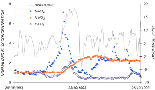
mobile and immobile waters drive solute mass transfer, and whether such process is fast or slow with respect to characteristic times of the hydrologic response, that is, mean residence times within source areas. Figure (5) shows typical field evidence from simultaneous measurements of discharges and flux concentrations of nitrates (N-NO₃), ammonia (N-NH₄) and phosphates (P-PO₄), normalized to their initial values, at

20

the gauging station for a sizable flood event (Carrer et al.,1997; Bendoricchio et al., 1995,1999). From the important facts shown therein (and from the bulk of field data e.g.Zaggia et al.,2004;Collavini et al.,2005;Zuliani et al.,2005) we deduce that:

– significant chromatographic effects appear for nitrogen compounds, but possibly

not for phosphates. Nitrates show a large delay with respect to the peak of the

hy-25

(13)

HESSD

Full Screen / Esc

EGU phases has a characteristic time larger than the lead time of runoff;

– ammonia and phosphates are sorbed onto soil particles, and are released by

desorption processes. This is not the case, however, for nitrates which are chiefly solute in soil moisture and mobilized by physical and chemical processes driven by instantaneous differences of mobile and immobile concentrations.

5

Therefore nitrates show features that are similar to those of a reactive compound. We thus propose to employ the formal machinery described in Part 1 for reactive solutes although in a somewhat different context with respect to sorption/desorption processes, and rely on the comparison of computed and measured fluxes to assess its validity. The term N(t)/k_Din Eq. (12) (Part 1) here becomes the concentration in immobile phases,

10

while the partition coefficient k_D becomes an average coefficient responsible for the transformation of N-NO₃mass into nitrate concentration in the immobile phase.

The basin-scale nitrate flux produced by an arbitrary sequence of rainfall is derived on the basis of the travel time distribution within each state, f_x

i, following the MRF

approach described in Paper 1 (see Sect. 2, Eqs. 16 to 18). In order to model the

15

solute transport within the source states where solute generation occurs A_i, i=1, 23, three different model (A–C) have been employed. A 2-layer approach (A) considers any hillslope as composed by a topsoil layer (where both infiltration and overland flow occur) and a subsurface layer (where the groundwater transport take place). Two in-dependent mass balances within the layers of each hillslope must be employed to

20

determine the temporal evolution of the nitrates mass in immobile phase. This requires to estimate the mass flux from the topsoil to the deeper layer as well as the mass ex-change rate between the mobile and the immobile phases of each layer. The latter has been computed assuming linear and rate-limited reactions, thus allowing the use of Eq. (12) of Paper 1. Note that two independent sets of reaction parameters (the

25

initial nitrate concentration in immobile phase N(0)/k_D(Paper 1, Eq. 12), and the mass transfer rate k) should be employed in order to account for the different dynamical and chemical conditions characterizing the transport within the surface and the sub-surface

(14)

HESSD

Full Screen / Esc

EGU layers. The second model (B) considers each source area as a single layer (whose

depth is equal to the sum of the thickness of the surface and of the sub-surface layers) wherein both the overland and the groundwater flows are simultaneously exchanging mass to/from immobile phases. In the latter case, one needs to carry out a single mass balance in time, so as to determine the instantaneous fraction of matter stored

5

in immobile phases. It should be noted that the instantaneous nitrate concentration in the immobile phase of each source, N_A

i(t)/kD, is crucially assumed to solely depend

on time t (Botter et al.,2005). Numerically, the temporal evolution of the mobile resi-dent concentration within the i −th source area, C_A

i(τ, t0), is obtained via an iterative

predictor-corrector finite difference scheme where, at each iteration, the unknown value

10

of N_A

i(t) (which actually depends on the solution C) is progressively updated through

a global mass balance based on the values of C obtained at the previous iteration. The above approach ensures a good efficiency in term of computational costs, regard-less of the time step employed. Initial conditions for the reaction equation, N_A

i(0), are

assumed proportional to the agricultural fraction within each subbasin (see Fig.2b –

15

Table1), thus allowing the estimate of the initial distribution of nitrates concentration in the immobile phase on the basis of a single calibration parameter (the average nitrates mass for unit agricultural surface N_a(0)). For the sake of simplicity the parameters

k and k_D have been assumed constant and spatially uniform throughout the basin. The third model (C) assumes the local equilibrium assumption (L.E.A.) within mobile

20

and immobile concentrations (C∼N(t)/k_D) that correspond to instantaneous reactions (k→∞). This model helps in determining the conditions corresponding to the case when the hydrologic runoff instantaneously dilutes all the nitrate mass stored in the control volume.

We also assume that every source state is followed by a sequence of non-reactive

25

states x₂,x₃, ..., x_k. This assumption derives from early applications of the more in-volved procedure (Paper 1, Eq. 28) where the solutes transported are actually retarded owing to chemical processes occurring with other immobile phases, e.g. bed sediment or dead zones that define chemical, biological or physical reactions). Owing to the

(15)

HESSD

Full Screen / Esc

EGU relatively small residence times of the hydrologic carrier within the channeled states

(O(1) h 1/k), however, the effects of possible reactive components acting within the channels result negligible, thus allowing the simplified approach described by Eq. (27) of Paper 1.

Path probabilities, state transitions which define the geomorphic structure of the

5

basin and the travel time distributions f_A

k(t), fck(t) within unchanneled and channeled

states are the same used for flow prediction without any tuning. This is probably the single most important operational advantage of the proposed procedure as the bulk of solute lifetime distributions (Eq. 26 of Paper 1.) is provided by independently assessed travel time distributions.

10

6. Linking runoff-generating and transportation zones

We have already noticed that the subdivision between the solute and runoff generating areas and the transportation zone within the hydraulic network is clearly determined by the nature of the site. Since both the discharges and the nitrate concentrations have been measured at the outlet of Dese (Sect. A, Fig.1c), where the effect of the

15

tidal fluctuations is not negligible (it routinely inverts even the direction of ebb/flood flows), the description of the system response required the coupling of two distinct transport models: a geomorphological-based catchment model (Sects. 4 and 5) in order to evaluate the runoff production and the nitrogen loss from the agricultural soils of the four basins, and a subsequent one-dimensional flow and transport numerical

20

model accounting for the convection and dispersion phenomena occurring within the reaches actually affected by the tidal fluctuations.

Numerical solution of the flow and transport equations suitably discretizes the main reach between the hydrological outlet of the four basins (Sect. D, Fig. 1c, the hy-drologic outlet of the Dese basin; node E in Fig. 1c, for the lower tributary Bazzera;

25

Sect. C, Fig. 1c, for a complex partition of the hydrologic contribution from the Dese river (Rinaldo et al., 2003) and the hydrologic contribution for the tributary Peseggia;

(16)

HESSD

Full Screen / Esc

EGU and Sect. B, Fig.1c, for the contribution of Rio Pianton – see also details in Table1)

and the node of Dese (node A in Fig.1c), which is the outlet of the whole system. Flow boundary conditions are given as forcing water elevations in sections A (Fig.1c) and as forcing discharges at the upstream node of the tidal network (Fig.1c). The geometry of the tidal reach is described elsewhere, as well as details of the numerical code, a

5

standard second-order time marching scheme with a suitable leapfrog spatial resolu-tion (Rinaldo et al.,2003). The result is a discretized set of water depths and velocities computed in discrete time at suitable cross sections.

Transport in the tidal reach requires numerical integration of mass balance equa-tions. Details aside (see, for technical details,Rinaldo et al.,2003), we simply recall

10

that the governing equation for the cross-sectional averaged nitrate flux concentration needs be solved along a discretized curvilinear coordinate aligned with the longitu-dinal axis of the channel. The governing equation is a convection-dispersion model where the main ingredients are: i) the velocity field, directly obtained by the unsteady flow model described above; and ii) an appropriate longitudinal, shear-flow

hydrody-15

namic dispersion coefficient, assumed constant as appropriate for mature dispersion processes owing to the much longer longitudinal distances to be covered with respect to vertical and/or transverse mixing lengths (Rinaldo et al., 2003).

Boundary and initial conditions require some attention and a few additional assump-tions. Specifically:

20

– initial concentrations along the tidal reach need to be assumed. A base

concen-tration is assumed almost arbitrarily, because the continuous nature of the model allows actual simulations to forget memory of initial conditions which rapidly be-come immaterial;

– solute fluxes are specified at the input nodes B, C, D, E as given by Eq. (26) of

25

Paper 1. applied to the four subbasins (Dese (D), Peseggia (C), Bazzera (E) and Pianton (B)). Here we assume that the mass flux of hydrologic origin is purely convective, thus neglecting the input diffusive flux at the nodes where the

(17)

bound-HESSD

Full Screen / Esc

EGU aries are imposed. This is strongly supported by hydraulic partitions of runoff

generation and transportation zones;

– at the downstream boundary (node A in Fig. 1) where one imposes the water elevations, we need to assume the trapping/pumping exchanges with the down-stream water – no simple matter for a general coupled system. Observational

5

evidence (see comparatively Figs.8and9to10) shows that the strong time vari-ability of tidal water fluxes (that often changes sign) is not paralleled by nitrate concentrations. We thus rule out the possibility that ebb flows are returned clean (say C(A, t)=0 if the pertinent flow velocity is negative (i.e. landward)). Our choice of seaward boundary condition is thus ∂C(x, t)/∂x|_x_=A=0 ∀ t, whose impact on

10

the numerical results has been deemed acceptable (Sect. 7).

The governing boundary value problem described above has been solved with a suit-able numerical scheme, which is suit-able to adjust the time step accordingly with the expected accuracy and uses efficient preconditioned conjugate gradient-like methods (Gambolati et al.,1994). Issues on the algorithms employed can be found elsewhere

15

(Rinaldo et al.,2003).

Correspondingly, sample Penman-Montieth model results are shown through the evapotranspiration terms, which affects the water mass balance within the soil between subsequent rainfall events (Fig.7).

7. Results and discussion

20

Calibration is pursued by reproducing measured discharges and nitrate concentrations at the outlet of the basin (node A in Fig. 1c). The flow and transport models are calibrated separately and on different flood events: the available data sets (see Sect. 2) consists of frequently sampled measured discharges (at hourly time step) from 1 April 1999 to 31 May 2000 and of two sets of measured nitrate concentrations sampled every

(18)

HESSD

Full Screen / Esc

EGU half-hour, from 20 October to 12 November 1993 (Carrer et al.,1997;Bendoricchio et

al.,1999), and from 25 March to 20 May 2000 (Zuliani et al.,2005).

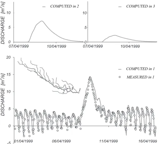
The calibration of the flow model has been performed on the event of April 1999 (see Fig.6), which is characterized by a peak discharge of 15 m3/s. An accurate description

of the rainfall volume applied to the basin, together with a fine tuning of the parameters

5

controlling runoff production (e.g. hydraulic conductivity, initial soil moisture, soil water content at the field capacity, soil thickness and the infiltrated water that contributes to short term stream response), enables a reasonably correct (and solidly reliable in time) evaluation of the volumes producing the flood. Note that the mathematical model allows to establish a close link between the parameters controlling the processes of infiltration

10

and the different soil uses. The measured hydrograph both during the ascending and the descending limbs is described reasonably well, as shown by Fig.6, where we show computed and measured discharges at the outlet of the whole system (node 1 in Fig.6, lower graph). Figure6(upper plots) also shows the computed discharges at the outlet of two different ungauged sub-basins: the Dese and the Peseggia catchments (nodes

15

2 and 3 of Fig.6, respectively).

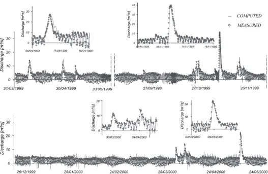
The predictive capabilities of the hydrological model is tested through a long term simulation of the response of the system to meteorological forcings from April 1999 to May 2000 (Fig.8). Non-stationary conditions in the model include seasonal variability of parameters that are described in Table2. Figure8shows the substantial agreement

20

of the modelled and the measured water discharge during the considered period, both during major rainfall events (which are reported in the insets) and within dry periods when tidal fluctuations significantly affect flows and hydrometric levels at the outlet. We thus conclude that the carrier is well understood.

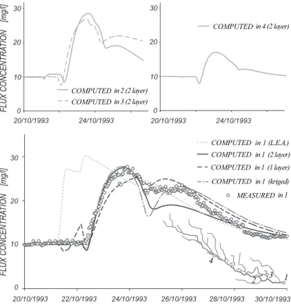
The transport model requires the calibration of three additional parameters (see

25

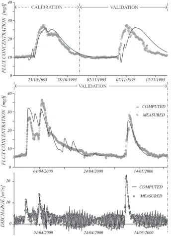
Eq. 18 of Paper 1): the parameters k and k_D and the initial nitrate mass per agri-cultural unit surface, N_a(0). We calibrate both the 2-layer and the single-layer reactive transport models on the basis of the N-NO₃ measurements collected during the event of October 1993. Figure9shows the resulting computed and measured flux

(19)

concentra-HESSD

Full Screen / Esc

EGU tions at the outlet (bottom inset). The flux concentrations computed at node 4 (upper

right inset) and at the outlets of the Dese and of the Peseggia basins (nodes 2 and 3, upper left inset) via the 2-layer model are also provided. The resulting calibration parameters for the 2- and the single-layer models are shown in Table3. As shown by Fig.9a good agreement between the computed and measured nitrate concentrations

5

at the outlet is achieved. Figure 9 also shows a comparison between the measured NO₃concentrations and the results of the L.E.A. model (C). The delay of the measured breakthrough curve with respect to the temporal evolution of the nitrates concentrations from model (C) suggests that slow mass releases from relatively immobile regions of the hillslopes indeed to determine a reactive-like behaviour (see Fig. 5). The results

10

shown in Fig.9also suggest that the 1-layer model does well in reproducing the main characters of the solute response, because the agreement between the computed and measured N-NO₃concentration is acceptable. The 2-layer approach provides an im-proved accuracy during the first days of the event at the cost of an increased number of parameters. Figure9 also shows the effects of the spatial variability of the rainfall

15

pulses on the computed nitrogen flux concentration at the outlet. The heavier tail of the hydrograph during the last four days of the event leads to a generalized increase of nitrate concentrations. This suggests that the estimate of the total runoff volume plays a major role in shaping the flux concentrations during intense rainfall event, rather than the details of its spatial distribution.

20

The validation of the nitrogen transport model has been achieved by running the model during two different periods: i) a 20-day span which closely follows the calibra-tion event (from 20 October to 15 November), and ii) a 2-month period during the spring of 2000. The initial nitrate mass for the event of November 1993 has been derived as the residual mass stored in the control volume at the end of the calibration event,

25

while for the second run (spring 2000) we tuned N_a(0) only at the beginning of the whole simulation period (25 March) without any further tuning. From the comparison between the measured and the computed N-NO₃ concentration during the validation period (Fig. 10), one may notice the satisfactory performance of the model, in

(20)

par-HESSD

Full Screen / Esc

EGU ticular for what concerns the maximum flux concentrations and for the N-NO₃ loads

transferred to the Venice lagoon. Nethertheless, in some cases the model also exhibits a certain inaccuracy in reproducing the timing of the solute release (event of Novem-ber 1993, Fig.10a) or details of breakthrough curve (event of April 2000, Fig. 10b). This may be possibly due to a variety of sources: effects of the the flushing of

pre-5

existing water characterized by low flux concentrations possibly totally denitrified; or to nitrogen cycling byproducts that we currently consider negiglible. Note finally (Fig.10) the complexity of the carrier hydrologic flowrates and the contrast with the regularity of simoultaneous nitrate concentrations, both of which are described well by our tools in a predictive mode.

10

Up to now we have omitted the effects of the long-term variability in the nitrate con-centration within the soils, which is related to slow physical and chemical processes, like mineralization, denitrification due to anaerobic bacteria and plant uptake, a step possibly leading to grossly misled predictions in other contexts. However, relatively simple empirical models may be adopted in predicting long term variations of the nitrate

15

mass between two subsequent rainfall events for different temperatures and soil con-ditions. In a sample Montecarlo simulation reported in Fig.11, we show a six-month sample period during which both the intensities and the temporal distribution of the rainfall has been reproduced through a cluster-based stochastic rainfall model of the Bartlett-Lewis type, see e.g.Rodriguez-Iturbe et al.(1987), capable of reproducing the

20

statistical properties of the observed climate. The inter-arrival time between the events and the rainfall intensities are sampled by a Poisson distribution with monthly variable parameters, so as to account for the seasonal variability of the rainfall processes. By coupling the continuous rainfall model with a relatively simple empirical model account-ing for the long-term evolution of the nitrate mass within the basin surfaces (for details,

25

see e.g.Rinaldo et al., 1989b) we simulate the nitrate discharge and the time evolu-tion of the nitrate mass stored within the catchment surfaces during the sample period. In Fig. 11 we show the sequence of simulated rainfall intensities generated with the Bartlett-Lewis model (a), the mass discharge at the outlet of the Dese basin (node D

(21)

HESSD

Full Screen / Esc

EGU of Fig.1) (b) and the pertinent temporal evolution of immobile nitrate mass (c). The

simulation reported in Fig.11considers two different scenarios: i) an initial nitrate con-tent N_a(0) of 100 [kg/ha], without any further input during the whole simulation period (solid line) and ii) an initial nitrate load of 100 [kg/ha], followed by a single fertilization (30 [kg/ha]) at the end of June (dotted line). Obviously, the second strategy leads to

5

higher mass discharges, with an increase of the nitrate mass stored in the catchment at the end of the simulation. Needless to say, more refined scenarios where both the nitrates loads and the temporal sequence of the fertilizations are treated as random variables may be included within the above framework. This would require a suitable parametrization of many bio-geochemical processes relevant for soil nitrogen cycling.

10

The above framework is designed to estimate, in a proper Montecarlo framework, the return period of the N − NO₃ loads on the basis of the maximum load generated dur-ing every simulated year. The model developed in these Papers may thus support planning strategies for sustainable land use through reduced environmental impacts of nitrate leaching to fragile ecosystems.

15

8. Conclusions

The following conclusions are worth emphasizing:

– We have applied the organized body of theory presented in paper 1 of this series

to a complex watershed where predictions of event-based pollution releases pose challenges and opportunities. The case study is particularly relevant for the

com-20

plex hydraulic conditions, the wide-ranging field observations of both flows and flux concentrations, the importance of the estimation of event-based releases in the management of the planned regulation of the receiving water body (the lagoon of Venice) and the rapidly changing land use scenarios for the entire area;

– the geomorphologic scheme of the hydrologic response works nicely in

conjunc-25

(22)

HESSD

Full Screen / Esc

EGU hydrologic scheme has been calibrated, the model runs continuously in time

pro-ducing almost indistinguishable computed and measured runoffs at the gauging station;

– the mass-response function scheme devised for the description of basin-scale

transport in the Dese River assumes that each of the 23 sources areas in which

5

we have subdivided the 90 km2area is generating solute mass through reversible, first-order reactions where the mass stored in immobile phases is proportional to the fraction of agricultural area. Notwithstanding the major simplifications intro-duced, the model results are satisfactory and suggest a noteworthy potential of the proposed approach for large-scale applications where distributed approaches

10

pose almost unsurmountable problems of parameter calibration for reliable con-tinuous predictions;

– a final section has illustrated the potential of the theoretical tools. In particular,

continuous modeling and land-use impact have been investigated within a Mon-teCarlo framework where rainfall and fertilization forcings are treated as random

15

processes (i.e. Poisson interarrivals characterized by exponential intensity). We thus conclude that mass-response function approaches are suited to describe com-plex basin-scale transport processes driven by the hydrological response.

Acknowledgements. This research is funded by the EU Project AQUATERRA (GOCE 505428). Financial support provided to GB and MM by CORILA (Consorzio per la Gestione del Centro di

20

Coordinamento delle attivit `a di Ricerca inerenti il Sistema Lagunare) (grant 3.17/2004) is grate-fully acknowledged. The writers wish to thank CONSORZIO VENEZIA NUOVA for providing the hydrologic data from a comprehensive database for the area. The writers wish to thank M. Putti, University of Padua, for providing the numerical code solving the convection-dispersion equa-tion used in computing transport in the tidal regime. Field data for nutrient releases have been

25

provided by the late G. Bendoricchio, whom we sorely miss, and by CONSORZIO VENEZIA NUOVA and Magistrato alle Acque di Venezia through their DRAIN project.

(23)

HESSD

Full Screen / Esc

EGU

References

Allen, R. G., Pereira, L. S., Smith, M., Raes, D., and Write, J. L.: FAO-56 dual crop coefficient method for estimating evaporation from soil and application extensions, J. Irrigation Drainage Eng. ASCE, 131, 2–13, 2005. 1648,1649

Bendoricchio, G., Zingales, F., and Carrer, G. M.: Verifica sperimentale di un modello di

sim-5

ulazione dei carichi di nutrienti all scala di bacino, Ingegneria Ambientale, 24, 5–12, 1995.

1645,1646,1651

Bendoricchio, G., Carrer, G.M., and Calligaro, L.: Consequences of diffuse pollution on the water quality of rivers in the watershed of the lagoon of Venice, Wat. Sci. Tech., 39, 113– 120, 1999. 1645,1646,1651,1657

10

Botter, G. and Rinaldo, A.: Scale effects on geomorphologic and kinematic dispersion, Water Resour. Res., 39, 1286–1294, 2003.

Botter, G., Bertuzzo, E., Bellin, A., and Rinaldo, A.: On the Lagrangian formulations of reac-tive solute transport in the hydrologic response, Water Resour. Res., 41, 4008–4016, 2005.

1643,1653

15

Boyd, M. J.: A storage routing model relating drainage basin hydrology and geomorphology, Water Resour. Res., 14, 921–928, 1978. 1650

Brutsaert, W.: Evaporation into the Atmosphere. Theory, History and Applications, Kluwer Aca-demic publishers, New York, 1984. 1648

Carrer, G. M., Calligaro, L., Comis, C., and Zingales, F.: Analisi in continuo dei nutrienti versati

20

nella Laguna di Venezia dal fiume Dese, Atti dell’ Accademia Patavina di Scienze, Lettere ed Arti, 60, 21–32, 1997. 1645,1646,1651,1657

Chen, F., Mitchell, K., Schaake, J., Xue, Y. K., Pan, HL., Koren, V., Duan, QY. Ek. M., and Betts, A.: Modeling of land surface evaporation by four schemes and comparison with FIFE observations, J. Geophys. Res. – Atmosphere, 101, 7251–7268, 1996. 1648

25

Collavini, F., Bettiol, C., Zaggia, L., and Zonta, R.: Pollutant loads from the drainage basin to the Venice Lagoon (Italy), Environ. Int., in press, 2005. 1645,1646,1651

Cvetkovic, V. and Dagan, G.: Transport of kinetically sorbing solute by steady random velocity in heterogeneous porous formations, J. Fluid Mech., 265, 189–215, 1994. 1643

Dingman, S. L. M.: Physical Hydrology, MacMillan, New York, 1994. 1647,1648 30

Gambolati, G., Pini, G., Putti, M., and Paniconi, C.: Finite element modelling of the solute transport of reactive contaminants in variably saturated soils with LEA and non-LEA sorption,

(24)

HESSD

Full Screen / Esc

EGU Env. Modelling, 2, 173–212, 1994. 1656

Giandon, P., Ragazzi, F., Vinci, I., Fantinato, L., Garlato, A., Mozzi, P., and Bozzo, G. P.: La carta dei suoli del bacino scolante in Laguna di Venezia, Bollettino della Societ `a Italiana della Scienza del Suolo, 50, 273–280, 2001. 1646,1647

Goovaerts, P.: Geostatistics for Natural Resources Evaluation, Oxford University Press, New

5

York, 1997. 1646

Gupta, A. and Cvetkovic, V.: Material transport from different sources in a network of streams through a catchment, Water Resour. Res., 38 1098, 2002. 1643

Kruse, F. A., Lekoff, A. B., Boardman, J. W., Heiderbrecht, K. B., Shapiro, A. T., Barloon, P. J., and Goetz, A. F. H.: The Spectral Image Processing System (SIPS) – Interactive

Visualiza-10

tion and Analysis of Imaging Data, Remote Sensing Env., 44, 145–163, 1993. 1647

Marani, M., Lanzoni, S., Silvestri, S., and Rinaldo, A.: Tidal landforms, patterns of halophytic vegetation and the fate of the lagoon of Venice, J. Mar. Systems, 51, 191–210, 2004. 1646

Porporato, A., Laio, F., Ridolfi, L., and Rodriguez-Iturbe, I.: Plants in water-controlled ecosys-tems: active role in hydrologic processes and response to water stress – III. Vegetation water

15

stress, Adv. Water Resour., 24, 725–744, 2001. 1649

Rinaldo, A. and Marani, A.: Basin scale model of solute transport, Water Resour. Res., 23, 2107–2118, 1987. 1643

Rinaldo, A., Bellin, A., and Marani, A.: On mass response functions, Water Resour. Res., 25, 1603–1617, 1989a. 1643

20

Rinaldo, A., Marani, A., and Bellin, A.: A study on solute NO₃-N transport in the hydrologic response by a MRF model, Ecol. Modelling, 48, 159–191, 1989b. 1643,1659

Rinaldo, A., Marani, M., Cudini, E., and Uccelli, A.: Studio Idrologico generale e modello con-tinuo del sistema idraulico Dese-Zero, Tech. Rep. 7-2003, International Centre for Hydrology ”Dino Tonini”, Universit `a di Padova, 148 pp., 2003. 1645,1646,1647,1650,1655,1656 25

Rinaldo, A., Bertuzzo, E., and Botter, G.: Nonpoint source transport models from empiricism to a coherent theoretical framework, Ecol. Modelling, 184, 19-35, 2005a. 1643

Rinaldo, A., Botter, G., Bertuzzo, E., Settin, T., Uccelli, A., and Marani, M.: Transport at basin scales 1. Theoretical Framework, Hydrol. Earth Syst. Sci., 2, 1613–1640, 2005b,

SRef-ID: 1812-2116/hessd/2005-2-1613. 1643

30

Rodriguez-Iturbe, I., Cox, D. R., and Isham, W.: Some models for rainfall based on stochastic point processes, Proc. Royal Soc. Lond., A410, 269–288, 1987. 1659

(25)

Cam-HESSD

Full Screen / Esc

EGU bridge Univ. Press, New York, 1997. 1650

Williams, C. A. and Albertson, J. D.: Soil moisture controls on canopy-scale water and carbon fluxes in an African savanna, Water Resour. Res., 40, W09302, 2004. 1649

Wood, E. F., Sivapalan, M., Beven, K., and Band, L.: Effects of spatial variability and scale with implications to hydrological modelling, J. Hydrol., 102, 29–47, 1988. 1643

5

Zaggia, L., Zuliani, A., Collavini, F., and Zonta, R.: Flood events and the hydrology of a complex catchment: the drainage basin of the Venice Lagoon, Coast. Environ. V, vol. 68, WIT press, Wessex (UK), 2004. 1645,1646,1651

Zuliani, A., Zaggia, L., Collavini, F., and Zonta, R.: Freshwater discharge from the drainage basin to the Venice Lagoon (Italy), Environ. Int., in press, 2005. 1645,1646,1651,1657

(26)

HESSD

Full Screen / Esc

EGU Table 1. Geomorphic transitions for the transport model. The transitions refer to the legenda

of Fig. 1. Source areas are numbered in Fig. 1a and channels are labeled in the top inset. For every channel state, ck, we have collected hydraulic, topographic and geomorphic information

that allows the uncalibrated determination of the k-th reach length, Lk, the reach slope, bankfull

width and depth (Rinaldo et al., 2003). From such information we derive information usable by the geomorphic scheme to derive the travel time distributions fc_k(t) and fA_k(t), k = 1, 23, where

the hydraulic parameters are the (bankfull) celerity of propagation, say ak and the average

hydrodynamic dispersion Dk for the channels (Table2) and a single coefficient, µ, relating the

average residence time hTki to the area Ak (Table2). Details on the geometrical and hydraulic

parameters are not reported for brevity and are available upon request (see e.g. Rinaldo et al., 2003).

Source area Geomorphic transitions Legenda

Dese - Origins A₁→ c₁→ c₃→ c₅→ c₉→ Area= 0.64 km2

(1) c₁₃→ c₁₅→ c₁₉→ D Fraction of cropland= 62% Musoncello A₂→ c₂→ c₃→ c₅→ c₉→ Area= 0.77 km2

(2) → c₁₃→ c₁₅→ c₁₉→ D Fraction of cropland= 71 % Fossetta A₃→ c₃→ c₅→ c₉→ c₁₃→ Area= 2.41 km2

(3) → c₁₅→ c₁₉→ D Fraction of cropland= 62% Rio Bianco A₄→ c₄→ c₅→ c₉→ c₁₃→ Area= 2.08 km2

(4) → c₁₅→ c₁₉→ D Fraction of cropland= 59% Piovega di Levada A₅→ c₅→ c₉→ c₁₃→ c₁₅→ Area= 4.78 km2

(5) → c₁₉→ D Fraction of cropland= 59%

Scolo Trego A₆→ c₆→ c₉→ c₁₃→ c₁₅→ Area= 4.36 km2

Rio S. Ambrogio A₇→ c₇→ c₁₂→ c₁₃→ c₁₅→ Area= 10.78 km2

Fossa del Pamio A₈→ c₈→ c₁₃→ c₁₅→ Area= 2.31 km2

(27)

HESSD

Full Screen / Esc

EGU Table 1. Continued.

Dese A₉→ c₉→ c₁₃→ c₁₅→ Area= 1.57 km2

Piovega Tre Comuni A₁₀→ c₁₀→ c₁₂→ c₁₃→ c₁₅→ Area= 0.98 km2

(10) c₁₉→ D Fraction of cropland= 47%

Rio S. Martino A₁₁→ c₁₁→ c₁₅→ c₁₉→ D Area= 7.70 km2

(11) Fraction of cropland= 45%

Rio S. Ambrogio A₁₂→ c₁₂→ c₁₃→ c₁₅→ Area= 1.06 km2

Dese A₁₃→ c₁₃→ c₁₅→ c₁₉→ D Area= 0.73 km2

Scolo Desolino A₁₄→ c₁₄→ c₁₅→ c₁₉→ D Area= 7.43 km2

Desolino Vecchio A₁₅→ c₁₅→ c₁₉→ D Area= 1.27 km2

Piovega Cappella A₁₆→ c₁₆→ c₁₉→ D Area= 4.77 km2

Scolo Bazzera A₁₇→ c₁₇→ E Area= 7.98 km2

Fosso del Tar ´u A₁₈→ c₁₈→ c₂₁→ C Area= 1.80 km2

Dese Villa Volpi A₁₉→ c₁₉→ D Area= 0.90 km2

Scolo Peseggiana A₂₀→ c₂₀→ c₂₁→ C Area= 5.69 km2

Peseggia A₂₁→ c₂₁→ C Area= 9.91 km2

(28)

HESSD

Full Screen / Esc

Peseggia Deviatore A₂₂→ c₂₂→ C Area= 3.40 km2

Scolo Pianton A₂₃→ c₂₃→ B Area= 6.80 km2

(29)

HESSD

Full Screen / Esc

EGU Table 2. Calibrated flow parameters. A legenda discusses technicalities whose complete

dis-cussion, clearly outside the scopes of this paper, is in the related technical Reports (Rinaldo et al., 2003). Actual infiltration rates within each subbasin, ϕγ, are computed by the runoff

produc-tion model via the equaproduc-tion (e.g. Dingman, 1994): ϕγ(t)=K γ

sAγ[1+ ψ γ

f (φ−θ0)/Φγ(t)], where

φ is the porosity, θ₀is the initial water content - immaterial in continuous simulations,Φγ(t) is

the total amount of infiltration up to time t, Aγ is the subbasin area, whereas K γ s and ψ

γ f are,

respectively, the average saturated hydraulic conductivity and the average tension head within the considered source area. Ksγ is computed by averaging the saturated conductivities of the

different soil classes, Kc

s, weighted by their relative extension. Moreover, the value of K c s for

the different classes has been obtained on the basis of the calibrated saturated conductivity of the reference class KsR as: K

c s=K

R s · α

c,R

, where the ratios αc,Rhave been kept fixed following Dingman (1994), Table 6.1. Average values of the tension head within each subbasin, ψ_fγ, are computed in a similar manner on the basis of the uncalibrated tension head of the reference class (i.e. silty-clay soil), ψfR=295 [mm], by means of fixed tabulated ratios between the tension

head in each soil class and the tension head of the reference class - Dingman (1994) Table 6.1. Finally, computations of evapotranspiration rates are reported, symbols included, in Allen et al., (2005), Eq. (3). The pertinent uncalibrated parameters are (see Allen et al., 2005): the soil moisture at the wilting point (θW P=0.13), the maximum depth of water that can be evaporated

from the topsoil layer without any restriction (RE W=8.45±0.45 [mm]), the crop coefficient kcb

(which is a function of crop and season), the length of the crop growing phases l (function of crop and season), the crop height during the different growing phases h (function of crop and season).

(30)

HESSD

Full Screen / Esc

FLOW

Calibrated parameter Notes

K_sR= 8. · 10−5[mm/s] saturated hydraulic conductivity for the reference soil class R (R= silty-clay agricultural soil)

φ= 0.4 (spring-summer) overall porosity φ= 0.5 (autumn-winter)

Z = 0.3 [m] surficial soil thickness

η= 0.5 (spring-summer) fraction of infiltrated water contributing to η= 0.3 (autumn-winter) the stream response

σ= 0.5 (spring-summer) fraction of evaporated water extracted from σ= 0.9 (autumn-winter) the surficial soil layer

v_u= 2.5 · 10−2[m/s] overland velocity in urbanized areas v_a= 4 [mm/s] (spring-summer) overland velocity in agricultural areas v_a= 3 [mm/s] (autumn-winter)

µ= 17 [hours/(km2)0.38] sub-surficial hillslope’s mean residence time hTii= µ A

0.38

i i= 1, 23

ai = (3/2) ¯ui wave celerity, Liis the (measured) reach length

¯

ui = 1.0 [m/s] uniform-flow bankfull velocity

D₁= · · · = D₂₃= 1000 [m2/s] hydrodynamic dispersion coefficient f_c i(t)= L_i √ 4πDit3/2 e−(Li−ait) 2 /(4Dit)

(31)

HESSD

Full Screen / Esc

EGU Table 3. Calibration parameters for the 2-layer and for the single-layer transport model. A

legenda discusses the technicalities involved. The reference equations cited here are reported in the first Paper of this issue.

TRANSPORT

Calibrated parameter Notes 1 layer approach

k = 5 · 10−6 [s−1] reaction rate (Eq. 18 Paper 1) k_D= 0.1 [ml/g] partition coefficient (Eq. 18 Paper 1) N_a= 108 [kg/ha] (October 1993) nitrates mass for unit agricultural surface N_a= 130 [kg/ha] (April 2000)

Z = 0.6 [m] overall soil tickness 2 layer approach

k = 1 · 10−6 [s−1] surficial layer reaction rate k = 5 · 10−4 [s−1] sub-surficial layer reaction rate k_D= 0.1 [ml/g] partition coefficient (Eq. 18 Paper 1)

N_a= 150 [kg/ha] (October 1993) nitrates mass for unit agricultural surface (surf. layer) N_a= 20 [kg/ha] (October 1993) nitrates mass for unit agricultural surface (sub. layer) Z = 0.3 [m] surficial layer tickness

(32)

HESSD

Full Screen / Esc

Print Version Interactive Discussion EGU Boundary Conditions Nodes 11 4 5 7 D E A C B 1 2 3 6 8 9 10 12 13 14 15 16 17 18 20 23 21 19 22 3 1 2 45 6 7 8 9 10₁₁ 12 13 14 15 17 18 20 21 22 23 19 (c) (b) (a) A D E B C Dese Bazzera Alta Piovega di Peseggia Pianton Outlet 16 0 5 km 0 2,5 km

Fig. 1. The complete geomorphologic scheme of the catchment of the River Dese (Northern Italy) used in the modelling approach. Inset: geographical setting showing the receiving water body, the lagoon of Venice;(a) a labeled scheme of the 23 source areas in which the surface has been partitioned. Source areas are described in Table1jointly with their transitions to their outlet necessary to define the sequence of nested convolutions in Eq. (1);(b) the scheme of the hydraulic network, showing the runoff production zone (upstream of nodes B, C, D and E). Here A is the gauging station;(c) a detail of the tidal network, where independent hydrologic fluxes are treated as boundary conditions for a routing model (at nodes B, C, D, and E) that has imposed downstream, oscillating elevations as boundary conditions. Node A is an inner node where fluxes are measured. The network embedded among nodes A to E is treated by numerically solving the proper momentum and continuity equations.