HAL Id: cea-02338952
https://hal-cea.archives-ouvertes.fr/cea-02338952
Submitted on 21 Feb 2020
HAL is a multi-disciplinary open access
archive for the deposit and dissemination of sci-entific research documents, whether they are pub-lished or not. The documents may come from teaching and research institutions in France or abroad, or from public or private research centers.
L’archive ouverte pluridisciplinaire HAL, est destinée au dépôt et à la diffusion de documents scientifiques de niveau recherche, publiés ou non, émanant des établissements d’enseignement et de recherche français ou étrangers, des laboratoires publics ou privés.
Modelling of a Venturi using CATHARE-3 two-phase
flow thermalhydraulic code for sodium flow cavitation
studies.
L. Matteo, G. Mauger, N. Tauveron, D. Bestion
To cite this version:
L. Matteo, G. Mauger, N. Tauveron, D. Bestion. Modelling of a Venturi using CATHARE-3 two-phase flow thermalhydraulic code for sodium flow cavitation studies.. IAHR 2018 - 29th Symposium on Hydraulic Machinery and Systems, Sep 2018, Kyoto, Japan. �cea-02338952�
Modelling of a Venturi using CATHARE-3 two-phase
flow thermalhydraulic code for sodium flow
cavitation studies
Laura Matteo1, G´ed´eon Mauger1, Nicolas Tauveron2 and Dominique Bestion1
1
CEA Universit´e Paris-Saclay, DEN/DM2S/STMF, France
2
CEA Grenoble, DRT/LITEN/DTBH/SSETI, France E-mail: [email protected]
Abstract. For reactor design and safety purposes, the French Alternative Energies and Atomic Energy Commission (CEA) is currently working on Sodium Fast Reactor (SFR) thermal-hydraulics. A SFR is a system composed of three circuits (primary and secondary: liquid sodium and tertiary: nitrogen gas or water) and designed to both produce electricity and optimize nuclear fuel cycle. In such SFR systems, primary pumps are associated as a parallel circuit. Then, throughout primary pump seizure transients, cavitation may occur in non-affected pumps because of the induced hydraulic resistance drop. Studying sodium flow cavitation occurring in simple geometries such as a Venturi (converging/diverging tube) is the first step to better understand the phenomenon and its sensitivities. The long term aim is to validate the flashing model used for sodium applications in the CATHARE-3 code in order to be confident when simulating more complex geometries. In this article, a Venturi test section experimented in the CANADER facility at CEA Cadarache in the 1980s and its modelling will be presented. Cavitation is obtained by flow rate variation at fixed tank pressure and circuit temperature conditions. Several computations are made in order to study the sensitivity of results to numerical and physical parameters. A set of parameters supposed to constitue the most representative case is defined and comparison of the predicted Thoma number against the experimental one is made. Detailed results of quantities of interest as profiles along the test section and evolutions during the transient are also presented.
1. Introduction
1.1. Context of sodium flow cavitation studies
The cavitation phenomenon happens in liquids when the local static pressure drops below the vapor pressure. Cavitation has been widely studied using water as working fluid. Liquid metal cavitation is less known because experiments are much more expensive and difficult to operate. First interest on sodium cavitation came out in the 1950s in the United States with the aircraft nuclear powerplant project [1]. In France, sodium cavitation started to be studied in the 1970s in the frame of Sodium-cooled Fast neutron breeder Reactors (SFR). At CEA Cadarache in particular, Courbiere et al [2] [3] [4] [5] [6] [7] [8] worked on the CANADER sodium cavitation tunnel. Various types of test section geometries were tested in this facility: diaphragm, Venturi, hydrofoil or cylinder types. More recently (2008-2011) but still linked to SFR thermal-hydraulic studies, Japan has made a research effort on sodium cavitation with the work of Ardiansyah et al
on a Venturi [9] [10] [11] [12] [13]. Today, France is still working on SFR thermal-hydraulics with the design of ASTRID 4th reactor generation demonstrator [14]. High flow rates involved in such reactors can lead to cavitation occurence in pumps or orifices in incidental or accidental operating conditions. For this reason, several experimental tests on the Venturi test section geometry of CANADER were modelled with the two-phase flow thermal-hydraulic code CATHARE-3. It is the reference thermalhydraulic system code for french SFR safety studies. Comparison of computation results and experimental data of these cavitation inception tests is presented in this paper.
1.2. Objectives of the study and method Objectives of this study are the following:
• learn on sodium flow cavitation phenomenon (identify main parameters affecting sodium cavitation)
• learn on sodium flow cavitation modelling
• extend CATHARE-3 flashing model validation for sodium applications
To reach these goals, the Venturi test section experimented in the CANADER loop will be modelled with CATHARE-3 and validation will be made on the Thoma number corresponding to cavitation inception obtained for several pressure and temperature conditions.
2. Description of the experimental setup 2.1. The CANADER facility
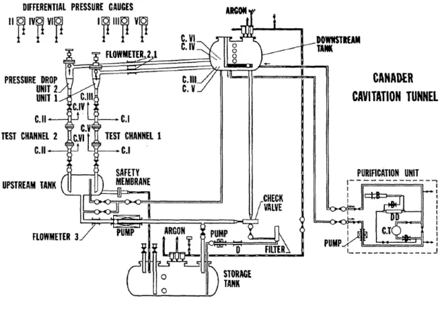
CANADER is a sodium loop whose scheme is shown on figure 1. It has the following boundary operating conditions:
• Temperature: 200◦C to 600◦C • Flow rate: 1 to 7 l/s
• Downstream vessel argon pressure: 1.15 to 5 absolute bars
Flow rate is controlled with an electromagnetic pump and the maximal pressure generated at pump outlet is 8 absolute bars. Minimum downstream vessel argon pressure is 1.15 absolute bars (a bit greater than atmospheric pressure) to limit oxygen entry in the circuit.
Temperature Pressures
545◦C 1.15; 2; 3; 4; 5
450◦C 1.15; 2; 3; 4; 5
350◦C 1.15; 2; 3; 4; 5
250◦C 1.15; 2; 3; 4; 5
Table 1. Sodium test matrix
The experimental test matrix of tempera-ture and pressure conditions tested on the Venturi geometry of CANADER is pre-sented in table 1.
2.2. The Venturi test section geometry The test section is composed of: • a profiled converging tube with a ratio of 27 between inlet tube
section and orifice section • a cylindric orifice
• a conic diverging tube characterized by a half-angle of 7 ◦
2.3. Obtaining cavitation in both facilities
In CANADER facility, cavitation is obtained following this method: • fluid temperature is stabilized in the whole circuit
• gas pressure in downstream vessel is kept constant
• cavitation phenomena is obtained only by acting on flow rate. Starting from a non-cavitating state, flow rate is gradually increased until the onset of cavitation.
The Thoma parameter is used to caracterize the onset of cavitation: σ = Pus− Psat
1/2ρV2 (1)
Figure 2. Venturi Pus is the absolute static pressure measured upstream from the orifice
Psat is the saturation pressure
ρ is the density of the liquid
V is the average velocity through the orifice 3. Modelling
3.1. Description of the CATHARE-3 thermal-hydraulic code
CATHARE-3 is a french two-phase flow modular system code. It is owned and developped since 1979 by CEA and its partners EDF, Framatome and IRSN. See [15] for more details on the code development and validation strategy. One-dimensional (1D), three-dimensional (3D) or point (0D) hydraulic elements can be associated together to represent a whole facility. Thermal and hydraulic submodules (as warming walls, valves, pumps, turbines...etc) can be added to main hydraulic elements to respectively take into account thermal transfer, flow limitation, pressure
rise or pressure drop. Six local and instantaneous balance equations (mass, momentum and enthalpy for each phase) make possible liquid and gas representation for transient calculations. By this way, mechanical and thermal disequilibrium between phases can be represented [16]. Phase averages make necessary the use of physical closure laws in the balance equations system. One closure law concerns the flashing model, which is presented by Bestion in [17]. Cavitation and flashing correspond to the same phenomenon which is a phase change from liquid to vapor when pressure drops locally or in the whole system.
Figure 3. Venturi modelled with CATHARE-3
The flashing model contains two parts:
• a part existing with or without presence of non-condensable (NC) gas and depending on the liquid phase Reynolds and the difference between the liquid temperature Tland the saturation temperature
Tsat(P ).
• a part existing only in the presence of NC gas which tends to facilitate the vapor creation in this case. 3.2. Venturi modelled with CATHARE-3
The converging/diverging tube is modelled using a 1D hydraulic element. The choice of a 1D mesh implies one direction allowed for liquid and gas velocities but two possible ways (positive or negative).
Several meshings have been tested in this study (see paragraph 4.3.1). The meshing presented on figure 3 is composed of 50 meshes.
Two boundary conditions (BC) are defined:
• an inlet BC (down) which imposes fluid velocitiy and temperature (for both liquid and gas even if gas phase is residual) and void fraction as functions of time.
• an outlet BC (up) which imposes static pressure as a function of time. 4. Validation against experimental data
4.1. Available experimental data: Thoma number as a function of Reynolds
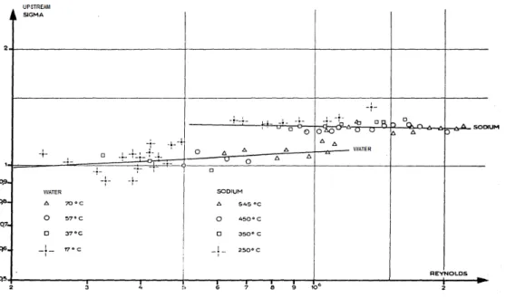
Liquid sodium is an opaque fluid and as a result cavitation cannot be observed with the naked eye. Acoustic methods are used to detect cavitation inception either for small test sections or for a whole SFR. First cavitation detection acoustic method was used in 1957 by Robertson et al [18]. The sigma definition used below corresponds to cavitation inception and the first change of slope in acoustic characteristics [7]. The σ-Re graph on figure 4 was obtained by Courbiere et al in the 1980s by experimenting the Venturi test section in the CANADER loop and in another loop called CALYPSO. Indeed, all test section geometries were also tested with water as working fluid in the CALYPSO loop [3]. In the present paper only sodium tests will be compared to computations. Sodium-water similarity will be studied in the next future.
Figure 4. Thoma number as a function of Reynolds
The aim of the study is to obtain the σ-Re graph presented above by CATHARE-3 calculations.
4.2. CATHARE-3 transient defined to obtain the σ-Re graph
For each pressure-temperature (P-T) couple of conditions, a CATHARE-3 computation is run. As explained in the paragraph 3.2, temperature is imposed as an inlet BC and pressure is imposed as an outlet BC. Both are kept constant during the calculation. Fluid velocity (directly linked to flow rate) is imposed at the inlet BC and gradually increased to obtain cavitation.
The onset of cavitation is detected with a condition on the void fraction reaching a threshold noted αthr at the end of the Venturi throat. When this condition is verified, fluid velocity is
kept constant at its last value corresponding to cavitation inception. Some physical parameters have to be defined to run calculations: • αthr is the void fraction threshold used to detect cavitation inception. • ALIQ is the void fraction imposed at inlet BC.
• XARGON is the fraction of argon NC gas if defined in the computation. • model is the flashing model type used in the computation.
• rugosity is the pipe rugosity used in the computation. Numerical parameters also have to be defined:
• Nmesh is the number of meshes used to model the Venturi test section. All meshes along the Venturi have the same length noted dz.
• DTMAX is the maximal allowed duration of a time step during the calculation (in seconds). In the following paragraph, sensitivity studies will be made by varying these parameters. First, numerical parameters will be tested and a reference set of numerical parameters will be chosen according to mesh and time convergences. Second, physical parameters will be tested and according to physical considerations, a case as representative of the real experiment as possible will be defined.
4.3. Numerical sensitivities
The order of magnitude of meshes used in CATHARE-3 calculations varies in general from 10cm to 1mm. Here, mesh lengths from 2.4cm (25 meshes) to 0.6mm (1000 meshes) will be tested in order to evaluate mesh convergence of calculations.
A standard value of DTMAX used in CATHARE-3 calculations is 1s. Two other values will be tested here: 0.1s and 0.01s in order to evaluate time convergence of calculations.
Finally, the effect of the definition of a NC gas even at a residual value will be studied to ensure that these is no influence on results in this case. Only NC gas rates greater than the residual value must have an effect.
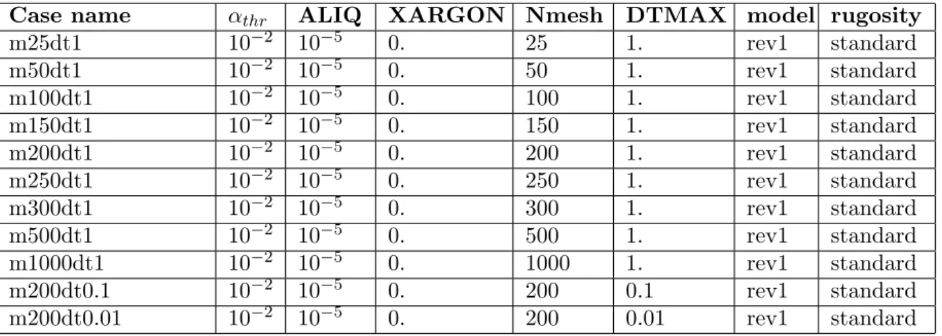
The numerical sensitivity tests matrix is the following:
Case name αthr ALIQ XARGON Nmesh DTMAX model rugosity
m25dt1 10−2 10−5 0. 25 1. rev1 standard m50dt1 10−2 10−5 0. 50 1. rev1 standard m100dt1 10−2 10−5 0. 100 1. rev1 standard m150dt1 10−2 10−5 0. 150 1. rev1 standard m200dt1 10−2 10−5 0. 200 1. rev1 standard m250dt1 10−2 10−5 0. 250 1. rev1 standard m300dt1 10−2 10−5 0. 300 1. rev1 standard m500dt1 10−2 10−5 0. 500 1. rev1 standard m1000dt1 10−2 10−5 0. 1000 1. rev1 standard m200dt0.1 10−2 10−5 0. 200 0.1 rev1 standard m200dt0.01 10−2 10−5 0. 200 0.01 rev1 standard
Table 2. Numerical sensitivities tests matrix
1.037 1.038 1.039 1.04 1.041 1.042 1.043 1.044 1.045 1.046 1.047 -7.5 -7 -6.5 -6 -5.5 -5 -4.5 -4 -3.5 Thoma number (-) log(dz) (-) MESH CONVERGENCE 250°C-4bars case
Figure 5. σ-Re mesh convergence
4.3.1. Mesh convergence To test the mesh convergence, computations using 25, 50, 100, 150, 200, 250, 300, 500 and 1000 meshes are run with other parameters kept constant. Results are available on figure 5 representing the calculated Thoma number for one computation (250◦-4bars case) as a function of the mesh length logarithm. Results are slightly sensitive to the defined mesh. A convergence is obtained by refining the meshing what is satisfactory.
The case using 200 meshes seems to be the good compromise between convergence and CPU time. For this reason, it will be applied for all other following computations.
4.3.2. Time convergence To test the time convergence, computations using a DTMAX value of 1., 0.1 and 0.01 seconds are run for the 200-mesh case. Time convergence is satisfactory according to the results obtained on the global σ-Re graph on figure 6.
A maximal time step duration of 1s seems to be sufficient but more accuracy can be obtained with 0.1s with still reasonable CPU time. For all the following computations, a DTMAX value of 0.1s will be imposed.
4.4. Physical sensitivities
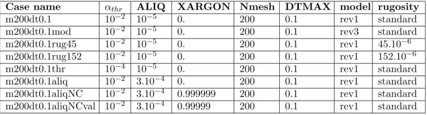
The effect of varying physical parameters is an-alyzed here. Concerning the NC gas presence, from Courbiere [7] it can be considered that the minimal and maximal realistic NC rates respec-tively are 5.10−6 and 3.10−4 cm3Ar/cm3N a.
1.038 1.04 1.042 1.044 1.046 1.048 1.05 1.052 400000 600000 800000 1x10⁶ 1.2x10⁶ 1.4x10⁶ 1.6x10⁶ 1.8x10⁶ Thoma number (-) Reynolds (-) THOMA VS REYNOLDS m200dt1 m200dt0.1 m200dt0.01
Figure 6. σ-Re time convergence
In this study, this volumetric concentration is assumed to correspond to the ALIQ void fraction defined as gas volume/total volume. Indeed, the argon volume is negligible compared to the sodium volume. The minimal value of NC gas presence that can be modelled is the residual one (10−5) which has no effect by definition. Above this residual value, an effect of NC gas presence is expected.
Case name αthr ALIQ XARGON Nmesh DTMAX model rugosity
m200dt0.1 10−2 10−5 0. 200 0.1 rev1 standard
m200dt0.1mod 10−2 10−5 0. 200 0.1 rev3 standard
m200dt0.1rug45 10−2 10−5 0. 200 0.1 rev1 45.10−6
m200dt0.1rug152 10−2 10−5 0. 200 0.1 rev1 152.10−6
m200dt0.1thr 10−4 10−5 0. 200 0.1 rev1 standard
m200dt0.1aliq 10−2 3.10−4 0. 200 0.1 rev1 standard
m200dt0.1aliqNC 10−2 3.10−4 0.999999 200 0.1 rev1 standard
m200dt0.1aliqNCval 10−2 3.10−4 0.99999 200 0.1 rev1 standard
Table 3. Physical sensitivities tests matrix
1.03 1.04 1.05 1.06 1.07 1.08 1.09 1.1 400000 600000 800000 1x10⁶ 1.2x10⁶ 1.4x10⁶ 1.6x10⁶ 1.8x10⁶ Thoma number (-) Reynolds (-) THOMA VS REYNOLDS m200dt0.1 m200dt0.1thr m200dt0.1aliq m200dt0.1aliqNC m200dt0.1aliqNCval
Figure 7. σ-Re physical sensitivities
4.4.1. Sensitivity to the threshold value A sensitivity to the threshold value (αthr =
10−2 or 10−4) has been conducted. Results are not sensitive as shown on figure 7, then, the value of αthr = 10−2 is kept in the
following.
4.4.2. Sensitivity to the void fraction without NC gas A sensitivity to the void fraction value imposed at inlet BC without presence of NC gas (ALIQ = 10−5or 3.10−4 with XARGON=0. in both cases) has been conducted. Results are not sensitive to this parameter without NC gas presence as shown on 7.
4.4.3. Sensitivity to the presence of NC gas A sensitivity to the presence of NC gas imposed at inlet BC (XARGON=0. or XARGON=0.999999 with ALIQ = 3.10−4 in both cases) has been conducted. Results are really sensitive to the NC gas presence as shown on figure 7. NC gas presence is a important parameter to take into account in sodium cavitation studies, what was also identified by Courbiere [7].
4.4.4. Sensitivity to the argon rate value The argon rate value XARGON cannot be set exactly to 1. (100% of gas phase) because residual water vapor phase always exists in CATHARE-3 two-phase computations for numerical reasons. The effect of defining a XARGON value to 0.999999 or 0.99999 is investigated here. Results presented on figure 7 show a little dependence on the value of XARGON. In the following, the value of 0.999999 will be kept.
4.4.5. Sensitivity to the flashing model The default flashing model used in all calculations of this study is the one developped for water applications [17]. But, in the frame of SFR thermalhydraulics studies, the CATHARE development team at CEA proposed to modify two constants of the initial flashing model in order to better represent sodium flow conditions. In this paragraph, results on the prediction of the Thoma number using the modified sodium flashing model will be compared to those using the initial flashing model.
1.038 1.04 1.042 1.044 1.046 1.048 1.05 1.052 400000 600000 800000 1x10⁶ 1.2x10⁶ 1.4x10⁶ 1.6x10⁶ 1.8x10⁶ Thoma number (-) Reynolds (-) THOMA VS REYNOLDS m200dt0.1 m200dt0.1mod
Figure 8. σ-Re model sensitivity
In this cavitation inception study, the modification of the two constants in the flashing model seems not to have a significant influence on results. Currently, there is a lack of data allowing to validate correctly flashing models for sodium applications. Depressurization validation cases need to be experimented and modelled.
4.4.6. Sensitivity to the rugosity Pipe rugosity impacts the pressure drop along the test channel. For this reason, a sensitivity to the rugosity is conducted here. Results using the CATHARE-3 ’RUGO’ option with two absolute rugosities of 45.10−6m (stainless steel) and 152.10−6m (galvanized steel) [19] are compared to results using the classical CATHARE-3 model that corresponds approximately to an absolute rugosity of 1.5.10−6m in this range of Reynolds number. 1.03 1.04 1.05 1.06 1.07 1.08 1.09 1.1 1.11 1.12 1.13 400000 600000 800000 1x10⁶ 1.2x10⁶ 1.4x10⁶ 1.6x10⁶ 1.8x10⁶ Thoma number (-) Reynolds (-) THOMA VS REYNOLDS m200dt0.1 m200dt0.1rug45 m200dt0.1rug152
Figure 9. σ-Re rugosity sensitivity
RUGO is an option of CATHARE-3 developed mainly for high Reynolds applications in the frame of ASTRID gas power conversion system studies [20]. Results presented on figure 9 show a great sensitivity to the pipe rugosity. In the following, the value of 45.10−6m will be kept as it is the most plausible rugosity of the test channel.
4.5. Detailed results of the most representative case
Considering the sensitivity studies conducted and physical considerations mentionned previously, the following representative case is defined:
Case name αthr ALIQ XARGON Nmesh DTMAX model rugosity
representative 10−2 3.10−4 0.999999 200 0.1 rev1 45.10−6
Table 4. The most representative case defined
0.6 0.8 1 1.2 1.4 1.6 1.8 2 200000 400000 600000 800000 1x10⁶ 1.2x10⁶ 1.4x10⁶ 1.6x10⁶ 1.8x10⁶ 2x10⁶ Thoma number (-) Reynolds (-) THOMA VS REYNOLDS experiment representative
Figure 10. σ-Re validation
Comparison of computation results of the most representative case to experimental data is made here. Scale boundaries of initial experimental graph are defined but scaling is linear instead of 2-logarithmic. Difference between the two scalings is small in this case. The experimental line repre-sented in the experimental graph has been reproduced on figure 10. Globally, results are underestimated of approximately 13% compared to experimental data. However, the qualitative trend of the σ-Re curve is respected.
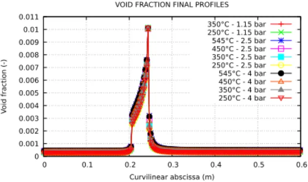
Additionally to the global σ-Re curve, detailed profiles and evolutions of main physical quantities are presented in the following. Evolutions of the inlet BC velocity and the void fraction at the end of the Venturi throat are available on figure 11 and 12 for each P-T couple of conditions. Pressure and void fraction profiles obtained at the end of the transient are presented on figure 13 and 14. 5 10 15 20 25 30 35 0 50 100 150 200 250 300 350 400 450 V elocity (m/s) Time (s) LIQUID VELOCITY EVOLUTION 350°C - 1.15 bar 250°C - 1.15 bar 545°C - 2.5 bar 450°C - 2.5 bar 350°C - 2.5 bar 250°C - 2.5 bar 545°C - 4 bar 450°C - 4 bar 350°C - 4 bar 250°C - 4 bar
Figure 11. Velocity evolutions
0 0.002 0.004 0.006 0.008 0.01 0.012 0 50 100 150 200 250 300 350 400 450 V oid fraction (-) Time (s) VOID FRACTION EVOLUTION 350°C - 1.15 bar 250°C - 1.15 bar 545°C - 2.5 bar 450°C - 2.5 bar 350°C - 2.5 bar 250°C - 2.5 bar 545°C - 4 bar 450°C - 4 bar 350°C - 4 bar 250°C - 4 bar
0 50000 100000 150000 200000 250000 300000 350000 400000 450000 0 0.1 0.2 0.3 0.4 0.5 0.6 P ressur e (P a) Curvilinear abscissa (m) PRESSURE PROFILES 350°C - 1.15 bar 250°C - 1.15 bar 545°C - 2.5 bar 450°C - 2.5 bar 350°C - 2.5 bar 250°C - 2.5 bar 545°C - 4 bar 450°C - 4 bar 350°C - 4 bar 250°C - 4 bar
Figure 13. Pressure profiles
0 0.001 0.002 0.003 0.004 0.005 0.006 0.007 0.008 0.009 0.01 0.011 0 0.1 0.2 0.3 0.4 0.5 0.6 V oid fraction (-) Curvilinear abscissa (m) VOID FRACTION FINAL PROFILES
350°C - 1.15 bar 250°C - 1.15 bar 545°C - 2.5 bar 450°C - 2.5 bar 350°C - 2.5 bar 250°C - 2.5 bar 545°C - 4 bar 450°C - 4 bar 350°C - 4 bar 250°C - 4 bar
Figure 14. Void fraction profiles
0 2 4 6 8 10 12 14 16 0 50 100 150 200 250 300 350 400 450 Thoma number (-) Time (s) THOMA NUMBER EVOLUTION 350°C - 1.15 bar 250°C - 1.15 bar 545°C - 2.5 bar 450°C - 2.5 bar 350°C - 2.5 bar 250°C - 2.5 bar 545°C - 4 bar 450°C - 4 bar 350°C - 4 bar 250°C - 4 bar
Figure 15. Thoma number evolutions
Finally, evolutions of the Thoma number for each P-T couple of conditions as a function of time are presented on figure 15. What can be concluded from all these detailed results is that temperature seems to have a small effect on cavitation inception flow rate instead of pressure that have an important effect.
Conclusions and perspectives
The objective of the present study is to learn about sodium cavitation phenomenon. Indeed, water cavitation occuring in Venturis has been well studied but experiment sodium loops is much more difficult and expensive what explains the lack of available experimental data on the subject.
The CANADER facility operated in the 1980s at CEA Cadarache has been presented in this paper and the tests experimented on the Venturi geometry have been modelled using the CATHARE-3 two-phase flow thermalhydraulic code.
Numerical and physical sensitivity tests have been respectively conducted to better control the obtained results and evaluate the effect of parameters on the predicted Thoma number. The Thoma number corresponding to cavitation inception and its dependence on the Reynolds number has ben studied. Profiles along the test section and evolutions during the transient of quantities of interest have been presented.
The perspective of this work is mainly the study of water-sodium similarity by simulating the CALYPSO tests on the same Venturi test section geometry. That will be done in the next future.
Nomenclature Acronyms
Symbol Description
AST RID Advanced Sodium Technological Reactor for Indus-trial Demonstration
BC Boundary Condition
CAT HARE Code for Analysis of THermalhydraulics during an Accident of Reactor and safety Evaluation
CEA French Alternative Energies and Atomic Energy
Commission
CP U Central Processing Unit
EDF Electricit´e De France
IRSN Institut de Radioprotection et de Sˆuret´e Nucl´eaire
N C Non-Condensable
SF R Sodium Fast Reactor
xD x-dimensional Subscripts l liquid sat saturation thr threshold us upstream Latin letters dz Mesh length P Pressure Re Reynolds number T Temperature V Fluid velocity Greek letters α void fraction ρ density σ Thoma number References
[1] F. G. Hammitt. Cavitation phenomena in liquid metals. La houille blanche, 1:31–36, 1968. [2] R. Bisci and P. Courbiere. Similitude eau sodium en cavitation. IAHR Symposium, 1976.
[3] R. Bisci and P. Courbiere. Analogy of water as compared to sodium in cavitation. Specialists Meeting on Cavitation in Sodium and studies of Analogy with water as compared to sodium, 1976.
[4] P. Courbiere. Sodium cavitation erosion testing. 6th conference on fluid machinery, 1979.
[5] P. Courbiere. Cavitation erosion in sodium flow - sodium cavitation tunnel testing. Symposium on cavitation erosion in fluid systems, 1981.
[6] P. Courbiere J. Defaucheux and P. Garnaud. Acoustic methods in sodium flow for characterising pump cavitation and noise erosion correlations. International symposium on cavitation noise, 1982.
[7] P. Courbiere. An acoustic method for characterizing the onset of cavitation in nozzles and pumps. ASME Symposium on flow induced vibration, 1984.
[8] P. Courbiere. Cavitation erosion in a 400 ◦C sodium flow. ASME Symposium on flow induced vibration, 1984.
[9] T. Ardiansyah M. Takahashi Y. Yoshizawa M. Nakagawa K. Miura and M. Asaba. Acoustic noise and onset of sodium cavitation in venturi. Sixth Japan-Korea Symposium on Nuclear Thermal Hydraulics and Safety, 2008.
[10] T. Ardiansyah M. Takahashi M. Nakagawa. Effect of argon gas injection on acoustics noise and onset of sodium cavitation in venturi. NURETH-13, 2009.
[11] T. Ardiansyah M. Takahashi Y. Yoshizawa M. Nakagawa M. Asaba and K. Miura. Numerical simulation of cavitation for comparison of sodium and water flows. Proceedings of the 18th International Conference on Nuclear Engineering ICONE18, 2010.
[12] T. Ardiansyah M. Takahashi Y. Yoshizawa M. Nakagawa K. Miura and M. Asaba. The onset of cavitation and the acoustic noise characteristics of sodium flow in a venturi. Journal of Power and Energy Systems, 5:33–44, 2011.
[13] T. Ardiansyah M. Takahashi M. Asaba and K. Miura. Cavitation damage in flowing liquid sodium using venturi test section. Journal of Power and Energy Systems, 5:77–85, 2011.
[14] F. Varaine et al. Pre-conceptual design of astrid core. ICAPP-12, 2012.
[15] F. Barre and M. Bernard. The CATHARE code strategy and assessment. Nuclear Engineering and Design, 124:257–284, 1990.
[16] B. Faydide and J.C. Rousseau. Two-phase flow modeling with thermal and mechanical non equilibrium. European Two Phase Flow Group Meeting, 1980.
[17] D. Bestion. The physical closure laws in the CATHARE code. Nuclear Engineering and Design, 124:229–245, 1990.
[18] J. M. Robertson J. H. McGinley J. W. Holl. On several laws of cavitation scaling. La houille blanche, 4:540–554, 1957.
[19] Hydraulic Institute. Hydraulic Institute Engineering Data Book. 2nd Edition, 1990.
[20] G. Mauger F. Bentivoglio and N. Tauveron. Description of an improved turbomachinery model to be developed in the CATHARE-3 code for ASTRID power conversion system application. NURETH-16, 2015.