A comparison of discrete and flow-based models for air traffic flow management

A comparison of discrete and flow-based models

for air traffic flow management

by

Thi Vu Phu

Submitted to the School of Engineering

in partial fulfillment of the requirements for the degree of

Master of Science in Computation for Design and Optimization

at the

MASSACHUSETTS INSTITUTE OF TECHNOLOGY

September 2008

MASSAC OF

SE

@ Massachusetts Institute of Technology 2008. All rights reserved.

P

A uthor ...

Certified by ...

...

Assistant Professor of Aeronautics and

School of Engineering

August 2, 2008

.. . . .. ..

Hamsa Balakrishnan

Astronautics and Engineering

Systems

Thesis Supervisor

Accepted by..

...

_{... . ....}

_u

_~•.

_{- ...}

... Jaime Peraire

Professor of Aeronautics and Astronautics

Codirector, Computation for Design and Optimization

ARCHIVE

HLUSETTS INSTITUTE TECHNOLOGY

:P

0 5 2008

A comparison of discrete and flow-based models for air

traffic flow management

by

Thi Vu Phu

Submitted to the School of Engineering on August 2, 2008, in partial fulfillment of the

requirements for the degree of

Master of Science in Computation for Design and Optimization

Abstract

The steady increase of congestion in air traffic networks has resulted in significant economic losses and potential safety issues in the air transportation. A potential way to reduce congestion is to adopt efficient air traffic management policies, such as, optimally scheduling and routing air traffic throughout the network. In recent years, several models have been proposed to predict and manage air traffic. This thesis focuses on the comparison of two such approaches to air traffic flow management: (i) a discrete Mixed Integer Program model, and (ii) a continuous flow-based model. The continuous model is applied in a multi-commodity setting to take into account the origins and destinations of the aircraft. Sequential quadratic programming is used to optimize the continuous model. A comparison of the performance of the two models based on a set of large scale test cases is provided. Preliminary results suggest that the linear programming relaxation of the discrete model provides results similar to the continuous flow-based model for high volumes of air traffic.

Thesis Supervisor: Hamsa Balakrishnan

Acknowledgments

First and foremost, I would like to thank my advisor, Professor Hamsa Balakrish-nan for initiating this research project and for her continuous guidance and support. Whenever I had problems with my research, she would work patiently with me to find the answers to difficult problems. Even when she was busy with her schedule oversea, she still wanted to talk to me over the phone to know my progress and answer my

questions. I was so lucky to work with such a thoughtful and dedicated advisor.

My time in MIT was a wonderful experience and I have learnt so much in a rel-atively short period of time. I would like to thank Professor Gilbert Strang for the inspiring and exciting lectures in numerical analysis, he was always patient to answer my questions and motivated my study. I would like to thank Professor David Dar-mofal, Professor Jacob White, Professor Anthony Patera, Professor Luca Daniel and Professor Jaime Peraire for introducing me to the field of numerical partial differential equations. I would like to thank Professor Thomas Magnanti and Dr Brian Anthony for introducing me to the various methods in system optimization which were really helpful in my research.

Special thanks to my friends from the SMA CE Program. Although we have just known each other for a short time, we have shared so much joy and overcome all the challenges in this rigorous program. My life in Boston would not have been so lively and joyful without all of you. I also would like to thank Michael Lim, Jocelyn Sales and John Desforge from SMA; Laura Koller from CDO Program for their excellent support.

This research was fully funded by the Singapore MIT Alliance graduate fellow-ship. In addition, professor Balakrishnan provided me with the latest software and computing tools for the computational experiments.

Last but not least, I am forever indebted to my family for their unconditional love and support. My parents, Don Hau Phu and Thu Ha Truong; and my sister, Nguyet Minh Phu, have always been my pillars of support throughout the years. The long distance calls, emails and messages from them are my greatest encouragements and they have made me never feel lonely when living far away from home.

Contents

1 Introduction 13

1.1 Overview of air traffic management . . . . 13

1.2 Literature Review ... ... .... .. 15

1.2.1 Multicommodity Eulerian-Lagrangian Large-capacity Cell

Tran-mission Model for Enroute Traffic . ... 15

1.2.2 The Multi-Airport Ground Holding Model . . . . 17

2 Discrete Enroute Air Traffic Flow Management Model 21

2.1 Definitions and notations . . . . .. .. . . . 21

2.1.1 Discrete model formulation ... .. 22

2.1.2 A variation of the Discrete Enroute Air Traffic Flow

Manage-m ent M odel . . . 24

2.2 LP Relaxation ... ... ... ... ... ... 26

3 Continuous flow-based network model of air traffic flow 29

3.1 Single commodity air traffic model in a link . . . . 29

3.2 Single commodity network model . . . . 31

3.3 Multi-commodity network model of traffic flow . . ... . . . . 33

4 Optimal control of air traffic flows 37

4.1 The optimal control problem ... .. 37

4.2 Formulating the Finite Difference Scheme . . . . .. . . . . 38

4.2.2 Steepest Descent method ... .. 40

4.2.3 Newton Method ... 41

4.3 Sequential Quadratic Approximation Method . ... 43

4.3.1 Summary of the algorithms . ... 46

4.3.2 Sequential Quadratic Programming Algorithm ... . 47

5 Computational Results 49 5.1 The Test Data ... .. ... ... ... .. ... 49

5.2 The results . . . .. . 51

5.2.1 C ase I . . . 51

5.2.2 C ase II . . . 60

5.3 Summary of the difference in two models . ... 69

List of Figures

3-1 Conservation of mass in control volume V ... 30

3-3 Flow-splitting problem ... 34

3-4 A simple multi-commodity network ... ... 34

5-1 Multi-commodity network ... 50

5-2 Arrival record at airport Al for Continuous model ... 53

5-3 Arrival record at airport Al for Discrete (R) model ... 53

5-4 Arrival record at airport Al for Discrete (I) model ... 53

5-5 Arrival record at airport A2 for Continuous model ... 53

5-6 Arrival record at airport A2 for Discrete (R) model ... 53

5-7 Arrival record at airport A2 for Discrete (I) model ... 53

5-8 Flow split coefficients for commodity 1 ... ... 54

5-9 Flow split coefficients for commodity 2 ... 54

5-10 Flow split coefficients for commodity 3 ... ... 54

5-11 Flow split coefficients for commodity 4 ... ... 54

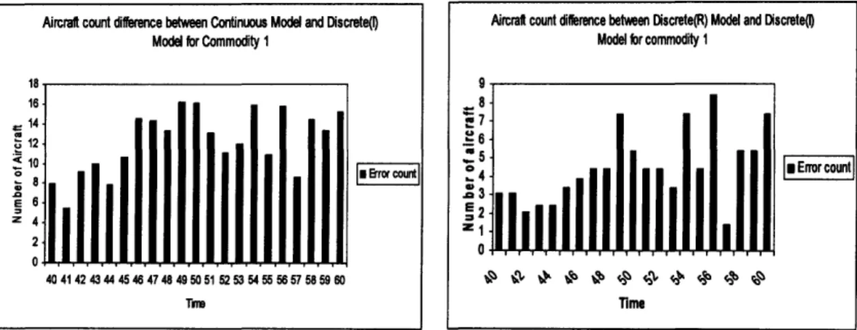
5-12 Continuous and Discrete (I) (Commodity 1) ... 55

5-13 Discrete (R) and Discrete (I) (Commodity 1) ... 55

5-14 Continuous and Discrete (R) (Commodity 1) ... 55

5-15 Continuous and Discrete (I) (Commodity 2) ... 56

5-16 Discrete (R) and Discrete (I) (Commodity 2) ... 56

5-17 Continuous and Discrete (R) (Commodity 2) ... 56

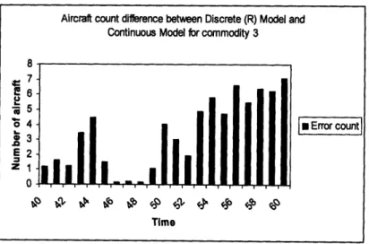
5-18 Continuous and Discrete (I) (Commodity 3) ... 57

5-19 Discrete (R) and Discrete (I) (Commodity 3) ... 57

5-20 Continuous and Discrete (R) (Commodity 3) ... 58

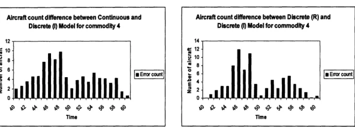
5-22 Discrete (R) and Discrete (I) (Commodity 4) ...

5-23 Continuous and Discrete (R) (Commodity 4) ...

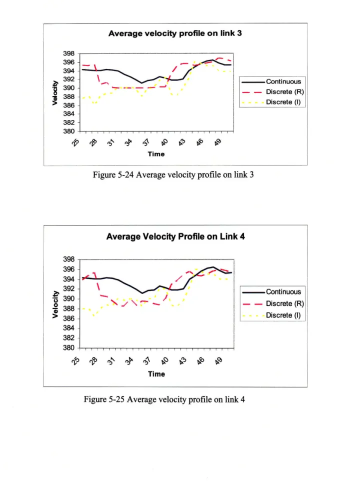
5-24 Average velocity profile on link 3 ... ...

5-25 Average velocity profile on link 4 ... ...

5-26 Arrival record at airport Al for Continuous model ... 5-27 Arrival record at airport Al for Discrete (R) model ... 5-28 Arrival record at airport Al for Discrete (I) model ... 5-29 Arrival record at airport A2 for Continuous model ... 5-30 Arrival record at airport A2 for Discrete (R) model ... 5-31 Arrival record at airport A2 for Discrete (I) model ... 5-32 Flow split coefficients for commodity 1 ... 5-33 Flow split coefficients for commodity 2 ... 5-34 Flow split coefficients for commodity 3 ... 5-35 Flow split coefficients for commodity 4 ... 5-36 Continuous and Discrete (I) (Commodity 1) ... 5-37 Discrete (R) and Discrete (I) (Commodity 1) ... 5-38 Continuous and Discrete (R) (Commodity 1)

5-39 Continuous and Discrete (I) (Commodity 2) 5-40 Discrete (R) and Discrete (I) (Commodity 2) 5-41 Continuous and Discrete (R) (Commodity 2) 5-42 Continuous and Discrete (I) (Commodity 3) 5-43 Discrete (R) and Discrete (I) (Commodity 3) 5-44 Continuous and Discrete (R) (Commodity 3) 5-45 Continuous and Discrete (I) (Commodity 4) 5-46 Discrete (R) and Discrete (I) (Commodity 4) 5-47 Continuous and Discrete (R) (Commodity 4)

5-48 Average velocity profile on link 3 ...

5-49 Average velocity profile on link 4 ... ..

59 59 60 60 62 62 62 62 62 62 63 63 63 64 65 ... ... °°...o°.o... ... o°... ... °°...°...° ... ... o°°... ... •...°°.. ... ... °°...°...° .... ... °...o...° ... °...°°°...°...° ..o ... ... ... ... °° °o °° ...o... .. '" "" " " "" " '" " .. " " "" " " .. " " " " ' " " " .. " " " " " " "" '"" " .. " '" ' " '" '" .. " " " " " " '" " "" .. " " " " "'" " " " "

List of Tables

5.1 Comparison of arrival records at destination airport Al (Case I) . . . 51

5.2 Comparison of arrival records at destination airport A2 (Case I) . . . 52

5.3 Comparison of arrival records at destination airport Al (Case II) . 60

5.4 Comparison of arrival records at destination airport A2 (Case II) . 61

Chapter 1

Introduction

1.1

Overview of air traffic management

Air transportation is a multi-billion dollar industry and one of the fastest growing sectors. In 2006, there were 21 million flights worldwide and more than 31,000 flights per day in the US alone. The demand for air transportation has grown steadily in the past few decades and is expected to reach 2-3 times current levels by the year

2025 [15]. The rapid growth of air traffic has become a critical issue as most elements of the National Airspace System (NAS) are subject to capacity constraints. Conges-tion occurs when there is an imbalance between demand and capacity constraints. Congestion in the NAS not only causes flights delays but also poses many potential safety issues. It has been estimated that failure to address the impact of air traffic congestion would cost US consumers approximately $20 billion per year by 2025 [15]. The issue of congestion in air transportation is a complicated problem which includes, but is not limited to, infrastructure design and services, air traffic manage-ment, and airport operations. Of these, air traffic managemanage-ment, which optimizes the throughput while maintaining the number of aircraft at safe levels, is an important factor and has been the focus of extensive research. Air traffic management (ATM) is the dynamic, integrated management of air traffic and airspace in safe, economical and efficient ways. One of the key elements in ATM is the control of air traffic in the enroute airspace, which typically involves ensuring that the number of aircraft

in regions of the airspace to be below predetermined thresholds. This ensures safety of the flights and eases the workload of air traffic controllers. Although this task is similar to the control of highway or road traffic, it is more challenging due to the complicated nature of the air transportation system.

The Federal Aviation Administration (FAA) has been using ground-holding poli-cies to reduce delay costs. This policy is implemented in a nationwide program called the Ground Delay Program (GDP). It is operated on the assumption that in conges-tion situaconges-tions, if an aircraft departs on time, then it will incur enroute congesconges-tion and airborne delays. Airborne delays are harder to handle and more expensive in terms of fuel cost than delaying the aircraft on the ground. Hence, one of the objec-tives of the ground delay program is to transfer airborne delay costs to ground delay costs. Currently, the GDP is usually innitiated when there are closed runways, se-vere weather (i.e. low visibility, thuderstorms, heavy snow),and overloaded airports. The FAA uses a computerized procedure to choose the ground-holds on a first-come, first-served basis. Over the years, several models have been developed to optimize the procedure and to enhance the effectiveness of traffic flow management in the US airspace, where congestion has been an increasingly important problem.

Discrete models which take into account individual trajectories of aircraft and provide optimal schedules were introduced in the 1980s and 1990s in the work of Vranas et al. [23], Bertsimas et al. [5] and others. These models often result in large Mixed Integer programs. Techniques such as branch-and-bound, branch-and-cut and columns generations were used in solving such problems and provide good results in a number of test cases; however, large memory usage is a problem with these discrete models. Recently, control volume based models inspired by hydrodynamic theory for highway traffic flow (in particular the work of Lighthill Whitham and Richard (LWR) [13], [17]) have been introduced in several papers such as those Sun et al. [21], and Bayen et al. [4]. These models rely on conservation equations to simulate and optimize the flow of air traffic. One advantage of these models is that the size of the problem only depends on the physical structure of the networks and not on the number of flights; indeed, the models are more accurate with larger numbers

of flights. There are also some hybrid models which are control volume based but take into account some trajectory information such as the Origin-Destination (OD) information of flights. In the next section, we review some of the models in literature that are relevant to our work.

1.2

Literature Review

1.2.1

Multicommodity Eulerian-Lagrangian Large-capacity Cell

Tranmission Model for Enroute Traffic

The single commodity Large Cell Tranmission Model

The Large Cell Transmission Model (CTM(L)) was proposed by Daganzo et al. in [21], [9]. This model uses a graph-theoretic representation of traffic flow, in which each link of the network is modeled by a directional edge. Each edge consists of many cells and the number of cells in a link is given by the number of steps of expected travel time of the aircraft, which are assumed to fly at an average aggregate speed. For example, if it takes 10 time-steps for the aircraft to fly across a link then this link would consist of 10 cells. The choice of the time discretization (number of time steps) of a link is arbitrary and is user-specified. At each link, only aircraft above a certain altitude are taken into account. The behavior of aircraft flow on a link will then be modeled by the linear dynamical system:

x (k + 1) = A xi(k) + B{ fi(k) + BYui(k) (1.1)

y(k) = Cixi(k), (1.2)

where

xi(k) = [xm' (k),..., xL (k)]T: the state vector which represents the numeber of aircrafts

fi(k): the forcing input which is the number of flights entering link i during a unit

time interval from k to k + 1.

ui(k): an mi x 1 vector, representing holding pattern control, which is the number of flights which are held in link i at time interval k.

y(k): the aircraft count at time interval k.

Ci: the output vector, the nonzero elements of the vector Ca (equal to one) correspond

to the cells in the links.

Ai: a mi x mi nilpotent matrix with 1's on its super-diagonal, i.e. [ U 1 0 ... ... O 0 0 1 0 ... O0 0 0 0 1 ... O0 0 0 0 0 ... 1 on _{~ v v} n _v u nov I

Bif = [0, ... , 0, 1]T: the forcing vector with mi elements.

Bi": the mi x mi holding pattern matrix, in which all non-zero elements are 1 on the diagonal and -1 on the super-diagonal.

The one link level model can easily be extended to the sector level model. Suppose a sector consists of n links, the sector level CTM(L) model can be described as:

x(k + 1) = Ax(k) + B f (k) + B"u(k) (1.3)

y(k) = Cx(k),

(1.4)

where x(k) = [xn(k);...;xl(k)]T denotes the state; f(k) = [fn(k);...; fi(k)]T is the forcing input; u(k) = [u,(k); ...; ul(k)]T is the holding patterns. The matrix A =

diag(A, ...., A1) is a block diagonal matrix, with Ai being the matrix for the link i as

in equation (1.1). Similarly, the matrix Bf, B" are also block diagonal matrices with

the diagonal blocks corresponding to the respective matrices in the link level model.

The control inputs for this model are given by the holding patterns which are represented by u, the forcing input f, and the spacing of the aircrafts as represented

by xi.

Multicommodity CTM(L) Model

In the CTM(L) model, air traffic is aggregated and the orgin-destination information of flights are not taken into account. This will result in the traffic flow split problem since according to the model in which flights are not guaranteed to arrive at the original destinations. We will discuss this problem in more details in chapter 3. In the multicommodity CTM(L) model, this problem is resolved by incorporating knowledge of the destinations of the aircrafts (which are available in the form of filed flight plans) into the model. Flights are clustred based on their origin-destination (OD) node pairs in the network. Each pair corresponds to a path consisting of links between these nodes. This results in a multicommodity network flow structure. We note that this multicommodity framework can also be extended to other models and in this thesis we will modify the PDE model in the same manner that take into acount the OD pairs.

1.2.2

The Multi-Airport Ground Holding Model

Ground-holding has been in use for several years, especially in the Ground Delay Program (GDP) where expensive airborne delay cost is transfered into ground delay cost. The FAA operates an Air Traffic Control System Command Center (ATCSCC) in Washington, D.C., where holding decisions are made by experiened air traffic controllers equipped with extensive information-gathering capabilities. In the early 1990s, the holding patterns were mostly decided by expert air traffic controllers with-out relying on optimization models to develop flow management and ground-holding strategies in a system wide basis. In 1993, Menon et al. introduced a multi-airport

ground holding model [21] which used a mathematical programming approach to solve the ground-holding problem in a general setting. This model was extended to the dis-crete Enroute air traffic flow management model by Bertsimas et al. in [5] which will be discussed in the next chapter [4].

Notations and definitions We consider:

IC = {1, ..., K}: a set of airports,

T = _{{1, ..., T}: an ordered set of time periods,}

F = {1,..., F}: a set of flights,

k E IC: the airport from which flight f is scheduled to depart,

fk E IC: the airport at which flight f is scheduled to arrive,

df E T: the scheduled departure time of flight f,

rf E T: the scheduled arrival time of flight f,

c'(.): the ground delay cost function of f (in time period t), c'(.): the airborne delay cost function of f (in time period t),

Dk(t): departure capacity of airport k at time period t, Rk(t): arrival capacity of airport k at time period t, F' C F: a set of flights that are continued.

The decision variables are defined as follows:

gf, f E F: the number of time periods that flight f is held on the ground before being

allowed to take-off,

af, f E F: the number of time periods that flight f is is further held in the air before

being allowed to land.

By introducing the assignment variable uft, where uft is equal to one if flight f is

vft, where vft is equal to one if flight f finally is assigned to land at time period t

and zero otherwise, the above decision variables can be rewritten as:

9 = Z tuft - d, f E F; (1.5)

tETP"

a1 = : tvjt - rf -i -F. , f E (1.6)

where

Tfd: set of time periods to which flight

f

fT7: set of time periods to which flight f may be assigned to land.

The Multi-Airport Ground Holding Model (MAGHP)

The model is then formulated as follows:

F min Z(cfg

+

Suft

In the above formulation, the cost function represents the total delay cost (both airborne and ground delays) of all the flights in the system. Constraints (1.8) and

(1.9) represent the departure and arrival capacity constraints, respectively. Constraint (1.10) ensures that exactly one assigment variable uft is equal to one, similarly for constraint (1.11). Constraint (1.12) ensures that any excessive delay of flight f' is transfered to its next flight (connection flight) f, where sf is the slack time which is the time needed before flight f' can connect to the next flight f (e.g. time for refueling, maintainance of aircraft).

The MAGHP model was modified and improved by Bertsimas et al. in [5] to take into account the air sectors constraints instead of just the airports' capacity constraints. A change in the definition of the assignment variables in [5] has also been shown to improve the effectiveness of the model. We will discuss this model [5] in the subsequent chapters.

Chapter 2

Discrete Enroute Air Traffic Flow

Management Model

In this chapter, we discuss the formulation of the enroute air traffic flow management model in [4] which will be used to compare with the continuous flow-based model in [5]. We know that this model is an extension of the multiple-airport ground holding (MAGHP) model [23] that has been discussed in the previous chapter. We remove the connection flights constraints in the original model and change the objective function to maximizing of the throughput of aircrafts in selected airports. The airport capacity constraints are also removed as we will treat airports and sectors as similar entities.

2.1

Definitions and notations

Consider a set of flights F = {1, ..., F} , a set of air sectors J = {1, ..., J} , a set of airports K = {1, ..., K} , and a set of time periods T = {1, ..., T}.

Here F is the set of all flights of interest, i.e. all flights that leave an airport

and enter another airport within K1C. We note that our network is closed, that is, all

flights whose origins and destinations lie outside the network are neglected. For ease

of notation, we refer to a sector j as either an airport or an air sector and redefine J

We consider some additional notation:

* N1: number of sectors in the path of flight f * P(f, i): the ith sector in the path of flight f * Pf = (P(f, i) : 1 < i < Nf: the path of flight f * Sj(t): capacity of sector j at time t

* lfj: number of time periods that flight f must spend in sector j

* T]: set of time periods for flight f to start its path passing through sector j * T]: the earliest time that flight f can be in sector j

* T]: the latest time that flight f can be in sector j

If negative delays are not allowed, we note that:

•> "t + j,

Vf E :F,j' = P(f,i),j = P(f,i + 1), i < N.

2.1.1

Discrete model formulation

We define a binary variable jft(f E F,

j

arrives at sector j by time period t, and 0 otherwise. This definition using by and not at is critical in this model. It has been shown in [1] that the LP relaxation of the Discrete Enroute Air Traffic Flow Management Model using by is tighter than the LP relaxation of that model using at in the definition of the variables . Recall that

we have also defined for each flight f a path P1 which is the list of sectors that flight

f must pass through, so the variables W.jet will only be defined for those elements j

time periods within the feasible set T/. Therefore, whenever a variable wu3 is used in the formulation, it corresponds to a feasible (f, j, t) combination. Furthermore, since

flight f must arrive at sector j by the latest time , w = 1. There are many

potential objectives in traffic flow management, including minimizing the total delay time of flights, minimizing the cost due delays and limiting the workload of air traffic controllers. In this thesis, we consider the objective of maximizing the throughput of air traffic at a selection of destination airports. The objective of the optimization problem is formulated as follows:

max _(w

_f

_,

₎₎

(2.1)

teT,k=P(f,Nf)

tETf ,k=P(f ,Nf )

where the airports k

e

the throughput.

We now present the objective function together with the complete formulation of the model: min

Z

_(ft

_(2.2)

Vf E F, t E T, j = P(f,

.,

Wft

E

{0,1}.

The first constraint ensures that the number of flights in a sector at any time period will not exceed the capacity of that sector. The second constraint, which can be referred as "connectivity in time" constraint, ensures that if a flight has arrived at

wIt

-

Wt-1

>

0,

(2.5)

sector j by time t, then w j has to have a value of 1 for all later time periods t' > t. The third constraint represents connectivity between sectors. It stipulates that if a flight arrives at sector j' by time t + Ifj then it must have arrived at sector j by time

t where

j

j'

f.

2.1.2

A variation of the Discrete Enroute Air Traffic Flow

Management Model

In the previous formulation, each flight had only one path and when congestion oc-curred in the network, flights were held in their current sectors until congestion was clear. An alternative way to manage traffic is to allow the flights to take alternative routes to avoid congestion. In practice, extreme weather conditions often force the capacities of some sectors in the NAS to drop to levels at which no additional flights are allowed to enter these sectors for safety reason. The current formulation will provide a suboptimal solution since most flights will be held in the current positions if any sectors common to the flight paths have a significant drop in capacity. In this section, we extend this model to accomodate rerouting decisions.

We first define Qf to be the set of possible routes of flight f. We note that in

the previous formulation Qf _ Pf . In order to capture the rerouting, we extend the

variables in the following manner: wf' = 1 if flight f arrives at sector j by time t

and wf, = 0 otherwise. We note that the variables in the previous formulation can now be written as:

f=

ft

(2.7)

We consider some additional notation in the modified model:

* Rf: number of possible routes of flight f

*

Q(f,

o Qf = (Q(f, r, i) : 1 < i < Nf, r < Rf): the path of flight f

* If,j,r: number of time periods that flight f must spend in sector j along route r.

The new model can now be expressed as follows:

max E Q (wr wk,r1)

(2.8)

S(w

wg+ _f,t+li,j,r - wr < 0O _f,t Vf E F: Vr E Qf,j= Q(f,r,i),j' = Q(f,r,i + 1),i

W, 32 > 0 Vf E F: Vr E Q2,j = Q(f,r,i),t E T, wC,t E {0,1} _{Vf E F: Vr E Qf,j= Q(f,r,i),t E Tf.}

< Nf,

The objective function now represents the maximum number of flights from all possible routes that arrive at the destination airports. The first constraint ensures that the total number of flights from all routes which may arrive at a sector j at time

the connectivity between sectors is satisfied and the third constraint ensures that the connectivity in time is satisfied along all routes in the network.

2.2

LP Relaxation

Because the Mixed Integer formulation of the Discrete Enroute Air Traffic Flow Man-agement Model cannot be solved in polynomial time [11], we consider the LP relax-ation of the problem which can be solved faster. The LP Relaxrelax-ation is:

max

Z1Wf:

,(wf,

0w'r)

•

Sj(t)

,t+i, r • - w 0 Vf E F: Vr E Qf, j = Q(f,r,i),j' = Q(f,r,i + 1), i

w, - wt_₁ 20 >_r Vf E F: Vr E Q, j = Q(f, r, i), t E T,) 0 < uw < 1 Vf E : Vr E Qf, j = Q(f, r, i), tE TY]. < Nf,

(2.15)

(2.16)

We note that on one hand, the LP relaxation is guaranteed to be solved de-terministically in polynomial time [11], on the other hand the solution is no longer guaranteed to be integers which mean we cannot expect an exact routing of individual

flights based on the result of the LP relaxation. Our conjecture is that the solution of the LP relaxation is similar to the output of the continuous flow-based model which is not based on individual flight trajectory. Therefore, our comparison will focus on the LP relaxation of the discrete model and the continuous flow-based model. In subsequent chapters, we will refer the Discrete Model as Discrete (I) model and the LP Relaxation of the Discrete Model as Discrete (R) model.

Chapter 3

Continuous flow-based network

model of air traffic flow

The flow-based approach in network modeling for air traffic is strongly inspired by hydrodynamic theory for highway traffic (in particular by the work of Lighthill, Whitham and Richards [13], [17]. This framework is sometimes referred to as the LWR theory, and was introduced in various models for air traffic flow management

[4], [21], [19]. In this chapter, we examine a flow-based model, modified from the Eu-lerian network model proposed by Bayen et al. in [4]. This model relies on the LWR partial differential equations (PDE) and the theory of conservation of mass. We mod-ify this model to take into account the origin-destinations (OD) information of flights and avoid the flow splitting problem. In the next sections, a detailed formulation of the model is presented.

3.1

Single commodity air traffic model in a link

We represent a portion of the airspace, for example a jet way, by a segment of a link [0, L] where L is the length of the link. We let n(x, t) be the number of aircraft at position x on the link at time t and let v(x, t) be the aggregated mean velocity of the traffic flow at the x on the link at time t. The density of aircraft at position x at time

On(x, t)

p(, t) = (, t)

(3.1)

Conservation of mass is applied to the control volume of aircraft on the link from

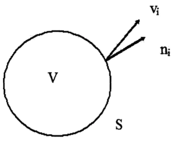
x to x + Ax. We first consider a general case of an arbitrary control volume V, as

shown in Figure 3-1.

vi

ni

Figure 3-1: Conservation of mass in a control volume V

Suppose we have a fluid with local density p(x, t) and local velocity v(x, t). Con-sider a control volume V with boundary S. The mass in this control volume is:

M = pdV,

The rate of change of this mass is

Ot at pdJ V = dV,

The changes result from the mass flow through the boundary surface:

OM

amt = s pvinidS,

30

Using the Divergence theorem, we have

I

atdV

+ I a(pvi)dV

= 0,

(3.3)

S(L

Since V is arbitrary, we have the general form of the conservation of mass of traffic flow:

&p 8

S+ a (pvi) = o.

(3.5)

at axi

Applying equation (3.5) to our aircraft control volume on the link from x to x+Ax and taking into acount the initial and boundary conditions of the flow, we have the governing partial differential equations of the aircraft evolution on a single link:

I

o

at aOx

p(x, 0)

=

Po0()

(3.6)

p(O, t)v(O, t) = qi"(t)

In equation (3.6), po(x) is the initial density of aircrafts on the link (at time 0), and qin(t) represents the inflow of aircraft at the entrance of the link at time t. For simplicity, we can assume that velocity only varies with time, and so the above equation can be written as:

I

_{+ v(t)aP(,t) = 0}

p(x, 0) = po(s) (3.7)

p(O, t)v(t) = qin(t)

3.2

Single commodity network model

Equations (3.6) and (3.7) describe the evolution of aircraft on a single portion of the airspace or a link; we now extend it to a network model. We consider a junction with m incoming links and n outgoing links; each link i is represented by an interval

junctions can depict any network and thus can describe the entire national airspace system (NAS) or any portion of the airspace. Figure 3-2 shows a junction with m incoming links and n outgoing links.

Figure 3-2: A junction with m incoming links and n outgoing links.

In Figure 3-2, the links (m+ 1) to (m + n) are outgoing links where traffic diverges and the link 1 to m are incoming links where traffic converges. Let aij (t)(0 < 1aj < 1) be the portion of aircraft from link i that goes to link j at time t, we have the following relationship:

Pi(0, t) = 1 flijp(L, t)vi(t)

v~(t)

(3.8)

where

=,j(t)=

1.

(3.9)

i=1

The governing equations of the single commodity network model of air traffic flow can now be represented by:

pi(,t)

+ (t)

= o0

Pi(x,

0)

=

po,i(x)

pi(O, t)vi(t) = qi (t)

Pi(O, t) -'- = l3ij (t)pi(Li,t)vi(Li)_vi(o,t)

z:

* 2 is the set of all links in the network

* In(j) is the set of all links that merge to link j

* O is the set of all links that other links merge into it

* po,i is the initial density on the link i at time 0

* qi (t) is the inflow of link i at time t.

3.3

Multi-commodity network model of traffic flow

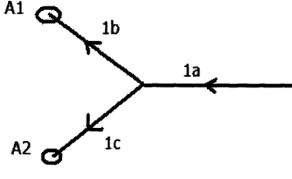
In the previous work of Bayen at al. [4], [18], the information of origins and destina-tions of flights were not taken into account. Therefore, the solution provided by the model used to compute the optimal control strategy may not be feasible in practice since flights are not guaranteed to be routed to the right destinations. To illustrate this problem, we consider the following simple example:

A4

Al

A2

Figure 3-3: Flow-splitting problem

In Figure 3-3, the link (la) diverges into two links (lb) and (ic) with 2 destination airports Al and A2 at the end of the two links repestively. There are 40% of flights in link (la) that have the final destination at airport Al and 60% of flights in link (la) that have the final destination at airport A2. Suppose that capacity of link (Ic) is higher than capacity of link (lb) and the objective is to maximize the throughput at both Al and A2. By not taking into account the Origin-Destination (OD) infor-mation of the flights, a solution may end up sending 70% of flights in (la) to A2 and

30% of flights to Al. This results in a large portion of the flights being sent to the wrong destinations since only 40% of them have Al as their final destination.

We note that the model in [4] may provide a feasible solution if there is a single sink, i.e. only one destination airport. This is not applicable in a general air traffic network. In order to overcome this problem, we add another layer of complexity to the current single commodity model of the air traffic flow problem. Flights are grouped based on the origin-destination pairs (OD pairs). The OD information can be obtained from the flight plans which are available before the actual departure times. The flights between an OD pair are considered as a type of "commodity". Figure 3-4 shows a simple multi-commodity network with four different types of commodities.

- £

I ~ sc

Figure 3-4: A simple multi-commodity network

The continuous flow-based model is reformulated as follows:

apý(x,

t)

ap

(x,

t)

p(0, t) =

vi(0)

p

(x,

0)

= p,o(x),

_{vj (t)}

Vi

E

I, Vk E

I()),

(3.12)

(3.15)

C

where

* IC(i): The set of all "commodities" travelling through link i E I

* p4 represents the density of commodity k on link i

* p is the portion of flow of commodity k that travel from link i to link j

Equation (3.11) describes the conservation of mass property for each type of com-modity on a link. We note that the conservation of mass is satisfied on every link as it is satisfied for each commodity flowing through that link. Equation (3.12) and (3.14) are the boundary conditions for the incoming and outgoing links. Equation (3.13) is the initial condition of the density on the links, and Equation (3.15) ensures that the model is realistic; every the aircraft has to leave on an outgoing link and enter on an incoming link.

Chapter 4

Optimal control of air traffic flows

4.1

The optimal control problem

In this chapter, we study the continous flow-based approach for the optimal con-trol of air traffic in the network. Similar to the discrete case, we try to maximize the throughput of aircrafts at some destination airports. We consider the objective function:

max

H((t),

=

E

ZE

f

t)vi(t) dxdt

(4.1)

The constraints are:

oa

+ v 4(t) .

_{p(0o, t)}

_a

=

= o,

t)

vi (0)

pi(x,

) =

p,

o(),

(0, t)

(0)

Vi

Sjf(t)

=

1, Vi

E 1, Vje J, Vk E

K(i).

(4.2)

(4.4)

(4.5)

(4.6)

4.2

Formulating the Finite Difference Scheme

It is generally not possible to solve system (4.1) - (4.6) analytically when v depends

on time [4]. In order to solve the problem numerically, we need to discretize the en-tire system. We begin by applying finite difference schemes to the partial differential equations on the network.

Consider traffic flow on a single link with length L. We first discretize the space-time solution using a 2-dimensional grid. For simplicity, we choose uniform step-sizes of Ax and At in the x and t domains respectively. So we have:

xj = jAx for j =O,1,..,J (4.7)

t, = nAt for n = 0, 1, 2,... (4.8)

where we have divided the space domain into J intervals and allowed time t to increase to our required period of time (for optimization) in time increments of At. For convenience, we use the notation pS~n to denote pi(Xj, tn) which is the density at the position xj on the link i at time tn. Using the forward finite difference scheme in time domain and backward scheme in space domain, we have:

Lp j,n = n+1

",n

Oap . - in (4.9)

{t -At

{

Stability is ensured when Ax and At are choosen approriately. As explicit time-marching is used in our finite difference scheme, the Courant-Friedrichs-Lewy (CFL) condition is used to make sure that the solution converges [16]. The CFL condition is:

The discrete equations for the model are:

,n+1 = ,,",n + E - p! "-),

where N = T_{The other constraints are:t}

The other constraints are:

for i I, 2< j J, 2 < n < N-1,

(4.12)

1,n = Ein.1 ij (tn)P z in

for

4.2.1

Descent Direction Algorithms

We note that the discretized problem is a nonconvex nonlinear optimization problem, which is hard to solve in general. We begin by consider the general problem:

(7H) : min f(x , ..., .x,7 ) (4.16) subject to hj(xl,...,x,) =0; Vi E I Vi EE (4.17) (4.18)

where I and E are the set of inequality and equality constraints respectively. The basic approach is to find a descent direction for the objective function at an initial guess. At each step, move in the descent direction until a certain stopping criteria is met. The basic algorithm is:

(4.13)

(4.14)

(4.15)

Algorithm 1 Basic algorithm

While the stopping condition has not been met: 1 Let xz E R" be a starting point

2 k=O

3 Let dk be a descent direction at xk 4 Check stopping criteria

5 Perform the line search problem: minA>o f(xk + Adk) 6 Let Ak be the optimal solution of the line search problem 7 Let xk+1l=xk +kdk

8 k= k+1

9 Go to 3.

4.2.2

Steepest Descent method

The simplest descent direction is dk = -Af(xk) which generates the Steepest Descent method (or Cauchy method). This method has been used in [4] and [18] for the optimal air traffic control. The algorithm is summarized as follows:

Calculate the gradient of the cost functional J with respect to the control variable

u(v, 0) using the Adjoint Method (see [4], [18], [21]). Based on this gradient, run the

Steepest Descent Algorithm as follows: Algorithm 2 Steepest descent Algorithm

1 Start with an inital value for u = (v, 0)

2 while IiAuJII is greater than the stopping criteria,

3 do

4 Solve the partial differential equations for the density on each link

5 Solve the adjoint equations

6 Evaluate the gradient of the cost function

7 Peform the line search problem: Find a so that J(u - aAJ) is minimized

8 Update u := u - aADJ

9 End while

We note that at each iteration, the Steepest Descent algorithm requires only one evaluation of the gradient and solving only one line search problem. However, as the problem has a very large dimensional space, the algorithm does not converge quickly. In fact the Steepest descent algorithm convergence rate is only at best linear, sometime not even linear [8]. To improve the convergence rate of the problem, second order method, in particular, Newton method has been used in [21].

4.2.3

Newton Method

We consider an objective function f and an initial point x. The quadratic Taylor approximation of f in x is:

q(y) = f(x) + V f(x)T _{(y - x) + 2(y - x)}T_V2_{f(x)(y - x) (4.19)}

Instead of minimizing the function f(x), we can minimize this second order ap-proximation instead. Computing the gradient of q, we have:

= 0 = y =x - [V2f(x)]-1Vf(x)

ay

where Vf and V2f are the gradient and Hessian of f respectively. Assuming that

V2f is positive definite, the corresponding descent direction will be -(V 2f ())-1Vf(x).

Algorithm 3 Basic Newton Algorithm

1 Start with an inital value for u = (v, 0) as close to the optimal solution as possible

2 while

IAuf

3 do

4 Solve the partial differential equations for the density on each link

5 Solve the Adjoint equations

6 Compute -(V 2f(u))-1Vf(u)

7 Update u := u - (V2f(u))-lVf(u)

8 End while

9 Return the optimal control variable up = u.

We note that computing (V2_f(x))- 1 _{directly is costly as it involves O(n}2₎

evalu-ating of the partial derivatives and the Hessian must be positive definite. In general,

V2f(xk) might not be positive definite and in this case, we compute the descent direction as:

dk = -[V 2f(xk) + Dk]-lVf(xk) (4.20)

where Dk is defined such that V2f(xk) + Dk is positive definite. This leads to the

Quasi-Newton Method where the descent direction is of the form: dk = [Gk]-1Vf(xk)

Gk is chosen so that it is positive definite and close to V2_{f(xk). For example, in the}

BFGS (Broyden-Fletcher-Goldfarb-Shanno) update [14], Gk has to satisfy:

Gk+1(xk+l _ Xk) = (Vf( k +l) - Vf(xk)) (4.21)

Suppose that xk+1 is computed as xk+l = xk + Akdk, where Ak is the linesearch value,

let

k _ Vf(xk+1) - Vf(xk)

Ak

Then the new matrix is defined as:

Gk+1 Gk + k k[yk]T Gkdk[Gkdk]T (4.22)

[yk]Tdk [dk]TGkdk

This is a rank-2 update of Gk and Gk+l can be computed efficiently. Therefore, we have the revised Newton Method:

Algorithm 4 Revised Newton Algorithm

1 For an initial values x0, compute the Inverse of the Hessian approximation Mo

2 k=0

3 while stopping condition has not been met

4 do

5 _{Compute the search direction: -MkVf(Xk)}

6

7 Compute Mk+1 using (4.22)

8 k= k+1

9 End while 10 return ,,pt

4.3

Sequential Quadratic Approximation Method

The Newton method has a locally quadratic convergence rate. When starting at a point near the optimal solution, the algorithm converges faster than the Steepest Descent method. However, the convergence rate can be low if the initial guess is substantially far away from the optimal solution. In this section, we introduce the Sequential Quadratic Programming method to solve our optimization problem.

We begin by consider the general optimization problem:

(H): min f(x) (4.23)

subject to

gi(x) 5 0, i E I, (4.24)

gj(x) = 0,

j

x E Rn . (4.26)

(4.27)

L(x, y) := f(x) + E yigi(x) + 1 yigi(x)

iEE iEI

Consider an initial value (., y) of (x, y). The local quadratic approximation of the

objective function at t is:

f(; + Ax)

f

2

(4.28)

We build a local linear model of the constraints at t:

gi,()

+ Vgi(.)TAx

=

0,

g,(i)

+ vgT,()TAX < 0

i E E,

i I,

With the above approximations, we have a quadratic programming problem:

QP

AX

2

E

We note that this problem makes no use of the current value 9 of the multipliers, y.

Replace V2f(.) with the Hessian of the Lagrangian function:

v2=, V2f() + ggi)EE

iEE + iEI V2

Hence, we have the modified quadratic programming problem:

QP, : min Vf(2)TA + Ax [V• L(2,)]Ax

subject to

gi(,) + Vgi(,)TAx = 0, i E,

g() + Vgie()TAx < 0, i

E

I,

Ax E Rn

Solving this problem, we obtain Ax as the primal solution and ý as the dual multipliers on the constraints. Now we can set:

In this way, at each step, we have created the directions (Ax, Ay) based on the

initial value (t, 9). Hence, we can set the new iterate values

(2, 9) -- (:, 9) + a(Ax, Ay), (4.29)

where 5 is the step size. To obtain a good step size, we can consider "Merit" func-tions [19] that reward improving the value and penalize for the extent of infeasibility. A common "Merrit" function is:

P(x) := f(x) + E Milgi(x)l + E M max(gi(x), 0) (4.30)

iEE iEI

where the penalty parameters Mi are user specified. The step size d is then computed using:

& := arg min P(. + aAx). (4.31)

Algorithm 5 Sequential Quadratic Programming Algorithm 1 while the stopping condition has not been met

2 do

3 STEP 1: Start with a current value 2 of the primal variable x and a current

value 9 of the multipliers y where x = (v, 0) are the control variables.

4 STEP 2: Use the value of (2, P) to construct the Quadratic problem QP(r,,)

5 STEP 3: Solve the quadratic problem QP(g,q)

and obtained the search direction (Ax, Ay)

6 STEP 4: Compute the step size d from the merrit function

7 STEP 5: Update the current iterate value

(2, g) -- (2, y) + ±(Ax, Ay) and go to Step 2.

8 End while

We note from the above algorithm that at each step, the gradient and Hessian are

only computed locally at the current value (2, ). This can be efficiently approximated

using finite difference schemes on the discretized objective function at each iteration. This can prevent the difficult task of evaluating the global gradient of the objective function with respect to the control variables when the control variables are dependent on a system of partial differential equations.

4.3.1

Summary of the algorithms

Steepest descent Algorithm

* Low computation requirements at each iteration, i.e, fewer computations and little memory usage at each iteration.

* Convergence rate is at most linear, sometimes not even linear. * Requires the gradient to be computed globally.

Newton or Quasi-Newton Algorithm

* Convergence rate is locally quadratic. The algorithm converges faster than the Steepest descent algorithm if the initial point is close to the optimal solution. * The algorithm is not guaranteed to converge to an optimal solution if the initial

guess is far away from the optimal solution. * Requires the gradient to be computed globally.

4.3.2

Sequential Quadratic Programming Algorithm

* Highest computation requirements at each iteration.

* Convergence rate is locally quadratic and globally super linear.

* The algorithm is guaranteed to reach the global optimal solution if it exists and

the feasible space is bounded and not empty [6] * Requires the gradient to be computed locally.

Chapter 5

Computational Results

In this chapter, we perform computational experiments to evaluate the performance of the two models and to compare the output produced by the two models. All experiments were performed on a Dell Precision Workstation T7400 nSeries (2.83 GHz) with 8 GB of RAM and running AMPL as the modeling langugage on Linux 64 bits enviroment. The LP relaxation of the discrete model (Discrete (R)) was solved using CPLEX 11.0 and the continuous model optimization problem was solved using LOQO 4.05. The maximum number of iterations is set to be 5000 iterations.

5.1

The Test Data

We consider the network shown in Figure 5-1 with the following properties: * Number of sectors: 6 (S1, S2, S3, S4, S5, S6)

* Number of airports: 4 (D1 , D2, Al, A2)

* Departure airports: D1 and D2

* Arrival airports: Al and A2

* The capacity of the links are unchanged and based on the minimum separation of 1 aircraft per 10 nautical miles.

* The length of the links S1, S2, S5, S6 are 400 nautical miles

* We consider two cases: (I) S3 and S4 have the same length of 400 nautical miles and (II) The length of S3 is 300 nautical miles and the length of S4 is 500 nautical miles.

We try to maximize the throughput at the destination airports Al and A2. The time frame for the optimization is 5 hours, with time-intervals of 5 minutes. Flights are generated with random schedules and depart from airport D1 and D2. All flights can choose either a route which passes through sector S3 or a route which passes through sector S4. We consider 1000 flights with randomly generated schedule. The flights are classified into 4 different "commodity" based on the origin and destination:

* Commodity 1: Flights which depart from airport D1 and arrive at airport Al * Commodity 2: Flights which depart from airport D1 and arrive at airport A2 * Commodity 3: Flights which depart from airport D2 and arrive at airport Al * Commodity 4: Flights which depart from airport D2 and arrive at airport A2

Al

D1

A2

- (imauis*M

5.2

The results

5.2.1

Case I

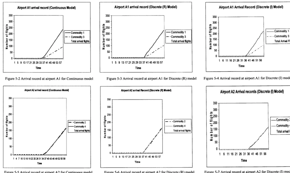
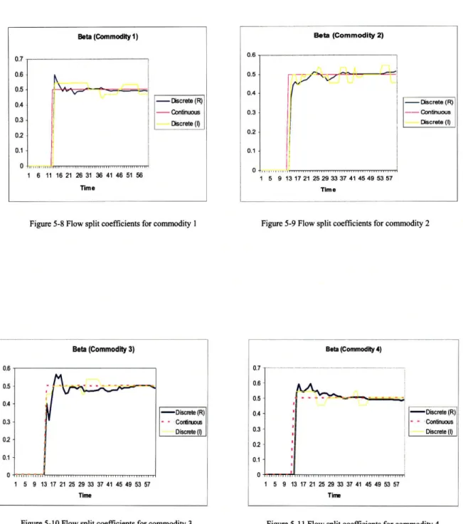
In this case, we consider the network as shown in Figure 5-1 where link 3 and link 4 have the same length of 400 nautical miles. All other parameters are as defined in Section 5.1. The results are summarized in the following tables' and figures:

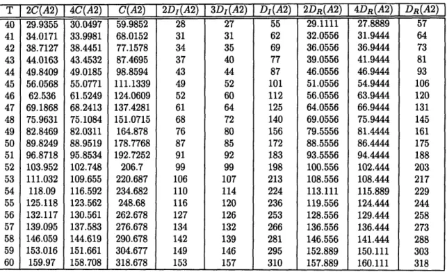
T I 1C(A1) 3C(A1) C(A1) 1DI(A1) 3D1(A1) DI(A1) 1DR(A1) 3DR(A1) DR(A1)

40 37.9243 13.1054 51.0297 30 11 41 33.0556 11.9444 45 41 47.4361 16.5355 63.9716 42 14 56 45.0556 14.9444 60 42 57.1786 20.2005 77.3791 48 17 65 50.0556 18.9444 69 43 66.9983 24.0569 91.0552 57 20 77 59.3889 20.6111 80 44 76.8285 28.0539 104.8824 69 22 91 71.3889 23.6111 95 45 86.6554 32.1377 118.7931 76 28 104 79.3889 30.6111 110 46 96.4906 36.2583 132.7489 82 35 117 85.8889 36.1111 122 47 106.353 40.3752 146.7282 92 39 131 96.3889 40.6111 137 48 116.253 44.4655 160.7185 103 42 145 107.389 44.6111 152.0001 49 126.188 48.5268 174.7148 110 46 156 117.389 49.6111 167.0001 50 136.141 52.5714 188.7124 120 52 172 125.389 56.6111 182.0001 51 146.097 56.6145 202.7115 133 54 187 137.389 59.6111 197.0001 52 156.046 60.6658 216.7118 145 59 204 149.389 62.6111 212.0001 53 165.983 64.7289 230.7119 154 63 217 157.389 69.6111 227.0001 54 175.907 68.8047 244.7117 160 69 229 167.389 74.6111 242.0001 55 185.817 72.8945 258.7115 175 73 248 179.389 77.6111 257.0001 56 195.712 76.9989 272.7109 180 79 259 188.389 83.6111 272.0001 57 205.596 81.1156 286.7116 197 83 280 198.389 86.6111 285.0001 58 215.47 85.2413 300.7113 201 88 289 206.389 91.6111 298.0001 59 225.335 89.376 314.711 212 92 304 217.389 95.6111 313.0001 60 235.185 93.5265 328.7115 220 96 316 227.389 100.611 328

Table 5.1: Comparison of arrival records at destination airport Al (Case I)

1

* T: Time period

* iC(Ai): number of flights of commodity i which arrive at airport Ai in continuous model * iDi(Ai): number of flights of commodity i which arrive at airport Ai in Discrete (I) model * iDR(Ai): number of flights of commodity i which arrive at airport Ai in Discrete (R) model * C(Ai): Total flights arrive at airport Ai in Continuous model

* DI(Ai): Total flights arrive at airport Ai in Discrete (I) model * DR(Ai): Total flights arrive at airport Ai in Discrete (R) model

T I2C(A2) 4C(A2) C(A2) 2DI(A2) 3DI(A2) DI(A2) 2DR(A2) 4DR(A2) DR(A2) 40 25.1397 24.9433 50.083 22 23 45 22 23 45 41 31.3285 31.5547 62.8832 27 29 56 27.0556 29.9444 57 42 37.7431 38.472 76.2151 35 35 70 35.0556 36.9444 72 43 44.3308 45.5351 89.8659 39 41 80 39.0556 43.9444 83 44 51.0866 52.6066 103.6932 47 48 95 47.0556 50.9444 98 45 58.0235 59.5882 117.6117 53 52 105 53.0556 59.9444 113 46 65.1398 66.4343 131.5741 58 57 115 59.0556 68.9444 128 47 72.4039 73.1533 145.5572 66 65 131 67.0556 71.9444 139 48 79.7572 79.7924 159.5496 72 70 142 73.0556 80.9444 154 49 87.132 86.4142 173.5462 83 82 165 83.5556 85.4444 169 50 94.4722 93.0726 187.5448 91 91 182 93.5556 90.4444 184 51 101.748 99.7959 201.5439 97 96 193 98.5556 98.4444 197 52 108.96 106.583 215.543 102 102 204 105.556 106.444 212 53 116.126 113.418 229.544 110 110 220 113.556 112.444 226 54 123.261 120.283 243.544 116 115 231 118.111 119.889 238 55 130.363 127.181 257.544 122 123 245 124.556 128.444 253 56 137.418 134.126 271.544 130 130 260 133.556 133.444 267 57 144.407 141.136 285.543 140 138 278 141.556 140.444 282 58 151.331 148.213 299.544 149 144 293 151.556 145.444 297 59 158.204 155.34 313.544 154 154 308 157.889 154.111 312 60 165.048 162.496 327.544 160 162 322 162.889 164.111 327