The low-resolution CCSM2 revisited: new adjustments and a present-day control run

(1)

HAL Id: hal-00298413

https://hal.archives-ouvertes.fr/hal-00298413

Submitted on 18 Aug 2006

HAL is a multi-disciplinary open access

archive for the deposit and dissemination of sci-entific research documents, whether they are pub-lished or not. The documents may come from teaching and research institutions in France or abroad, or from public or private research centers.

L’archive ouverte pluridisciplinaire HAL, est destinée au dépôt et à la diffusion de documents scientifiques de niveau recherche, publiés ou non, émanant des établissements d’enseignement et de recherche français ou étrangers, des laboratoires publics ou privés.

The low-resolution CCSM2 revisited: new adjustments

and a present-day control run

M. Prange

To cite this version:

M. Prange. The low-resolution CCSM2 revisited: new adjustments and a present-day control run. Ocean Science Discussions, European Geosciences Union, 2006, 3 (4), pp.1293-1348. �hal-00298413�

(2)

OSD

3, 1293–1348, 2006 The low-resolution CCSM2 M. Prange Title Page Abstract Introduction Conclusions References Tables Figures J I J I Back Close

Full Screen / Esc

Printer-friendly Version Interactive Discussion

EGU

Ocean Sci. Discuss., 3, 1293–1348, 2006 www.ocean-sci-discuss.net/3/1293/2006/ © Author(s) 2006. This work is licensed under a Creative Commons License.

Ocean Science Discussions

Papers published in Ocean Science Discussions are under open-access review for the journal Ocean Science

The low-resolution CCSM2 revisited: new

adjustments and a present-day control

run

M. Prange

DFG Research Center Ocean Margins and Department of Geosciences, University of Bremen, Klagenfurter Str., 28334 Bremen, Germany

Received: 26 July 2006 – Accepted: 8 August 2006 – Published: 18 August 2006 Correspondence to: M. Prange (mprange@palmod.uni-bremen.de)

(3)

OSD

Full Screen / Esc

EGU

Abstract

The low-resolution (T31) version of the Community Climate System Model CCSM2.0.1 is revisited and adjusted by deepening the Greenland-Scotland ridge, changing oceanic mixing parameters, and applying a regional freshwater flux adjustment at high northern latitudes. The main purpose of these adjustments is to maintain a robust

5

Atlantic meridional overturning circulation which collapses in the original model re-lease. The paper describes the present-day control run of the adjusted model which is brought into climatic equilibrium by applying a deep-ocean acceleration technique. The accelerated integration is extended by a 100-year synchronous phase. The simu-lated meridional overturning circulation has a maximum of 14×106m3s−1 in the North

10

Atlantic. Most shortcomings found in the control run are identified as “typical problems” in global climate modelling. Given its good simulation skills and its relatively low re-source demands, the adjusted low-resolution version of CCSM2.0.1 appears to be a reasonable alternative to the latest low-resolution Community Climate System Model release (CCSM3.0) if runtime is a critical factor.

15

1 Introduction

Paleoclimatic model experiments usually require long integration times either to reach climatic equilibria which differ from the present-day situation or to simulate long-term (e.g., millennial) climate trends and changes. In order to facilitate long integration times, low-resolution configurations of the fully-coupled NCAR (National Center of

At-20

mospheric Research) Community Climate System Model CCSM have been released both for version 2.0.1 (“CCSM2/T31”) and for version 3.0 (“CCSM3/T31”). In these so-called ‘paleo versions’, the horizontal resolution of the atmospheric component is given by T31 spectral truncation (3.75◦ by 3.75◦ transform grid), whereas the ocean has a nominal resolution of 3.6◦by 1.6◦with 25 levels.

25

(4)

cir-OSD

Full Screen / Esc

EGU

culation in the Atlantic Ocean (Yeager et al., 2006), the Atlantic meridional overturning spins down in CCSM2/T31 such that the net volume export of North Atlantic Deep Water (NADW) to the Southern Ocean drops below 2 Sv (1 Sv=106m3s−1; Fig. 1). As-sociated with the weak overturning circulation is a strong cold bias in the North Atlantic realm (not shown) and the formation of a distinct halocline in the northwest Atlantic

5

where sea surface salinities are several psu below observational values (Fig. 2). This renders CCSM2/T31 unsuitable for paleoclimate studies in which changes of the large-scale deep ocean circulation and the associated meridional heat and salt transports play a crucial role. On the other hand, CCSM3.0 is computationally more expensive than its predecessor CCSM2.0.1, mainly due to physics changes in the atmosphere

10

component (e.g., implementation of explicit transport of two more water species, sed-imentation, and phase changes between condensate species, explicit representation for about 10 species of aerosols, improvements in radiative transfer and cloud overlap). It has been reported that the runtime increase between CCSM3.0 and CCSM2.0.1 can be up to 20% on some distributed-memory machines (M. Renold, University of

15

Bern, personal communication; G. Correa, Lamont-Doherty Earth Observatory, per-sonal communication). Thus, if runtime is a critical factor, CCSM2/T31 could be ad-vantageous over CCSM3/T31, provided that the simulation skill of the meridional over-turning circulation could be improved. In the present paper, it is shown that the perfor-mance of CCSM2/T31 can substantially be improved by applying some modifications

20

to the original model set-up (including the implementation of a regional freshwater flux correction). The low-resolution version of CCSM2.0.1 with these adjustments included is referred to as CCSM2/T31x3a to reflect the atmospheric resolution (“T31”), the av-erage resolution of the ocean grid (“x3”) as well as the implementation of adjustments (“a”). The present paper is devoted to the description of the present-day control run

25

of CCSM2/T31x3a. Since the low-resolution CCSM2.0.1 has already been applied to paleoclimatic problems – both in its original version (Yoshimori et al., 2005, 2006; Raible et al., 2005, 2006) and in its adjusted T31x3a version (Steph et al., 2006) – it is necessary to document the model design in detail.

(5)

OSD

Full Screen / Esc

EGU

The following section describes the tuning of CCSM2/T31x3a. Section 3 describes and discusses the asynchronous integration technique which is used to achieve a sta-tistical equilibrium climate state. The present-day climate from the CCSM2/T31x3a control run is presented in Sect. 4. The focus is placed on oceanic and atmospheric climatological means. The simulation skill for interannual variability in the tropical

Pa-5

cific and North Atlantic regions is briefly discussed. CCSM2/T31x3a’s control run is compared with other models in Sect. 5. Conclusions are drawn in Sect. 6.

2 CCSM2/T31x3a: components and adjustments

The NCAR Community Climate System Model CCSM2.0.1 is composed of four sepa-rate model components: atmosphere, ocean, land and sea ice (Kiehl and Gent, 2004).

10

In a parallel computing environment, these components run simultaneously and com-municate information back and forth via a central coupler. The atmosphere component is the Community Atmosphere Model CAM2, a global general circulation model de-veloped from NCAR’s CCM3. CAM2 employs a spectral dynamical core and hybrid vertical coordinates with 26 levels, combining terrain-following sigma coordinates at

15

the bottom with pressure-level coordinates at the top of the model. The ocean is rep-resented by the z-coordinate, Bryan-Cox type Parallel Ocean Program POP 1.4. The model employs an implicit free surface, an anisotropic viscosity parameterization and Gent-McWilliams isopycnal mixing for tracers using the skew-flux form. A non-local KPP (K-profile parameterization) scheme is applied for vertical mixing. The sea-ice

20

component is the Community Sea-Ice Model CSIM4 with elastic-viscous-plastic dy-namics scheme and an ice thickness distribution module that accounts for 5 ice thick-ness categories. The land component of CCSM2.0.1 is the Community Land Model CLM2. It includes complex biogeophysics and hydrology along with a state-of-the-art river runoff module. Detailed documentations of all model components and parameters

25

– including user’s guides, code reference guides and scientific descriptions – can be found athttp://www.ccsm.ucar.edu/models/ccsm2.0.1.

(6)

OSD

Full Screen / Esc

EGU

In the framework of CCSM, atmosphere and land models share an identical hori-zontal grid. Likewise, ocean and sea ice use one and the same horihori-zontal grid. In CCSM2/T31x3a, the ocean/sea-ice component is formulated on an orthogonal grid which shifts the north pole singularity into Greenland to avoid time-step constraints due to grid convergence. This grid is referred to as “gx3v4” (Fig. 3). It has a

longi-5

tudinal resolution of 3.6◦. The latitudinal resolution of “gx3v4” is variable, with finer resolution (approximately 0.9◦) near the equator.

In CCSM2/T31x3a, several adjustments to the standard CCSM2.0.1 release are ap-plied. The overall goal is to amplify the Atlantic meridional overturning circulation. Due to the computational expense of performing fully-coupled experiments systematic

sen-10

sitivity studies, elucidating the effects of each modification separately, are not feasible for the time being. The tuning of CCSM2.0.1 is based on experience with other models. CCSM2/T31x3a includes the following adjustments:

– The Greenland-Scotland ridge is slightly deepened such that the sill depths are

∼590 m and ∼900 m in the Denmark Strait and in the Iceland-Scotland passage,

15

respectively. Given the vertical resolution of the “gx3v4” ocean grid, these depths are in line with the real bathymetry. A deeper Greenland-Scotland ridge facilitates the exchange of water masses between the North Atlantic and the Nordic Seas where deep winter convection takes place (cf. Koesters et al., 2004).

– Background vertical mixing in the ocean is set to a constant value of 0.3 cm2/s. In

20

the default model set-up vertical background mixing increases from 0.1 cm2/s at the surface to 1.0 cm2/s at 5000 m depth (a value of 0.3 cm2/s is reached at about 2300 m depth). Thus, compared to the default setting, vertical mixing is slightly increased in the upper ocean below the surface boundary layer (alternatively, one could have applied geographically varying upper-ocean parameters with lower

25

vertical diffusivity in the tropics and much higher values in the Southern Ocean where internal wave activity is known to be enhanced, see Gnanadesikan et al., 2006). Vertical mixing provides a mechanism for the conversion of cold deep

(7)

OSD

Full Screen / Esc

EGU

waters into warm water of the upper layers. The crucial role of vertical mixing in driving the thermohaline circulation has been demonstrated in numerous studies (e.g., Bryan, 1987; Wright and Stocker, 1992; Marotzke, 1997; Prange et al., 2003).

– For the Redi and bolus parts of the Gent-McWilliams parameterization diffusivities

5

are set to 1.2×107cm2/s. This represents a 50% increase compared to the de-fault. It is expected that higher horizontal mixing counteracts halocline formation in the northern North Atlantic, thereby favouring convective activity and NADW formation (cf. Schmittner and Weaver, 2001).

– The coefficient used in the quadratic ocean bottom drag formula is increased from

10

10−3to 10−2. The most important effect of this change is a substantial retardation of the flow through the shallow Bering Strait. This throughflow is associated with an import of relatively fresh water from the North Pacific to the Arctic Ocean and the Nordic Seas, where it is likely to affect convective activity. It has been shown in several model studies that a reduction of the Bering Strait throughflow strengthens

15

the meridional overturning circulation in the Atlantic Ocean (e.g., Hasumi, 2002; Wadley and Bigg, 2002; Prange, 2003).

– At each ocean model time step, freshwater fluxes (precipitation plus river runoff)

into the surface grid cells of the Arctic Mediterranean, Labrador Sea and Hudson Bay are reduced by 50%. The corresponding amount of freshwater is

homo-20

geneously distributed over the entire Pacific Ocean (Fig. 4). This leads to an effective sea surface salinity increase in regions that are potentially important for NADW formation. Beyond these regions, the hydrological cycle is simulated with-out unphysical adjustments. This is a main advantage over the more common application of global flux-correction fields. The regional freshwater flux

adjust-25

ment requires modifications in the POP Fortran code and it is presumably the most substantial change to the standard model set-up. Note that neither heat nor momentum flux corrections are implemented in CCSM2/T31x3a.

(8)

OSD

Full Screen / Esc

EGU

In addition to the model tuning which aims at boosting the Atlantic overturning circu-lation, optimized sea-ice/snow albedos are applied based on results from stand-alone sea-ice model experiments: Maximum albedos for thick, dry sea ice are set to 0.82 and 0.38 for the visible and near-infrared spectral band, respectively. The near-infrared albedo for dry snow is set to 0.74. No distinction is made between the hemispheres.

5

3 Accelerated integration

Accelerated integration techniques are often applied to climate models to reduce the computational expense. In order to obtain a present-day climatic equilibrium, a deep-ocean acceleration technique – which is highly efficient in the framework of CCSM2/T31x3a – is employed here. This approach allows for increasing tracer time

10

steps with depth, exploiting the relaxation of the Courant-Friedrichs-Lewy constraint due to diminishing current speeds in the deep ocean (Bryan and Lewis, 1979; Bryan, 1988). Such an asynchronous integration technique has proven useful for searching equilibrium solutions without any interest in the transient behaviour of the model: Once an equilibrium is reached (i.e., vanishing time-derivates in the model equations), the

15

solution is independent of the time-stepping.

However, numerical acceleration techniques can severely distort the model physics. Two major concerns have been raised regarding asynchronous deep-ocean time-stepping. Firstly, this approach does not ensure tracer conservation. Conservation of heat and salt is violated whenever vertical fluxes occur between neighbouring grid

20

boxes that solve the prognostic tracer equations with different time steps (Danaba-soglu et al., 1996). Secondly, time-derivates never vanish in a realistically forced ocean model due to intra- and interannual variability. In order to quantify these er-rors, Danabasoglu (2004) recently applied accelerated integration methods to POP 1.4 subject to realistic forcing. Comparing equilibrium temperatures and salinities obtained

25

by deep-ocean acceleration with those from a 10 000-year synchronous control run, he found that errors are of order 0.1 K and 0.1 psu, respectively, provided that two

(9)

condi-OSD

Full Screen / Esc

EGU

tions are met: (i) vertical variations in time step are restricted to depths where vertical tracer fluxes (i.e. vertical gradients) are small enough that tracers are conserved well enough (in particular below the pycnocline); (ii) the accelerated integration is extended by a synchronous phase of – at least – several decades (Danabasoglu et al., 1996; Wang, 2001; Danabasoglu, 2004). The synchronous extension is important not only

5

to correctly capture oceanic variability, but also to test the stability and reliability of the accelerated equilibrium solution (cf. Bryan, 1984; see also Sect. 4.1). Previous modelling studies have demonstrated the ability of acceleration techniques to reach an equilibrium paleoclimatic solution (see, e.g., Huber and Sloan, 2001; Huber and Nof, 2006).

10

The acceleration-induced small errors found by Danabasoglu (2004) are tolerable for most paleoclimatic applications. In particular, errors in large-scale oceanic mass and heat transports turned out to be negligible (for instance, the error in maximum Atlantic northward heat transport was about 0.01 PW or 1–2%). Using the same oceanic model grid as in the study by Danabasoglu (2004), a similar deep-ocean acceleration scheme

15

is used here. The surface time step in the ocean model is set to 1 h (time-step re-striction due to numerical instability) and does not change down to a depth of 1300 m. Below 2500 m, the tracer time step is increased by a factor 50. Between 1300 m and 2500 m, the tracer time step has a linear variation.

4 Present-day control run

20

4.1 Experimental design and spin-up

For the present-day control run of CCSM2/T31x3a, the atmospheric composition of 1990 AD is adopted. Volume mixing ratios of greenhouse gases are listed in Table 1. The total aerosol visible optical depth is set to 0.14, while a value of 1365 W/m2is used for the solar constant. The model is initialized with observational data sets provided at

25

(10)

OSD

Full Screen / Esc

EGU

Using the deep-ocean acceleration technique described in the previous section, a climatic equilibrium can be achieved within a few centuries of integration. After a short (7 years) synchronous spin-up phase, depth-accelerated integration is applied for 293 years, followed by a centennial synchronous extension. This gives a total integration time of 400 surface years for the coupled climate model corresponding to 14 757

deep-5

ocean years. Only the third stage of the integration procedure (i.e. the centennial synchronous phase) shall serve for an evaluation of the simulated present-day climate. Figure 5 shows the time series of global ocean temperature over the accelerated spin-up phase and the synchronous extension. Initialized with climatological data (Steele et al., 2001) the ocean cools by about 0.6 K until reaching a near-equilibrium

10

state. During the same time, global average salinity increases by about 0.01 psu (not shown). This salinity drift is mainly attributable to the non-conservative character of deep-ocean acceleration.

The Hovm ¨oller diagrams in Fig. 6 display the time evolution of zonally and merid-ionally averaged potential temperature and salinity for the Atlantic, Pacific, and Indian

15

oceans. It is clearly visible that the global oceanic cooling (Fig. 5) can be ascribed to a decrease in deep and bottom water temperatures, while the upper layers gradually warm during the spin-up. The abyssal potential temperature drift during the last cen-tury of accelerated integration (i.e. between surface year 200 and 300) is below 0.1 K, i.e. smaller than 2×10−5K per deep-water year. For the same time interval, abyssal

20

salinity changes are about 0.03 psu or 6×10−6psu per deep-water year. These rates are sufficiently small, confirming that the climatic state is at equilibrium for practical purposes at the end of the accelerated spin-up phase.

Starting from an ocean at rest, most mass (or volume) transports obtain quasi-equilibrium within 50 surface years. Figure 7 shows the temporal evolution of the

25

Atlantic meridional overturning streamfunction at 25◦S. At equilibrium, almost 12 Sv of deep water are exported to the Southern Ocean between 1000 and 3000 m depth; below 3000 m, 2–3 Sv of Antarctic Bottom Water (AABW) enter the Atlantic Ocean. The major goal of model tuning is achieved: CCSM2/T31x3a produces a robust overturning

(11)

OSD

Full Screen / Esc

EGU

circulation in the Atlantic Ocean which induces a substantial northward heat transport (cf. Sect. 4.2.1). In this stable climatic mode, the northern high-latitude freshwater flux correction totals 0.107 Sv (averaged over the last 100 years of the integration period).

The largest transport of water in the world ocean occurs within the Antarctic Cir-cumpolar Current (ACC). The volume transport through Drake Passage rapidly

equi-5

librates during model spin-up approaching 90 Sv (Fig. 8). It is important to note that the time series of oceanic volume transports provide a hint on the stability and reliabil-ity of the accelerated equilibrium solution (cf. Peltier and Solheim, 2004). Large-scale volume transports (like the meridional overturning circulation or the ACC) quickly re-spond to changes in the forcing, generally adjusting within a few decades (e.g., Gerdes

10

and Koeberle, 1995; Danabasoglu et al., 1996). If the accelerated integration led to a “false equilibrium”, a rapid reorganisation of the oceanic volume transports would be expected after switching from accelerated to synchronous integration at year 300 (which is obviously not the case).

4.2 Equilibrium climatology

15

4.2.1 Ocean

For the following evaluation of the CCSM2/T31x3a present-day climatic equilibrium, the last 90 years of the synchronous integration phase are considered; that is, averages from surface years 311–400 are calculated and compared to observational climatolo-gies or observation-based estimates.

20

Some important integrated measures for the world ocean circulation are listed in Ta-ble 2 and compared with estimates from inverse (Ganachaud and Wunsch, 2000) and data-constrained (Stammer et al., 2003) modelling. While the Indonesian Througflow (ITF) and the transport of Pacific Water into the Arctic Ocean through Bering Strait (cf. Sect. 2) are well captured by the model, the simulated mass transport of the ACC

25

is 25–30% smaller than observation-based estimates. Although the total transport of the ACC is governed by both wind stress and buoyancy fluxes (Gent et al., 2001; Olbers

(12)

OSD

Full Screen / Esc

EGU

et al., 2004), a too weak zonal wind forcing at ACC latitudes is most likely responsi-ble for the shortcoming in CCSM2/T31x3a (cf. Sect. 4.2.3). The maximum meridional overturning strength in the North Atlantic appears to be in line with observation-based estimates. Note, however, that only 60% of deep-water formed in the North Atlantic is exported to the Southern Ocean (Fig. 9). Accordingly, the Atlantic Ocean northward

5

heat transport simulated by CCSM2/T31x3a is at the lower end of the range suggested by observations. In addition, the flow of NADW is relatively shallow and the total for-mation of AABW is weak (Fig. 9). For comparison: Ganachaud and Wunsch (2000) estimate a northward AABW flow of 5–7 Sv into the Atlantic, 4–12 Sv into the Indian, and 5–9 Sv into the Pacific Ocean.

10

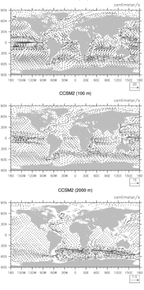
The horizontal distribution of ocean mean currents is displayed in Fig. 10. In the surface layer, the equatorial Pacific is dominated by Ekman-driven divergent flow. At 100 m depth, swift equatorial undercurrents, flowing eastward, are visible in all three oceans. In the Pacific Ocean, the Equatorial Undercurrent is supplied by meridional geostrophic inflow that compensates the Ekman transports, including inflows at the

15

western boundary. In the Indian Ocean, the eastward current is mainly fed by the South Equatorial Current which, in turn, is supplied by the subtropical gyre circulation and the ITF. In accordance with observations, the ITF receives water basically from the Pacific North Equatorial Current (cf. Gordon, 2001). The Atlantic Equatorial Undercurrent is mainly fed from the South Atlantic (South Equatorial Current).

20

The Benguela Current, appearing below the Ekman layer, separates from the African coast far too south. Similar problems arise with other eastern boundary currents (e.g., the Humboldt Current). Given the rather coarse resolution of the model grid, subtropical western boundary currents – including Kuroshio, Gulf Stream, East Australian Current, Mozambique Current, and Brazil Current – are simulated satisfactorily. As in reality, the

25

Brazil Current is conspicuously weak as compared with the other western boundary currents (cf. Peterson and Stramma, 1991).

At high southern latitudes, the flow field is dominated by the ACC. South of the ACC, the westward flowing Antarctic Coastal Current is simulated. Around the southern tip

(13)

OSD

Full Screen / Esc

EGU

of Africa, the model version of the Agulhas Current/leakage transports water from the Indian Ocean to the South Atlantic. This transport may be an integral part of the global conveyor belt circulation (Gordon, 1986). In the North Atlantic, a strong North Atlantic Current marks the boundary between the subtropical gyre and the cyclonic subpolar gyre. Providing the convective regions south of Greenland and in the Nordic Seas

5

with warm and salty water, the simulation of the North Atlantic Current is of utmost importance for the thermohaline circulation.

The flow field at 2000 m depth is characterized by a vigorous circulation around Antarctica. In the Atlantic Ocean, the southward movement of NADW constitutes the lower limb of the thermohaline overturning circulation. The NADW flow path forms an

10

anticyclonic loop in the North Atlantic, which has no counterpart in observations. South of 30◦N, the southward flow of NADW is confined to the Deep Western Boundary Cur-rent.

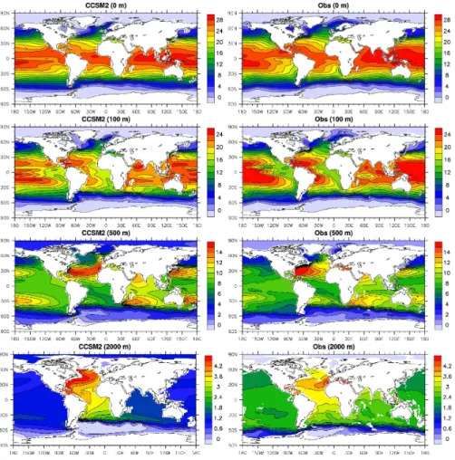
Potential temperatures simulated by CCSM2/T31x3a are shown in Fig. 11 along with observational data. Modelled sea surface temperatures (SST) in the tropical Indian

15

and Pacific oceans are lower than observed. This cold bias is up to 2 K in the equa-torial central Pacific. The cold surface temperatures are associated with a larger than observed low-level cloud cover over the equatorial Pacific (not shown). In the tropi-cal Atlantic, the western warm pool is too cold and the zonal SST gradient has the wrong sign. The tropical cold temperature bias is also visible at 100 m depth. The most

20

pronounced deficiencies at subtropical latitudes are found in the eastern boundary currents and major upwelling regions (along the west coasts of North America, South America, northwest Africa, and southwest Africa), where surface and subsurface tem-peratures are too warm. In northern high latitudes, the North Atlantic Current provides for moderate water temperatures south of Iceland and in the Norwegian Sea.

Com-25

pared to the standard CCSM2.0.1 low-resolution control run (not shown), the model adjustments result in upper-ocean temperatures in the northern North Atlantic that are much more in line with observations. At 500 m depth, the modelled Pacific, Indian and North Atlantic subtropical gyres exhibit higher temperatures compared to

(14)

obser-OSD

Full Screen / Esc

EGU

vations, whereas the subtropical South Atlantic is slightly too cold in CCSM2/T31x3a. At 2000 m in the North Atlantic, simulated NADW has a potential temperature of about 4.5◦C. Deep temperatures in the Pacific and Indian oceans are ∼1 K colder than in ob-servations, pointing to a cold bias in AABW. A similar deep-ocean cold bias has been found in the higher resolution (T42) version of the model (Kiehl and Gent, 2004).

5

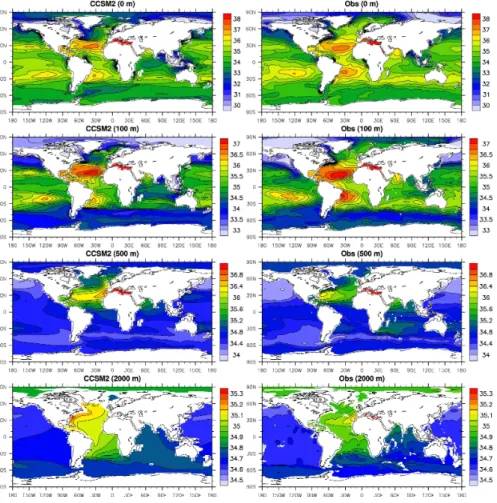
Figure 12 shows global salinity fields. The success of the CCSM2/T31x3a model adjustments is most evident when comparing the field of annual-mean sea surface salinity with that from the standard CCSM2.0.1 control run (Fig. 2). The entire North Atlantic, including subtropical and subpolar regions as well as the Nordic Seas and the Arctic Ocean, exhibits surface salinities which are now much closer to observations.

10

However, low-salinity water still caps off the Labrador Sea, forcing convection to occur further to the east. The reason for this shortcoming is unclear. Deficiencies in the wind stress curl, however, are likely to play a crucial role in the formation of the Labrador low-salinity cap (Gnanadesikan et al., 2006). In the Nordic Seas and northern North Atlantic, winter convection and, hence, deep-water formation takes place where

upper-15

ocean salinities are around or above 35 psu.

In the South Atlantic, the model exhibits an upper-ocean fresh bias. The subtropical front is marked by the 34.9 psu isohaline at 100 m depth. In observations, the front resides well to the south of the Cape of Good Hope and the Australian continent. In CCSM2/T31x3a, the subtropical front is shifted far to the north (cf. Fig. 12). Part of

20

this fresh bias can be attributed to excessive rainfall between 35◦S and 60◦S (see Fig. 19). In the southeastern Atlantic, a possible source of error is the lack of Agulhas eddies that transport salty water into the Atlantic. A much finer grid resolution would be required to simulate the formation of these eddies.

Relatively high salinities are found in the North Pacific, whereas the upper Indian

25

Ocean is overly fresh. In particular, the salinity of Australasian Mediterranean Water (AAMW) at the surface (at 100 m depth) is about 1 psu (0.5 psu) below observational values. At 500 m depth, the signature of AAMW is well captured by the model, still the region around Madagascar is too fresh. The salinity field at 2000 m reveals somewhat

(15)

OSD

Full Screen / Esc

EGU

saltier NADW in the model compared to observations. Traces of Eurafrican Mediter-ranean Water are absent at 2000 m depth in both the temperature (Fig. 11) and salinity (Fig. 12) fields of the model.

4.2.2 Sea ice

Maximum and minimum sea-ice conditions in the northern and southern hemispheres

5

simulated by CCSM2/T31x3a are displayed in Fig. 13. The use of optimized sea-ice/snow albedos in CCSM2/T31x3a leads to an ice thickness of 2.5–3.5 m over the central Arctic Ocean. North of Greenland the sea-ice thickness increases up to 6 m. These results are in good agreement with upward-looking sonar observations (e.g., Bourke and Garrett, 1987) and satellite altimeter measurements (Laxon et al., 2003).

10

In the Arctic Ocean proper, the largest discrepancy between model and data is found along the East Siberian coast, where the model predicts ice thicknesses similar to those north of Greenland, while observations suggest thin ice (<1 m) or even ice-free conditions during specific summer months. The overly thick ice cover along the East Siberian coast can mainly be attributed to a deficient wind-stress forcing. A negative

15

sea-level pressure (SLP) bias over Alaska and northwestern Canada (cf. Fig. 16) forces sea ice to drift from the North American coast towards East Siberia, thus maintaining an unusually thick ice-cover in that region. In the North Atlantic and the Nordic Seas, the model produces too much ice area. Most severly affected in winter are the Labrador Sea, the regions east and northeast of Iceland, the sector south of Svalbard as well

20

as the western Barents Sea. The model reproduces year-round ice-free conditions over almost the entire Norwegian Sea. During the summer months, CCSM2/T31x3a simulates too much sea ice south of Greenland, around Svalbard, and in Baffin Bay. In the Southern Ocean, the overall pattern of sea-ice cover is simulated satisfacto-rily. Although the model produces excessively thick ice along the eastern coast of the

25

Antarctic Peninsula, the typical “boomerang shape” thickness distribution in the Wed-dell Sea is qualitatively captured (cf. Strass and Fahrbach, 1998). As in the northern hemisphere, CCSM2/T31x3a exhibits a bias towards extensive sea-ice cover in the

(16)

OSD

Full Screen / Esc

EGU

Atlantic sector. This is particularly true for the Scotia Sea. 4.2.3 Atmosphere

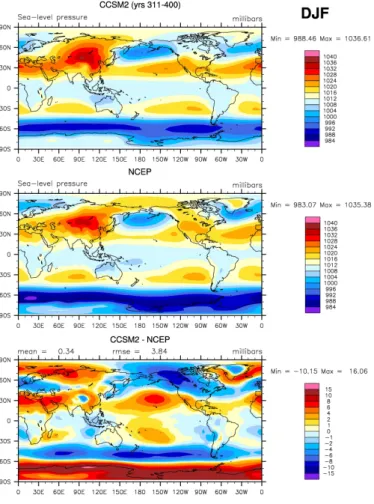
The overall performance of CCSM2/T31x3a with respect to the climatology of atmo-spheric basic surface variables (SLP, reference height air temperature, precipitation) is described in the following. Figure 14 displays the geographical mean pattern of

5

December–February (DJF) SLP simulated by the model against NCEP reanalysis data. The core positions of subpolar lows and subtropical highs are generally well captured in CCSM2/T31x3a, although the centers of the Icelandic Low and Azores High are slightly displaced eastward relative to observations. The strengths of the subtropical highs are overestimated in the northern hemisphere, and underestimated in the southern

hemi-10

sphere. Anomalously high pressure is found in Arctic and sub-Arctic regions, where the model produces too much sea ice and too cold surface air temperatures (Labrador Sea, Greenland Sea, Barents Sea). Over Canada, the simulated winter pressure is lower than observed by up to 9 hPa. In high southern latitudes, the model exhibits a low pressure-bias over the subpolar seas, and a high-pressure bias over the Antarctic

15

continent.

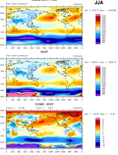
During June–August (JJA) the simulated strengths of subtropical highs are close to reanalysis data in the southern hemisphere (Fig. 15). In the northern hemi-sphere, CCSM2/T31x3a exhibits a pronounced high-pressure bias over the mid-latitude oceans. In the Arctic realm, the simulated SLP is more than 6 hPa larger than

20

in NCEP data with a maximum deviation over Greenland. Antarctic and sub-Antarctic regions in the model climate are characterized by a strong low-pressure bias relative to reanalysis data. A similar seasonality of the Antarctic SLP bias (high pressure during DJF, low pressure during JJA) has been found in other climate models (e.g., Min et al., 2004). It should be noted, however, that errors in the reanalysis data cannot be

25

excluded for these extreme regions.

The deviation in simulated annual-mean SLP (Fig. 16) is associated with anoma-lously weak westerlies at the latitude of Drake Passage relative to NCEP data. The poor

(17)

OSD

Full Screen / Esc

EGU

simulation of Southern Ocean wind forcing may partly be responsible for the low volume transport in the ACC. Moreover, it may partly account for the model’s bias towards a weak Atlantic meridional overturning circulation (cf. McDermott, 1996; Gnanadesikan, 1999).

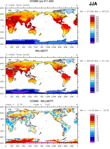
The geographical pattern of DJF 2-m air temperature over land is shown in

5

Fig. 17. On global average, the simulated DJF temperature is 0.28 K greater than the observation-based (1950–1999) estimate. The winter surface climate of CCSM2/T31x3a is too warm over Greenland, northeastern Asia, and northern North America. The North American warm bias is associated with a low SLP anomaly (Fig. 14). During the summer season, simulated air temperatures are in better

agree-10

ment with observations, and the global average is only 0.16 K warmer (Fig. 18). An overall cold bias for African and South American climates, however, is visible in both seasons. The same holds true for a pronounced warm bias over Antarctica. On annual average, the global 2-m air temperature over land is 0.1 K larger in CCSM2/T31x3a than in observations, while the global root-mean-square error (rmse) amounts to

15

3.35 K.

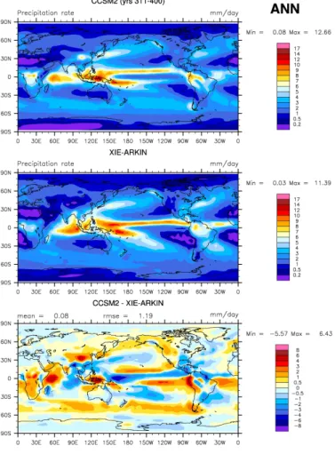
A comparison of the simulated geographical distribution of annual-mean precipitation rate with CMAP observations is displayed in Fig. 19. The warm-biased region of north-western North America receives excessive precipitation in CCSM2/T31x3a. The same holds for northeastern Siberia, albeit with a smaller magnitude of the error. Pronounced

20

wet biases are also visible over the central and southern parts of Africa, northern China, southern India, and eastern Indonesia, while Mainland Southeast Asia is too dry in the model. On the eastern side of the tropical Pacific, the model underestimates precipita-tion over central America and northern South America, while the coastal areas of Peru and Ecuador are too wet. Over the tropical ocean, the difference plot between model

25

and data reveals several shortcomings in the simulation: an east-west dipole over the Indian Ocean, a north-south dipole over the equatorial Atlantic owing to a rather dif-fuse Atlantic Intertropical Convergence Zone (ITCZ) in the model annual average, and a “double ITCZ” in the eastern Pacific. The “double ITCZ” emerges from a spurious

(18)

OSD

Full Screen / Esc

EGU

zonal band of excess rainfall just south of the equator, whereas the observations re-veal a maximum extending from the west Pacific warm pool south-eastwards towards French Polynesia (the South Pacific Convergence Zone).

Figure 20 shows the mean annual cycle of zonally averaged precipitation as de-rived from the model and CMAP data. While the major meridional shift in observed

5

tropical precipitation from the southern to the northern hemisphere takes place from March to April, it occurs between May and July in the model. During that time, zonal-average CCSM2/T31x3a precipitation shows a false double structure of the ITCZ. In observations, the zonally averaged precipitation rate has a northern hemisphere max-imum from June to August. In the model, the northern hemisphere maxmax-imum occurs

10

in September and is somewhat smaller than observed. In northern hemisphere mid-latitudes, the seasonal variation of precipitation is overestimated by the model. In the southern hemisphere, CCSM2/T31x3a has a year-round dry bias around 30◦S, and a wet bias around 50◦S (see also Fig. 19).

4.2.4 Total heat transport

15

Annual averaged meridional heat transports by the ocean, the atmosphere, and the coupled system are displayed in Fig. 21 and compared with NCEP-derived values. In CCSM2/T31x3a, the maximum meridional ocean heat transport is 1.3 PW in the north-ern hemisphere, and 1.2 PW in the southnorth-ern hemisphere. These transports are about 0.5 PW smaller than NCEP-derived values. Maximum meridional heat transports in the

20

atmosphere model are 4.9 PW and 5.4 PW in the northern and southern hemisphere, respectively. While the northern-hemisphere value is in good agreement with reanal-ysis, the southern hemisphere atmospheric transport is about 0.5 PW larger than the NCEP-derived value.

(19)

OSD

Full Screen / Esc

EGU

4.3 Climate variability 4.3.1 Tropical Pacific

Tropical climate variability on the short-range timescale from a few months to several years is dominated by the El Ni ˜no/Southern Oscillation (ENSO). Figure 22 shows the wavelet power spectrum of the Ni ˜no-3.4 index (SST 5◦S–5◦N, 170◦W–120◦W)

calcu-5

lated from the synchronous integration phase of the CCSM2/T31x3a control run. The global wavelet power spectrum exhibits a maximum around 2 years, while the ENSO period deduced from observational data has a broader spectral peak near 3–7 years. In harmony with observations, tropical interannual variability strongly varies from decade to decade (cf. Latif, 1998).

10

For a closer inspection of tropical Pacific variability, Fig. 23 displays Hovm ¨oller plots of equatorial SST and 850-hPa zonal-wind anomalies. A 20-year interval has been chosen which includes two very strong El Ni ˜no events (years 366/367 and 368/369) and a phase of reduced ENSO frequency (years 370–378). Comparing the SST anomalies with the 850-hPa zonal-wind anomalies reveals a strong atmosphere-ocean coupling in

15

the model tropics. Wind anomalies are particularly pronounced during the two strong El Ni ˜no events as well as during the two strong cold La Ni ˜na events in years 365/366 and 370. Compared to observations, the amplitude of SST variations is too small in the model tropical Pacific. Moreover, CCSM2/T31x3a simulates the strongest SST fluctuations in the central part of the basin, while SST variability in the eastern Pacific is

20

substantially underestimated. Likewise, maximum zonal-wind anomalies are situated too far in the west compared to observations.

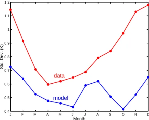
It has been shown by Latif et al. (2001) and AchutaRao and Sperber (2002) that many climate models are not capable of simulating ENSO’s phase locking to the an-nual cycle. To test the skill of CCSM2/T31x3a in simulating the seasonal cycle

phase-25

locking, the interannual standard deviations of the Ni ˜no-3.4 SST anomalies are calcu-lated as a function of calendar month (Fig. 24). Although CCSM2/T31x3a simulates a secondary maximum in August, the strongest variability occurs during boreal

(20)

win-OSD

Full Screen / Esc

EGU

ter. It is therefore concluded that, compared to other models, CCSM2/T31x3a shows reasonably good skill in simulating the seasonal cycle phase-locking.

4.3.2 North Atlantic

Climate variability in the North Atlantic and European realm is strongly linked to the North Atlantic Oscillation (NAO), the most prominent mode of variability in northern

5

hemisphere winter climate. Here, the leading large-scale pattern associated with the NAO is extracted by principal component analysis on the winter 500-hPa geopotential height field, considering a limited spatial domain (90◦W–30◦E, 20◦N–80◦N). Figure 25 shows the leading empirical orthogonal function (EOF) obtained from the synchronous integration phase of the CCSM2/T31x3a control run. The first EOF accounts for 58.5%

10

of the total 500-hPa geopotential height variance over the spatial domain. This number is somewhat higher than the value calculated from NCEP reanalysis data (49.4%). The 500-hPa height pattern consists of two centers-of-action. The northern center-of-action is captured well by the model. The southern center is less well simulated, being displaced too far west and too far south over the Atlantic Ocean.

15

5 Discussion

CCSM2/T31x3a produces an overall reasonable present-day global climate. Neverthe-less, the evaluation of the control run has revealed several shortcomings. Most of these shortcomings are well known as “typical problems” (i.e. common biases) in global, non-flux-corrected climate models. A strong surface cold bias in the equatorial Pacific, a

20

wrong sign of the tropical Atlantic zonal SST gradient, and positive SST biases at the eastern boundaries of the subtropical Pacific and Atlantic ocean basins (coastal up-welling regions of North/South America, northwestern/southwestern Africa) were to be expected from the history of ocean climate modelling (Mechoso et al., 1995; Latif et al., 2001; AchutaRao and Sperber, 2002; Davey et al., 2002; Wittenberg et al., 2006).

(21)

OSD

Full Screen / Esc

EGU

Sensitivity experiments suggest that errors in both surface solar radiation (through an under-prediction of stratus clouds in the atmosphere model) and wind stress ocean forcing (driving the coastal upwelling of cold thermocline water through surface Ekman divergence) each contribute about one-half to the common eastern boundary SST bias in climate models (Kiehl and Gent, 2004; Large and Danabasoglu, 2006). The

repre-5

sentation of narrow coastal upwelling is also strongly dependent on the spatial resolu-tion of the oceanic model grid. However, increasing the resoluresolu-tion of the ocean model does not necessarily reduce the SST biases in coastal upwelling regions (Yeager et al., 2006). It is important to note that eastern boundary surface biases are probably not confined locally. They can rather be advected over large distances and, hence, may

10

exert large-scale, remote influences over the coupled solution, even contributing to the double ITCZ problem (Li et al., 2004; Kiehl and Gent, 2004; Large and Danabasoglu, 2006).

The rainfall double ITCZ is a common problem in coupled non-flux-corrected cli-mate models (Mechoso et al., 1995; Lambert and Boer, 2001; Harvey, 2003; Covey

15

et al., 2003; Li et al., 2004; Dai, 2006). A better simulation of the surface hydrogra-phy in the east Pacific coastal upwelling regions might improve the spatial structure of tropical rainfall. Recently, Zhang and Wang (2006) demonstrated that the use of a modified Zhang-McFarlane convection scheme significantly mitigates the double ITCZ problem in CCSM3.0, also resulting in an improvement of the Pacific SST simulation.

20

The annual-mean dry/wet bias over eastern/western equatorial Indian Ocean and a northern hemisphere mid-latitude wet bias in winter are other typical precipitation er-rors present in many coupled models (Lambert and Boer, 2001; Covey et al., 2003). Likewise, annual warm biases over Antarctica and Greenland as well as winter (DJF) warm biases over northeastern Asia and northern North America are often found in

25

climate models (Lambert and Boer, 2001; Covey et al., 2003).

The movement and distribution of sea ice is strongly determined by the high-latitude wind field. Excessive ice build-up along the Siberian coast is mainly attributable to an erroneous Arctic wind field and has been identified to be another common problem in

(22)

OSD

Full Screen / Esc

EGU

many climate models (Bitz et al., 2002; DeWeaver and Bitz, 2006).

The skill of models to simulate interannual variability in the tropical Pacific has been analysed in various studies. It has been found that most global climate models tend to produce ENSO-like variability that occurs at a higher-than-observed frequency (period-icity of 2–3 years instead of 3–7 years), and that most models are placing the maximum

5

SST variability in the equatorial Pacific too far to the west (Latif et al., 2001; Davey et al., 2002; AchutaRao and Sperber, 2002). Although the latest climate models tend to be more realistic in representing the frequency with which ENSO occurs, and they are bet-ter at locating enhanced SST variability over the easbet-tern Pacific (van Oldenborgh et al., 2005; AchutaRao and Sperber, 2006), CCSM2/T31x3a’s skill to simulate interannual

10

variability in the tropical Pacific is well within the range of other models. Teleconnection patterns associated with ENSO in CCSM2/T31x3a will be analysed elsewhere.

None of the above mentioned problems disappears in the higher-resolution (T42) version of CCSM2.0.1 or in the latest model release, CCSM3.0. Basically, control runs of CCSM2/T42, CCSM3/T31, CCSM3/T42 (and even CCSM3/T85) still suffer from the

15

same shortcomings with respect to precipitation, sea/land surface temperatures, sea-ice distribution (in both hemispheres) and tropical climate variability (see Kiehl and Gent, 2004; Yeager et al., 2006; Holland et al., 2006; Deser et al., 2006; DeWeaver and Bitz, 2006). Even though the winter surface warm bias over northeastern Asia and northern North America is reduced in CCSM3/T31 compared to CCSM2/T31x3a, the

20

errors are similar in the higher resolution versions CCSM3/T42 and CCSM3/T85 (see

http://www.ccsm.ucar.edu/experiments). Table 3 summarizes errors of some globally averaged climatological quantities for different versions of the Community Climate Sys-tem Model. Different climate variables are simulated with different levels of success by the different models and no one model is best for all variables.

25

While CCSM2/T42, CCSM3/T31, and CCSM3/T42 do not include any flux adjust-ments, the main disadvantage of CCSM2/T31x3a is the need for a freshwater flux ad-justment at high northern latitudes in order to produce a robust Atlantic meridional over-turning circulation. However, since this flux adjustment is limited to the Arctic

(23)

Mediter-OSD

Full Screen / Esc

EGU

ranean, Labrador Sea and Hudson Bay, the model behaves like a non-flux-corrected model with respect to tropical and subtropical climate dynamics and variability. This is particularly crucial when ENSO dynamics are considered (cf. AchutaRao and Sperber, 2002; Davey et al., 2002).

It is important to note that the implementation of a freshwater flux adjustment is

5

not a step backwards compared to the older version of the climate system model, CSM1, which is often considered as a “non-flux-corrected” model (e.g., Latif et al., 2001; AchutaRao and Sperber, 2002; Covey et al., 2003; Stephenson and Pavan, 2003). However, CSM1 has no river runoff scheme. Instead, the precipitation over the ocean is multiplied by a factor to allow for a global surface freshwater balance. In

10

so doing, CSM1 gets rid of the huge input of river water into the Arctic Mediterranean which – as the largest source of freshwater to the northern high-latitude seas – is about 0.1 Sv (Prange and Gerdes, 2006, and references therein). Therefore, at high northern latitudes, CSM1’s simplification of the hydrological cycle has a very similar effect on the oceanic freshwater forcing than the flux adjustment applied to CCSM2/T31x3a.

15

6 Conclusions

The low-resolution version (“paleo version”) of CCSM2.0.1 has been revisited. The original release has been adjusted by deepening the Greenland-Scotland ridge, chang-ing oceanic mixchang-ing parameters, and applychang-ing a regional freshwater flux adjustment at high northern latitudes. The overall goal of these model adjustments, i.e. the

improve-20

ment of the Atlantic meridional overturning circulation, has been achieved.

In the present paper, important aspects of the present-day control run of the ad-justed version, CCSM2/T31x3a, have been critically analysed, and major shortcomings have been exposed. This provides a basis from which to judge numerical experiments performed with CCSM2/T31x3a. Most biases found in the CCSM2/T31x3a control

25

run have been identified as “typical problems” in global climate modelling. Given its good simulation skills and its relatively low resource demands, CCSM2/T31x3a shows

(24)

OSD

Full Screen / Esc

EGU

promise for studies of paleoclimate and other applications requiring long integrations and equilibrated solutions. For researchers who have no or only strongly limited access to shared-memory supercomputers, the higher runtime of CCSM3.0 on distributed-memory machines could be critical such that CCSM2/T31x3a appears to be a reason-able alternative to CCSM3/T31. In this context, it is worth noting that a Linux version of

5

CCSM2.0.1 is provided by the Climate and Environmental Physics group at the Univer-sity of Bern (Renold et al., 2004). Nevertheless, for applications in which variations of the Arctic Ocean freshwater budget play a crucial role, special care should be taken due to the implementation of the arctic/subarctic flux adjustment. The individual researcher has to decide whether the adjustments applied to CCSM2/T31x3a are acceptable for

10

her/his specific application. This evaluation will necessarily depend on the nature of the phenomenon under investigation.

Acknowledgements. The author is indebted to M. Renold and C. Raible from the Climate

& Environmental Physics Group at the University of Bern for providing their POP analysis software. Thanks is due to M. J. Stevens from the Climate & Global Dynamics Division at

15

NCAR for making the CCSM Diagnostics Package available. The software package can be downloaded fromhttp://www.cgd.ucar.edu/cms/stevens/master.html. The model run was per-formed on the IBM pSeries 690 Supercomputer of the “Norddeutscher Verbund f ¨ur Hoch- und H ¨ochstleistungsrechnen” (HLRN). M. Schulz is greatly acknowledged for his help and support. This work was funded by the Deutsche Forschungsgemeinschaft through the DFG Research

20

Center “Ocean Margins” at the University of Bremen.

References

AchutaRao, K. and Sperber, K. R.: Simulation of the El Ni ˜no Southern Oscillation: Results from the Coupled Model Intercomparison Project, Climate Dyn., 19, 191–209, 2002.

AchutaRao, K. and Sperber, K. R.: ENSO simulation in coupled ocean-atmosphere models:

25

are the current models better?, Climate Dyn., 27, 1–15, 2006.

Bitz, C. M., Fyfe, J. C., and Flato, G. M.: Sea ice response to wind forcing from AMIP models, J. Climate, 15, 522–536, 2002.

(25)

OSD

Full Screen / Esc

EGU

Bourke, R. H. and Garrett, R. P.: Sea ice thickness distribution in the Arctic Ocean, Cold Reg. Sci. Technol., 13, 259–280, 1987.

Bryan, F.: Parameter sensitivity of primitive equation ocean general circulation models, J. Phys. Oceanogr., 17, 970–986, 1987.

Bryan, K.: Accelerating the convergence to equilibrium in ocean-climate models, J. Phys.

5

Oceanogr., 14, 666–673, 1984.

Bryan, K.: Efficient methods for finding the equilibrium climate of coupled ocean-atmosphere models, in: Physically-based modelling and simulation of climate and climate change – Part I, edited by: Schlesinger, M. E., Kluwer Academic Publishers, 567–582, 1988.

Bryan, K. and Lewis, L. J.: A water mass model of the world ocean, J. Geophys. Res., 84,

10

2503–2517, 1979.

Covey, C., AchutaRao, K. M., Cubasch, U., et al.: An overview of results from the Coupled Model Intercomparison Project, Global Planet. Change, 37, 103–133, 2003.

Dai, A.: Precipitation characteristics in eighteen coupled climate models, J. Climate, in press, 2006.

15

Danabasoglu, G.: A comparison of global ocean general circulation model solutions obtained with synchronous and accelerated integration methods, Ocean Model., 7, 323–341, 2004. Danabasoglu, G., McWilliams, J. C., and Large, W.G.: Approach to equilibrium in accelerated

global oceanic models, J. Climate, 9, 1092–1110, 1996.

Davey, M. K., Huddleston, M., Sperber, K. R., et al.: STOIC: a study of coupled model

climatol-20

ogy and variability in tropical ocean regions, Climate Dyn., 18, 403–420, 2002.

Deser, C., Capotondi, A., Saravanan, R., and Phillips, A. S.: Tropical Pacific and Atlantic climate variability in CCSM3, J. Climate, 19, 2451–2481, 2006.

DeWeaver, E. and Bitz, C. M.: Atmospheric circulation and its effect on Arctic sea ice in CCSM3 simulations at medium and high resolution, J. Climate, 19, 2415–2436, 2006.

25

Ganachaud, A. and Wunsch, C.: Improved estimates of global ocean circulation, heat transport and mixing from hydrographic data, Nature, 408, 453–457, 2000.

Gent, P. R., Large, W. G., and Bryan, F. O.: What sets the mean transport through Drake Passage?, J. Geophys. Res., 106, 2693–2712, 2001.

Gerdes, R. and Koeberle, C.: On the influence of DSOW in a numerical model of the

North-30

Atlantic general circulation, J. Phys. Oceanogr., 25, 2624–2642, 1995.

Gnanadesikan, A.: A simple predictive model for the structure of the oceanic pycnocline, Sci-ence, 283, 2077–2079, 1999.

(26)

OSD

Full Screen / Esc

EGU

Gnanadesikan, A., Dixon, K. W., Griffies, S. M., et al.: GFDL’s CM2 global coupled climate models. Part II: The baseline ocean simulation, J. Climate, 19, 675–697, 2006.

Gordon, A. L.: Inter-ocean exchange of thermocline water, J. Geophys. Res., 91, 5037–5046, 1986.

Gordon, A. L.: Interocean exchange, in: Ocean circulation and climate, edited by: Siedler, G.,

5

Church, J., and Gould, J., Academic Press, San Diego, 303–314, 2001.

Harvey, L. D. D.: Characterizing and comparing the control-run variability of eight coupled AOGCMs and of observations. Part 2: precipitation, Climate Dyn., 21, 647–658, 2003. Hasumi, H.: Sensitivity of the global thermohaline circulation to interbasin freshwater transport

by the atmosphere and the Bering Strait throughflow, J. Climate, 15, 2516–2526, 2002.

10

Holland, M. M., Bitz, C. M., Hunke, E. C., Lipscomb, W. H., and Schramm, J. L.: Influence of the sea ice thickness distribution on polar climate in CCSM3, J. Climate, 19, 2398–2414, 2006. Huber, M. and Nof, D.: The ocean circulation in the Southern Hemisphere and its climatic

impacts in the Eocene, Palaeogeogr., Palaeoclimat., Palaeoecol., 231, 9–28, 2006.

Huber, M. and Sloan, L. C.: Heat transport, deep waters, and thermal gradients: Coupled

15

simulation of an Eocene greenhouse climate, Geophys. Res. Lett., 28, 3481–3484, 2001. Kiehl, J. T. and Gent, P. R.: The Community Climate System Model, version 2, J. Climate, 17,

3666–3682, 2004.

Koesters, F., Kaese, R., Fleming, K., and Wolf, D.: Denmark Strait overflow for Last Glacial Maximum to Holocene conditions, Paleoceanogr., 19, PA2019, doi:10.1029/2003PA000972,

20

2004.

Lambert, S. J. and Boer, G. J.: CMIP1 evaluation and intercomparison of coupled climate models, Climate Dyn., 17, 83–106, 2001.

Large, W. G. and Danabasoglu, G.: Attribution and impacts of upper-ocean biases in CCSM3, J. Climate, 19, 2325–2346, 2006.

25

Latif, M.: Dynamics of interdecadal variability in coupled ocean-atmosphere models, J. Climate, 11, 602–624, 1998.

Latif, M., Sperber, K., Arblaster, J., et al.: ENSIP: the El Ni ˜no simulation intercomparison project, Climate Dyn., 18, 255–276, 2001.

Laxon, S., Peacock, N., and Smith, D.: High interannual variability of sea ice thickness in the

30

Arctic region, Nature, 425, 947–950, 2003.

Li, J. L., Zhang, X. H., Yu, Y. Q., and Dai, F. S.: Primary reasoning behind the double ITCZ phenomenon in a coupled ocean-atmosphere general circulation model, Adv. Atmos. Sci.,

(27)

OSD

Full Screen / Esc

EGU

21, 857–867, 2004.

Marotzke, J.: Boundary mixing and the dynamics of three-dimensional thermohaline circula-tions, J. Phys. Oceanogr., 27, 1713–1728, 1997.

McDermott, D. A.: The regulation of northern overturning by Southern Hemisphere winds, J. Phys. Oceanogr., 26, 1234–1255, 1996.

5

Mechoso, C. R., Robertson, A. W., Barth, N., et al.: The seasonal cycle over the tropical Pacific in coupled ocean-atmosphere general circulation models, Mon. Weather Rev., 123, 2825– 2838, 1995.

Min, S.-K., Legutke, S., Hense, A., and Kwon, W.-T.: Climatology and internal variability in a 1000-year control simulation with the coupled climate model ECHO-G, M&D Technical

10

Report, No. 2, Max Planck Institute for Meteorology, Hamburg, Germany, 67 pp., 2004 Olbers, D., Borowski, D., Voelker, C., and Wolff, J.-O.: The dynamical balance, transport and

circulation of the Antarctic Circumpolar Current, Antarctic Sci., 16, 439–470, 2004.

Peltier, W. R. and Solheim, L. P.: The climate of the Earth at Last Glacial Maximum: statistical equilibrium state and a mode of internal variability, Quat. Sci. Rev., 23, 335–357, 2004.

15

Peterson, R. G. and Stramma, L.: Upper-level circulation in the South Atlantic, Prog. Oceanogr., 26, 1–73, 1991.

Prange, M.: Influence of Arctic freshwater sources on the circulation in the Arctic Mediterranean and the North Atlantic in a prognostic ocean/sea-ice model, Reports on Polar and Marine Research, No. 468, Alfred Wegener Institute, Bremerhaven, Germany, 220 pp., 2003.

20

Prange, M. and Gerdes, R.: The role of surface freshwater flux boundary conditions in Arctic Ocean modelling, Ocean Model., 13, 25–43, 2006.

Prange, M., Lohmann, G., and Paul, A.: Influence of vertical mixing on the thermohaline hys-teresis: Analyses of an OGCM, J. Phys. Oceanogr., 33, 1707–1721, 2003.

Raible, C. C., Casty, C., Luterbacher, J., et al.: Climate variability – observations,

reconstruc-25

tions and model simulations, Clim. Change, in press, 2006.

Raible, C. C., Stocker, T. F., Yoshimori, M., Renold, M., Beyerle, U., Casty, C., and Luterbacher, J.: Northern Hemispheric trends of pressure indices and atmospheric circulation patterns in observations, reconstructions, and coupled GCM simulations, J. Climate, 18, 3968–3982, 2005.

30

Renold, M., Beyerle, U., Raible, C. C., Knutti, R., Stocker, T. F., and Craig, T.: Climate modeling with a Linux cluster, EOS Transactions AGU, 85, 290, 2004.

(28)

OSD

Full Screen / Esc

EGU

parameters, Geophys. Res. Lett., 28, 1027–1030, 2001.

Stammer, D., Wunsch, C., Giering, R., et al.: Volume, heat, and freshwater transports of the global ocean circulation 1993–2000 estimated from a general circulation model con-strained by World Ocean Circulation Experiment (WOCE) data, J. Geophys. Res., 108, 3007, doi:10.1029/2001JC001115, 2003.

5

Steele, M., Morley, R., and Ermold, W.: PHC: a global ocean hydrography with a high quality Arctic Ocean, J. Climate, 14, 2079–2087, 2001.

Steph, S., Tiedemann, R., Prange, M., Groeneveld, J., Nuernberg, D., Reuning, L., Schulz, M., Haug, G.: Changes in Caribbean surface hydrography during the Pliocene shoaling of the Central American Seaway, Paleoceanogr., in press, 2006.

10

Stephenson, D. B. and Pavan, V.: The North Atlantic Oscillation in coupled climate models: CMIP1 evaluation, Climate Dyn., 20, 381–399, 2003.

Strass, V. H. and Fahrbach, E.: Temporal and regional variation of sea ice draft and coverage in the Weddell Sea obtained from upward looking sonars, in: Antarctic sea ice – Physical processes, interactions, and variability, edited by: Jeffries, M. O., Antarctic Res. Ser., 74,

15

American Geophys. Union, Washington D.C., 123–139, 1998.

Torrence, C. and Compo, G. P.: A practical guide to wavelet analysis, Bull. Am. Meteorol. Soc., 79, 61–78, 1998.

van Oldenborgh, G. J., Philip, S. Y., and Collins, M.: El Ni ˜no in a changing climate: a multi-model study, Ocean Sci., 1, 81–95, 2005.

20

Wadley, M. R. and Bigg, G. R.: Impact of flow through the Canadian Archipelago on the North Atlantic and Arctic thermohaline circulation: an ocean modelling study, Quart. J. Roy. Mete-orol. Soc., 128, 2187–2203, 2002.

Wang, D.: A note on using the accelerated convergence method in climate models, Tellus A, 53, 27–34, 2001.

25

Wittenberg, A. T., Rosati, A., Lau, N.-C., and Ploshay, J. J.: GFDL’s CM2 global coupled climate models. Part III: Tropical Pacific climate and ENSO, J. Climate, 19, 698–722, 2006.

Wright, D. G. and Stocker, T. F.: Sensitivities of a zonally averaged global ocean circulation model, J. Geophys. Res., 97, 12707–12730, 1992.

Yeager, S. G., Shields, C. A., Large, W. G., and Hack, J. J.: The low-resolution CCSM3, J.

30

Climate, 19, 2545–2566, 2006.

Yoshimori, M., Raible, C. C., Stocker, T. F., and Renold, M.: On the interpretation of low-latitude hydrological proxy records based on Maunder Minimum AOGCM simulations, Climate Dyn.,

(29)

OSD

Full Screen / Esc

EGU

doi:10.1007/s00382-006-0144-6, 2006.

Yoshimori, M., Stocker, T. F., Raible, C. C., and Renold, M.: Externally-forced and internal variability in ensemble climate simulations of the Maunder Minimum, J. Climate, 18, 4253– 4270, 2005.

Zhang, G. J. and Wang, H.: Toward mitigating the double ITCZ problem in NCAR CCSM3,

5

(30)

OSD

Full Screen / Esc

EGU

Table 1. Volume mixing ratios of greenhouse gases used in the present-day control run.

Trace gas Volume mixing ratio CO₂ 3.530×10−4 CH₄ 1.676×10−6 N₂O 0.309×10−6 CFC₁₁ 0.263×10−9 CFC₁₂ 0.479×10−9

(31)

OSD

Full Screen / Esc

EGU

Table 2. Average maximum overturning strength (NAMOC) and peak northward heat

trans-port (NAHT) in the North Atlantic, volume transtrans-port through Drake Passage (ACC), Indonesian Throughflow (ITF), and Bering Strait throughflow (BS) in CCSM2/T31x3a. For comparison, es-timates given by Ganachaud and Wunsch (G&W, 2000) and Stammer et al. (2003) are listed.

Transport CCSM2/T31x3a G&W Stammer NAMOC (Sv) 14 13–17 – NAHT (PW) 0.6 1.15–1.45 0.6 ACC (Sv) 92 134–146 124 ITF (Sv) 10.5 11–21 11.5 BS (Sv) 1.3 0.8 –

(32)

OSD

Full Screen / Esc

EGU

Table 3. Errors of mean values (first number) and root-mean-square errors (second number)

with respect to global climatologies for different versions of the Community Climate System Model (T31: low resolution; T42: medium resolution; T2m: 2-meter air temperature over land). The values for CCSM2/T42, CCSM3/T31 and CCSM3/T42 were taken fromhttp://www.ccsm. ucar.edu/experimentsand refer to the 1990 AD control runs b20.007 (average over years 561– 580), b30.031 (average over years 801–820), and b30.004 (average over years 801–820), respectively.

Data set CCSM2/ CCSM2/ CCSM3/ CCSM3/ Units T31x3a T42 T31 T42

NCEP SLP (DJF) +0.34, 3.84 +0.21, 3.62 −0.21, 3.91 −0.30, 3.17 hPa NCEP SLP (JJA) −0.38, 4.97 −0.47, 5.72 −0.97, 5.69 −1.00, 6.67 hPa Willmott T2m (DJF) +0.28, 4.12 +1.57, 4.70 −0.24, 3.70 +1.02, 3.93 K Willmott T2m (JJA) +0.16, 3.42 +1.11, 3.36 −1.04, 3.69 −0.26, 3.32 K CMAP Prec. (Ann.) +0.08, 1.19 +0.16, 1.24 +0.03, 1.28 +0.10, 1.38 mm/day

(33)

OSD

Full Screen / Esc

EGU

Fig. 1. Atlantic meridional overturning circulation (Sv) obtained with the Eulerian-mean velocity

from the standard CCSM2.0.1 low-resolution control run with default settings and parameters. A 10-yr average is shown calculated from years 278–287 (the control run has started from observational data).

(34)

OSD

Full Screen / Esc

EGU

Fig. 2. Annual-mean sea surface salinity (psu) in the standard CCSM2.0.1 low-resolution

con-trol run with default settings and parameters. A 10-yr average is shown calculated from years 278–287 of the simulation. The model output can be compared with observations shown in Fig. 12.

(35)

OSD

Full Screen / Esc

EGU

Fig. 3. Horizontal cell distribution of the ocean/sea-ice grid “gx3v4”. Note the displaced north