Glacial ? interglacial atmospheric CO<sub>2</sub> change: a simple "hypsometric effect" on deep-ocean carbon sequestration?

(1)

HAL Id: hal-00298147

https://hal.archives-ouvertes.fr/hal-00298147

Submitted on 7 Sep 2006

HAL is a multi-disciplinary open access

archive for the deposit and dissemination of sci-entific research documents, whether they are pub-lished or not. The documents may come from teaching and research institutions in France or abroad, or from public or private research centers.

L’archive ouverte pluridisciplinaire HAL, est destinée au dépôt et à la diffusion de documents scientifiques de niveau recherche, publiés ou non, émanant des établissements d’enseignement et de recherche français ou étrangers, des laboratoires publics ou privés.

Glacial ? interglacial atmospheric CO2 change: a simple

”hypsometric effect” on deep-ocean carbon

sequestration?

L. C. Skinner

To cite this version:

L. C. Skinner. Glacial ? interglacial atmospheric CO2 change: a simple ”hypsometric effect” on deep-ocean carbon sequestration?. Climate of the Past Discussions, European Geosciences Union (EGU), 2006, 2 (5), pp.711-743. �hal-00298147�

(2)

CPD

2, 711–743, 2006 Glacial CO₂ sequestration L. C. Skinner Title Page Abstract Introduction Conclusions References Tables Figures J I J I Back Close

Full Screen / Esc

Printer-friendly Version Interactive Discussion

EGU

Clim. Past Discuss., 2, 711–743, 2006 www.clim-past-discuss.net/2/711/2006/ © Author(s) 2006. This work is licensed under a Creative Commons License.

Climate of the Past Discussions

Climate of the Past Discussions is the access reviewed discussion forum of Climate of the Past

Glacial – interglacial atmospheric CO

₂

change: a simple “hypsometric e

ffect” on

deep-ocean carbon sequestration?

∗

L. C. Skinner

Godwin Laboratory for Palaeoclimate Research, Department of Earth Sciences, University of Cambridge, CB2 3EQ, UK

Received: 20 July 2006 – Accepted: 4 September 2006 – Published: 7 September 2006 Correspondence to: L. C. Skinner (luke00@esc.cam.ac.uk)

∗

Invited contribution by L. Skinner, one of the EGU Outstanding Young Scientist Award win-ners 2006

(3)

CPD

Full Screen / Esc

EGU

Abstract

Given the magnitude and dynamism of the deep marine carbon reservoir, it is almost certain that past glacial – interglacial fluctuations in atmospheric CO₂ have relied at least in part on changes in the carbon storage capacity of the deep sea. To date, physical ocean circulation mechanisms that have been proposed as viable

explana-5

tions for glacial – interglacial CO₂change have focussed almost exclusively on dynam-ical or kinetic processes. Here, a simple mechanism is proposed for increasing the carbon storage capacity of the deep sea that operates via changes in the volume of southern-sourced deep-water filling the ocean basins, as dictated by the hypsometry of the ocean floor. It is proposed that a water-mass that occupies more than the bottom

10

3 km of the ocean will essentially determine the carbon content of the marine reservoir. Hence by filling this interval with southern-sourced deep-water (enriched in dissolved CO₂due to its particular mode of formation) the amount of carbon sequestered in the deep sea may be greatly increased. A simple box-model is used to test this hypothesis, and to investigate its implications. It is suggested that up to 70% of the observed glacial

15

– interglacial CO₂change might be explained by the replacement of northern-sourced deep-water below 2.5 km water depth by its southern counterpart. Most importantly, it is found that an increase in the volume of southern-sourced deep-water allows glacial CO₂levels to be simulated easily with only modest changes in Southern Ocean biolog-ical export or overturning. If incorporated into the list of contributing factors to marine

20

carbon sequestration, this mechanism may help to significantly reduce the “deficit” of explained glacial – interglacial CO₂change.

1 Explaining glacial – interglacial CO₂change

Although it is clear that changes in atmospheric CO₂ have remained tightly coupled with global climate change throughout the past ∼730 000 years (Siegenthaler et al.,

25

2005), the mechanisms responsible for pacing and moderating CO₂change remain a 712

(4)

CPD

Full Screen / Esc

EGU

mystery. The magnitude of the marine carbon reservoir, and its inevitable response to changes in atmospheric CO₂ (Broecker, 1982a), guarantees a significant role for the ocean in glacial – interglacial CO₂ change. Based on thermodynamic consider-ations, glacial atmospheric CO₂ would be reduced by up to ∼30 ppm simply due to the increased solubility of CO₂in a colder glacial ocean; however this reduction would

5

be counteracted by the reduced solubility of CO₂ in a more saline glacial ocean and by a large reduction in the terrestrial biosphere under glacial conditions (which would release carbon to the other global reservoirs) (Broecker and Peng, 1989; Sigman and Boyle, 2000). The bulk of the glacial – interglacial CO₂change therefore remains to be explained by more complex inter-reservoir exchange mechanisms, and the most viable

10

proposals involve either the biological- or the physical “carbon pumps” of the ocean. Indeed it appears that whichever mechanism is invoked to explain glacial – interglacial CO₂change must involve changes in the sequestration of CO₂in the deepest marine reservoir (Broecker, 1982a; Boyle, 1988, 1992; Broecker and Peng, 1989).

To date, three main types of conceptual model have been advanced in order to

ex-15

plain glacial – interglacial atmospheric CO₂ change: 1) those involving an increase in the export of organic carbon to the deep sea, either via increased nutrient availability at low latitudes or via increased efficiency of nutrient usage at high latitudes (Broecker, 1982a, b; Knox and McElroy, 1984); 2) those involving a reduction in the ventilation of water exported to the deep Southern Ocean (Siegenthaler and Wenk, 1984;

Togg-20

weiler and Sarmiento, 1985), either via sea-ice “capping” (Keeling and Stephens, 2001) or a change in ocean interior mixing efficiency (Toggweiler, 1999; Gildor and Tziper-man, 2001); and 3) those involving changes in ocean chemistry and the “carbonate compensation” mechanism, possibly involving changes in the ratio of organic carbon and carbonate fluxes to the deep sea (Archer and Maier-Reimer, 1994). Each of these

25

conceptual models has its own set of difficulties in explaining the pattern and magni-tude of past glacial – interglacial CO₂change (Archer et al., 2000b; Sigman and Boyle, 2000), and none is likely to have operated in isolation. However, one aspect of all of the proposed models that emerges as being fundamental to any mechanism

(5)

propos-CPD

Full Screen / Esc

EGU

ing to explain glacial – interglacial CO₂change is the balance between carbon export from the surface-ocean and carbon “reflux” by the overturning circulation of the ocean. These two processes, one biological and one physical, essentially determine the bal-ance of carbon input into and output from (and therefore the carbon concentration of) the deepest marine reservoirs.

5

The regions of deep-water formation in the North Atlantic and especially in the South-ern Ocean play a key role in setting the “physical side” of this balance, with which this study is primarily concerned. In the North Atlantic, carbon uptake via the “solubility pump” is enhanced by the large temperature change that surface water must undergo before being exported into the ocean interior. The formation of North Atlantic

deep-10

water therefore represents an efficient mechanism for mixing CO2deep into the ocean interior (Sabine et al., 2004); though only to the extent that it is not completely com-pensated for (or indeed over-comcom-pensated for) by the eventual return flow of carbon-enriched deep-water back to the surface. It is in controlling the extent to which the re-turn flow of deep-water to the surface (which occurs primarily in the Southern Ocean)

15

represents a net “reflux” of carbon to the atmosphere that the formation of deep-water in the Southern Ocean plays a pivotal role in controlling the overall efficiency of the ocean’s physical carbon pump. The key point here, as pointed out by Broecker (1999), is that up-welled (cold, carbon-rich) deep-water will only yield up its dissolved CO₂if it is able to equilibrate with the atmosphere, and hence if the residence time of any

up-20

welled water that actually reaches the surface-ocean is sufficiently long with respect to the gas-exchange rate, and the rate of biological export.

Today, the bulk of the deep ocean (although not the deep Atlantic) is “ventilated” from the Southern Ocean, by Circumpolar Deep Water (CDW) that is exported northwards into the various ocean basins from the eastward circulating Antarctic Circumpolar

Cur-25

rent (ACC) (Orsi et al., 1999). This deep-water remains relatively poorly equilibrated with the atmosphere, and therefore maintains an elevated CO₂ content (TCO₂). In part this is because the rate of ocean – atmosphere CO₂ exchange cannot keep up with the rate of overturning in the uppermost Southern Ocean (Bard, 1988); however

(6)

CPD

Full Screen / Esc

EGU

it is primarily because the bulk of southern sourced deep- and bottom-water is either produced via a combination of brine rejection below sea-ice and entrainment from the sub-surface, or else converted from “aged” northern-sourced deep-waters that are up-welled in the Southern Ocean (Orsi et al., 1999; Speer et al., 2000; Webb and Sug-inohara, 2001). Intense turbulent vertical mixing around topographic features in the

5

deep Southern Ocean helps to enhance the amount of “carbon rich” sub-surface water that is incorporated into the CDW (from above and from below), and subsequently ex-ported northwards to the Atlantic and Indo-Pacific (Orsi et al., 1999; Naviera Garabato et al., 2004). The process of deep-water export in the Southern Ocean may therefore be viewed as a mechanism for “recycling” carbon-rich water within the ocean interior,

10

circumventing ocean – atmosphere exchange, and eventual CO₂leakage to the atmo-sphere. Given these considerations, it is clear that investigations of the mechanisms of CO₂ draw-down by the physical ocean circulation will depend sensitively on the exact flow scheme that is either posited (in box-models) or simulated (in general circulation models; GCMs), particularly for the Southern Ocean.

15

The first investigation into the potential importance of the overturning circulation in setting the atmospheric CO₂ concentration was performed by Broecker and Peng (1989), who made use of the 10-box PANDORA box-model in order to assess the im-pact of variations in the export of North Atlantic Deep Water (NADW) on the alkalinity at the surface of the Southern Ocean, the pCO₂of which was proposed to control that

20

of the atmosphere. In this study it was suggested that a reduced export of low-alkalinity NADW, eventually reaching the surface Southern Ocean (via the deep Atlantic), might account for approximately half of the observed glacial – interglacial atmospheric CO₂ change. In a subsequent study, Toggweiler (1999) made use of a hierarchy of box-model experiments to illustrate the specific importance of deep-water ventilation

(ver-25

tical mixing) locally in the Southern Ocean in setting atmospheric CO₂, indicating that ∼25% of the glacial – interglacial CO₂difference could be achieved, given a prescribed “biological pump” efficiency, by simply changing the net rate of export of carbon-rich water to the deep Southern Ocean. A similar effect, “bottling up” CO2 in the deep

(7)

CPD

Full Screen / Esc

EGU

Southern Ocean, has been obtained by changing the density, and therefore the up-welling efficiency, of carbon-rich deep-water in the Southern Ocean (Gildor and Tziper-man, 2001), and by “capping” the Southern Ocean with sea-ice (Keeling and Stephens, 2001). The differences between these last three physical mechanisms are rather sub-tle, amounting to a shift in focus from the rate of deep-water export from the Southern

5

Ocean (Toggweiler, 1999); to the rate of deep-water up-welling in the Southern Ocean (Gildor and Tziperman, 2001); to the modulation of the extent of equilibration of the surface Southern Ocean with the atmosphere (Keeling and Stephens, 2001). A more recent proposal (Watson and Naveira Garabato, 2006) for how Southern Ocean cir-culation and mixing might control atmospheric CO₂ levels has synthesised some of

10

the main premises of the earlier hypotheses to provide a coherent mechanism that involves both a reduction in the overturning rate of the whole ocean (attributed to in-creased density stratification) and a suppression of up-welling (hence vertical mixing) in the uppermost Southern Ocean.

It is notable that all of the “physical pump” mechanisms that have been proposed

15

as significant controls on glacial – interglacial CO₂change have referred to dynamical (ocean mixing rate) or kinetic (ocean – atmosphere exchange rate) effects. Consider-ation of changes in the geometry, and therefore the volumes, of different intra-oceanic carbon reservoirs (i.e. different deep-water “masses”) has largely escaped explicit treat-ment. One recent box-model simulation did include volumetric changes in the

deep-20

water masses filling the ocean basins (Watson and Naveira Garabato, 2006), but did not examine their effects on CO2 sequestration explicitly. The purpose of the present study is to address this specific issue, by advancing the simple hypothesis that changes in the volumes of different glacial deep-water masses, prior to their overturning or mix-ing rates, may significantly affect the amount of carbon that can be “bottled up” in the

25

deep ocean. In this hypothesis, particular emphasis is placed on how the hypsom-etry of the ocean basins (the area distribution at different water depths) may affect the efficiency of volumetric water-mass changes that are caused by the vertical shoal-ing/deepening of water-mass mixing boundaries. A notable fact in this regard is that

(8)

CPD

Full Screen / Esc

EGU

∼56% of the sea-floor lies between 6000 and 3000 m (Menard and Smith, 1966), thus accounting for a majority increment in the ocean’s volume. If a water mass that once occupied the >5 km interval in the Atlantic comes to occupy the >2 km interval, it will have increased its volume in this basin almost four-fold.

2 A thought experiment: a “southern flavour ocean”

5

One of the least ambiguous aspects of the palaeoclimate archive is the record of glacial – interglacial change in δ13C recorded by benthic foraminifera from the Atlantic Ocean (Duplessy et al., 1988; Curry and Oppo, 2005). The data suggest a very positive

δ13C of dissolved inorganic carbon (DIC) in the upper ∼2 km of the Atlantic, and a very negative δ13C of DIC below this in the deepest Atlantic. The most widespread and

well-10

supported interpretation of these data is that they represent a redistribution of glacial northern – and southern sourced deep- and intermediate water-masses, including in particular an incursion of glacial southern-sourced deep-water (rich in re-mineralised nutrients, and hence low δ13C carbon) into the deep North Atlantic, up to a water depth of ∼2–3 km (Curry et al., 1988; Duplessy et al., 1988; Oppo and Fairbanks,

15

1990; Oppo et al., 1990; Boyle, 1992). This interpretation draws implicit support from glacial benthic Cd/Ca and Zn/Ca ratios from the North Atlantic (Boyle, 1992; Keigwin and Lehmann, 1994; Marchitto et al., 2002), benthic radiocarbon measurements from the North Atlantic (Keigwin, 2004; Skinner and Shackleton, 2004; Robinson et al., 2005), neodymium isotope measurements (ε_Nd) from the Southern Ocean (Rutberg et

20

al., 2000; Piotrowski et al., 2004, 2005), as well as an elegant box-model investigation of the possible causes of glacial deep-ocean chemistry (Michel et al., 1995).

Given this one apparently robust constraint on the deep-water geometry near the height of the last glaciation, one question immediately arises: how much must the volume of southern-sourced deep-water have increased in order to accomplish this

25

change (i.e. filling the deep Atlantic, and dominating the deep-water export to the In-dian and Pacific basins), and what would have been the immediate effect on

(9)

deep-CPD

Full Screen / Esc

EGU

water CO₂ sequestration? Answering the first part of this question is straightforward enough: as noted above, based on the hypsometry of the Atlantic basin (Menard and Smith, 1966), raising the upper boundary of southern-sourced deep-water (assumed for the sake of argument to be flat) from 5 km to 2.5 km in the Atlantic requires this water-mass to increase its Atlantic volume from just under ∼20 million km3 to nearly

5

∼70 million km3 (almost a 4-fold increase). In order to determine the eventual im-pact of this volumetric change on the carbon-storage capacity of the ocean we would require a great deal more information, including knowledge of the chemistry of the various deep-water masses in the ocean as well as their turnover and “ventilation” (atmosphere equilibration) rates, and the flux of dissolved carbon that they eventually

10

incorporate via biological export. However, if we assume simplistically that nothing in the ocean changes except the volume occupied by southern-sourced deep-water (i.e. the chemistry and flow-rates of all water-masses stays the same, but not their volumet-ric contribution to the ocean’s total budget) – and that ocean volume is constant – then we can infer that for a 4-fold increase in the volume of AABW at the expense of NADW

15

(having average TCO₂ concentrations of ∼2280 µmol kg−1 and ∼2180 µmol kg−1, re-spectively (Broecker and Peng, 1989)) the ocean would need to gain ∼63 Gt of carbon. If we ignore all carbon exchanges with the ocean except from the atmosphere, our thought experiment implies that pre-industrial atmospheric pCO₂would be reduced by ∼20 ppm. This is equivalent to ∼25% of the total observed glacial – interglacial CO₂

20

change (Siegenthaler et al., 2005).

Clearly many of the assumptions made in this thought experiment are not entirely valid: the chemistry and dynamics, not to mention the character and rate of biological export, of the glacial ocean will not have remained constant. Nevertheless, palaeo-ceanographic proxy evidence holds that the basic premise of the experiment is robust:

25

the volume of southern-sourced deep-water did indeed increase significantly during the last glaciation. It seems important therefore to evaluate the impacts of this premise in a slightly more sophisticated way. Below, a simple box model is used to this end.

(10)

CPD

Full Screen / Esc

EGU

3 A box-model experiment

Figure 1 illustrates a simple box-model that has been constructed in order to explore in more detail the implications of deep-water mass geometry (and overturning rate) changes for glacial – interglacial CO₂variability. This model comprises an atmosphere and six ocean boxes (Southern Ocean, low-latitude, North Atlantic, northern

deep-5

water, intermediate-water and southern deep-water), and involves two coupled circu-lation cells driven by down welling in the southern- and northern high latitudes. Par-ticle fluxes are treated as directly exported dissolved matter, with carbon, phosphate, and nitrogen being exported in fixed proportions, as defined by the Redfield Ratios (C:N:P=106:16:1), and carbonate being exported in fixed proportion to the total

dis-10

solved CO₂ of the water. The thermodynamics of the carbonate system are defined according to Millero (1995). The calculated components of the model include phos-phate, alkalinity, total dissolved CO₂ (TCO₂) and pCO₂. Although the flow scheme of the box model essentially represents an Atlantic Ocean only, it is scaled to global proportions so that the volumes and concentrations of the atmosphere and the ocean

15

balance with global budgets (all of which are fixed input parameters). This scaling is expected to increase the sensitivity of the model atmosphere to changes in ocean-box parameters, and should be borne in mind. The model is initiated with the concentra-tions of all boxes set to the global average, except for the pCO₂ of the surface boxes and the atmosphere, which are set to zero. In all model runs, for ‘modern’ or ‘glacial’

20

conditions, temperatures and salinities are kept constant, under the premise that the effects of these changes, combined with the estimated changes in the terrestrial bio-sphere, will have approximately cancelled out (Sigman and Boyle, 2000).

Particle fluxes in the model are defined as “export productivity” values and there-fore represent the net amount of organic carbon exported from the surface to the deep

25

Southern Ocean (P_s), to the intermediate ocean (P_l) and to the deep North Atlantic (P_n). Exchange fluxes (mixing rates) are defined between boxes where net thermoha-line circulation fluxes do not exist, providing a mechanism for mixing: 1) the low-latitude

(11)

CPD

Full Screen / Esc

EGU

and intermediate boxes; 2) the and intermediate boxes; and 3) the northern-and southern deep-water boxes. The addition of mixing fluxes across other box bound-aries (where unidirectional flow is prescribed) would tend to damp contrasts between box concentrations, much like a “diffusivity” term. The resulting model is broadly similar to that of Toggweiler (1999), though it makes use of a rather different circulation set-up,

5

devised in order to emphasise the bi-polar character of the Atlantic deep circulation and in order to more effectively decouple the average deep-sea chemistry from “ver-tical mixing rates”, as opposed to deep water-mass geometry and overturning rates. Arguably, only a box-model that includes the export of deep-water from the southern ocean (currently the volumetrically largest body of deep-water formed) may represent

10

a realistic depiction of the physical carbon pump. It is important to stress that this box model can only include a highly simplified representation of the ocean circulation sys-tem (which is described today only with great difficulty; see Ganachaud and Wunsch, 2000), such that the utility of such a model ultimately lies in providing a testing ground for geologically founded premises that are held in parallel, and in providing test

cri-15

teria that may eventually be sought in or refuted by the geological record, or indeed more complex general circulation models. It should be stressed that the motivation of this study is not to provide a full explanation of glacial – interglacial atmospheric CO₂ change, but rather to advance a simple hypothesis that appears to have been overlooked, and to test its conceptual merit.

20

The model will be explored in two stages. First, a “base-line” model parameterisation using modern input estimates will be defined, allowing the sensitivity and “skill” of the model to be evaluated. After this, the model will be applied to a “southern flavour” glacial scenario, where the deep ocean is dominated by southern-sourced deep-water, and where deep-water export rates are varied. This will provide an opportunity to test

25

the capacity for changes in deep water-mass distributions (as well as their overturning rates) to significantly affect atmospheric CO2. Finally, the results of the model runs will be summarised and the implications of this study for millennial and glacial – interglacial changes in the carbon cycle will be drawn.

(12)

CPD

Full Screen / Esc

EGU

4 Model parameterisation and inputs

The majority of the input parameters of the model (including chemical ratios, global masses, ocean volumes and areas, net flow rates, temperatures and salinities) are rea-sonably well constrained by modern measurements and estimates. Of less certainty are the magnitudes of the particle fluxes (i.e. the export productivity to the

interme-5

diate and deep ocean) and the mixing rates in the ocean interior, both of which are absolutely critical in determining the partitioning of carbon between the ocean and the atmosphere. As noted above, the particle fluxes P_s, P_l and P_n represent the export of organic carbon to the deep Southern Ocean, the intermediate low-latitude ocean and the deep North Atlantic respectively.

10

Given that organic carbon is readily re-mineralised in the marine environment, with only ∼1% reaching the deepest ocean (Martin et al., 1987; Santos et al., 1994; Chester, 2003), P_n and P_s will be only a fraction of P_l, the export productivity of the low-latitude surface ocean (100 m depth). Estimates summarised in Chester (2003) indicate an av-erage export productivity (from 100 m water depth) of ∼2 mol C m−2yr−1 for both

low-15

latitude/equatorial and North Atlantic waters. The total global primary productivity is estimated to be ∼11.9 mol C m−2yr−1(Chester, 2003), and ∼12% of this should equal the net export of organic matter from the global surface ocean. Provided that a maxi-mum of ∼2% of primary production will reach a depth of ∼2000 m (and thus enter the deep boxes in the model presented here), and given that there is approximately twice

20

as much primary production in the northern- versus the southern high-latitude Atlantic sectors (Longhurst et al., 1995), the particle fluxes P_s, P_l and P_n can be estimated to be ∼0.2, ∼2 and ∼0.4 mol C m−2yr−1respectively. Due to the longer residence time of organic matter in the intermediate box than in the northern and southern down-welling boxes, the export of organic matter from the intermediate box to the deep boxes is

25

set to 10 % of P_l, or ∼1% of the primary productivity, in line with modern estimates (Chester, 2003). This export flux is partitioned between the northern and southern deep boxes in proportion to their respective volumes.

(13)

CPD

Full Screen / Esc

EGU

In order to avoid the unrealistic situation of continued carbon export from the surface boxes when nutrient concentrations drop to zero, variable particulate fluxes are defined using a “Michaelis-Menton” type parameterisation, such that:

P = Pmax− Pmax 1+ e(CP−0.01)/0.05

(1)

where P indicates the instantaneous particle flux, P_max represents the maximum

par-5

ticle flux (as defined for each surface box above), and C_P indicates the instantaneous “dissolved particle” concentration in the surface box. Numerical values in the exponen-tial denominator of this function are arbitrarily chosen in order to produce a rapid tailing off of particle export only at very low nutrient concentrations.

Defining the mixing rates of the ocean interior, as represented in a simplified

box-10

model, is most problematic. For this reason, these parameters have been treated initially as “free variables” and hence estimated on the basis of sensitivity tests and model skill in reproducing modern atmospheric CO₂. Other model outputs (total dis-solved CO₂, phosphate and alkalinity) are then used to evaluate the overall skill of the box-model, once is has been “tuned” to modern atmospheric CO₂ in this way. The

15

flow rates for the northern- and southern thermohaline circulation cells, F_n and F_s, respectively, are defined based on the estimates of Ganachaud and Wunsch (2003), with ∼15 Sv of deep-water being exported southward from the North Atlantic and ∼6 Sv being exported northward into the Atlantic from the Southern Ocean (giving a total of ∼21 Sv of overturning in the ocean). The modern parameterisation outlined above,

20

which represents a pre-industrial Holocene scenario, is summarised in Table 1. This parameterisation has been used as a basis for sensitivity tests, carried out by varying the main “tuning parameters” of the model: the particle fluxes, and the mixing rates. 4.1 Model sensitivity

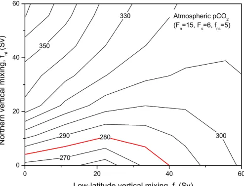
The sensitivity of modelled atmospheric pCO₂is illustrated in Figs. 2 and 3 (above) with

25

respect to variable mixing rates (f_{l i}, f_ns and f_ni), and in Figs. 4 and 5 with respect to 722

(14)

CPD

Full Screen / Esc

EGU

variable particle fluxes (P_s, P_l and P_n). Thus in Figs. 2 and 3 it is evident that modelled atmospheric pCO₂ is highly dependent on the magnitude of low latitude vertical mix-ing (f_{l i}) (i.e. stratification), moderately dependent on the mixing of intermediate- and North Atlantic water (f_ni) (i.e. intermediate-water up-welling in the North Atlantic), and essentially insensitive to the mixing of northern- and southern deep-water (f_ns).

5

Based on the results illustrated in Figs. 2 and 3 (and the expectation that f_nsfni<fl i)

the magnitudes of the mixing rates used for the Holocene model parameterisation have been estimated to yield modern atmospheric pCO₂∼280 ppm. It is notable that the viable range of values for f_{l i} is bi-modal and relatively narrow (either ∼5–10 or ∼30– 40 Sv), and that atmospheric pCO₂ is not particularly sensitive to f_ns. The northern

10

vertical mixing term, f_ni, essentially determines whether the low-latitude vertical mixing term, f_{l i}, should be high (∼30–40 Sv) or low (∼5–10 Sv). This means that modern at-mospheric pCO₂provides a strong constraint for setting the low-latitude vertical mixing (f_{l i}), in conjunction with the northern vertical mixing (f_ni) (assumed to be small relative to f_{l i}), while the deep mixing (f_ns) may be set freely so as to produce realistic contrasts

15

in the chemical composition (i.e. phosphate, alkalinity and TCO₂) of the various boxes it affects.

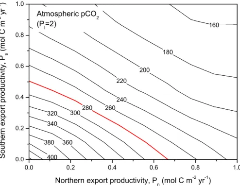
In Figs. 4 and 5, atmospheric pCO₂is shown to exhibit a strong sensitivity to chang-ing particle fluxes, and in particular to changes in the Southern Ocean export produc-tivity (P_s). This observation has two main implications: first, that large changes in pCO₂

20

may be efficiently obtained by arbitrarily changing the particle fluxes (as observed in previous box models); and second, that the modern pCO₂ provides a rigid constraint for the combined parameterisation of the model’s particle fluxes and vertical mixing rates (f_{l i} in particular). It is encouraging that the particle fluxes chosen on the basis of independent export productivity estimates (outlined above) can easily be made to

25

yield modern atmospheric pCO₂in conjunction with a reasonable and narrow range of vertical mixing rates.

(15)

CPD

Full Screen / Esc

EGU

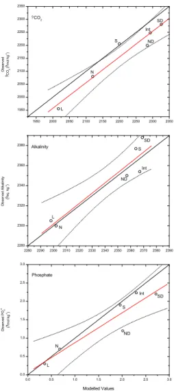
4.2 Model realism

The “skill” of the model in recreating modern conditions (given a choice of suitable parameters as outlined above) is illustrated in Fig. 6, where a comparison is made between modelled and observed estimates of phosphate, alkalinity and TCO₂for each box. Modern estimates for Atlantic chemistry have been drawn from Broecker and Peng

5

(1989) (based on the GEOSECS dataset) and from (Levitus, 1994). Although there is a tendency for the model to slightly overestimate the TCO₂ of all boxes (believed to be a result of using a global carbon budget in a purely “Atlantic” flow-scheme), and to significantly overestimate the phosphate of northern- and southern deep-water, the relationship between all modelled and modern values is satisfactory, and essentially

in-10

distinguishable from unity (at the 95% confidence interval). Of course, this comparison does not demonstrate that the box-model is a complete depiction of the global climate system. However, given that the main “tuning parameter” values have not been arbitrar-ily chosen, it does provide some confidence that the model design is realistic enough to be applied to an initial test of the “southern flavour” CO₂ sequestration hypothesis

15

outlined above.

5 Atmospheric pCO₂for a “southern flavour” ocean

5.1 The “hypsometric effect”

In Table 1, one of the input parameters is the volume ratio of northern- to southern sourced deep-water. This ratio has been calculated as being ∼8.9 today, on the

ba-20

sis of the Atlantic hypsometric curve (Menard and Smith, 1966), by assuming that North Atlantic sourced deep-water currently fills the depth interval ∼2–5 km, and that Antarctic-sourced water fills the abyssal Atlantic >5 km (McCartney, 1992). It is notable that the largest volumetric increment in the Atlantic is the 4–5 km section (closely fol-lowed by the 5–6 km section). This is illustrated in Fig. 7, where the volume ratio of two

25

(16)

CPD

Full Screen / Esc

EGU

water-masses that occupy horizontally stratified intervals in the deep Atlantic (>2 km) is plotted against the depth of the horizontal boundary between the two water-masses. This plot suggests that the water-mass that occupies more than the 4–5 km depth in-terval will essentially define the chemistry of the average deep marine reservoir, via a “hypsometric effect”.

5

5.2 Atmospheric CO₂linked to deep-water mass geometry and overturning

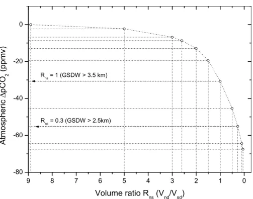
Figure 8 illustrates the effect of changing the relative volumes of the northern- and southern deep-water boxes in the model, expressed in terms of the ratio (R_ns) of northern- to southern deep-water box volumes, as defined in Fig. 7. As described above, the modern situation (North Atlantic deep-water filling the basin ∼2–5 km

10

depth) corresponds to R_ns∼8.9, while that inferred for the last glacial maximum, with southern-sourced deep-water filling the Atlantic basin up to 2.5 km depth, corresponds to R_ns∼0.3. When this value for Rns is used in the box model (with all other

parame-ters kept constant), CO₂ in the atmospheric box drops by ∼55 ppm (Fig. 8), which is equivalent to nearly 70% of the total glacial – interglacial CO₂change. The observed

15

“hypsometric effect” on carbon sequestration in the deep sea only becomes significant (and then increases rapidly) once the volumes of the southern and northern deep-water boxes are roughly equal. This would represent a situation where southern-sourced deep water has shoaled above ∼3.5 km water depth in the Atlantic. For a shoaling of southern sourced deep-water to only ∼3 km, CO₂ in the model drops by ∼45 ppm;

20

while for a near complete elimination of northern-sourced deep-water below 2 km water depth (i.e. a direct transfer of northern deep-water into the intermediate-depth ocean), CO₂drops by ∼68 ppm.

A significant “hypsometric” effect on atmospheric CO2 is thus confirmed in the box model, as suggested by the initial “southern flavour” thought experiment. However, as

25

found in previous box-model simulations, atmospheric CO₂ is also (indeed primarily) sensitive to the turnover rate of the ocean (in this case F_n and F_s), as well as the maximum “particle” export rate from the surface ocean. What this means is that

(17)

sig-CPD

Full Screen / Esc

EGU

nificant changes in carbon sequestration in the deep sea may be achieved by either changing the rate at which carbon in the deep-sea is “flushed out” by the overturning circulation and replenished by biological export (e.g. Sarmiento and Toggweiler, 1984; Toggweiler, 1999), or by filling the deep-sea with a particularly carbon-rich deep-water mass analogous to modern Antarctic Bottom Water (AABW), or by some additive

com-5

bination of these. A “target” glacial atmospheric CO₂ level of ∼200 ppm can therefore be easily reproduced in the box-model by using a variety of combinations of: 1) in-creased southern deep-water volume; 2) reduced overturning rates, of either southern (F_s) or northern (F_n) deep-water; and 3) increased particle export rates, especially in the Southern Ocean.

10

In previous box model investigations of marine carbon sequestration it was found that changes in the biological export of carbon to the deep sea or in the turnover rate of the ocean that were large enough to reproduce glacial atmospheric CO₂ levels, also tended to produce unrealistically dysoxic deep-waters (Toggweiler, 1999). In the box-model described here, a significant increase in the volume of southern sourced

15

deep-water allows this to be avoided (based on changes in phosphate concentration, southern/northern deep-water oxygenation levels drop/increase by ∼20%), primarily by decreasing the need to appeal to extreme changes in overturning- or biological export rates. This is illustrated in Fig. 9, where an increase in the budget of southern deep-water filling the box-model ocean is shown to reduce the need to invoke large changes

20

in ocean overturning or biological export in order to reproduce a glacial CO₂ levels. By filling the deep ocean with southern sourced deep-water, atmospheric CO₂ drops and becomes less sensitive to changes in the northern overturning cell, while also becoming more sensitive to biological export- and overturning circulation changes in the Southern Ocean. The carbon content of the deep ocean may thus become highly

25

dependent on its dominant overturning circulation route, as distinct from its overturning circulation rate.

In the real ocean, a large increase in the volume of southern-sourced deep-water ex-ported to the Atlantic and Indo-Pacific basins would require an increase in the amount

(18)

CPD

Full Screen / Esc

EGU

of water that has been converted from deep- and abyssal waters in the Southern Ocean (Orsi et al., 1999). This could be achieved via both thermohaline- and wind forcing; by: 1) increasing the density gradient between southern- and northern deep-water so as to stabilise the southern component over a broader density range of the deep ocean (Cox, 1989; Hughes and Weaver, 1994; Brix and Gerdes, 2003); and/or 2) reducing

5

the “Ekman suction” in the Southern Ocean by winding down the Antarctic Circumpolar Current (ACC), either via a reduced westerly wind stress (Toggweiler and Samuels, 1998), or via a reduced density gradient (and buoyancy flux) across this current (Cox, 1989; Karsten and Marshall, 2002). The mechanisms responsible for increasing the budget of deep-water exported northwards from deep within the ACC could therefore

10

closely overlap with those outlined by Watson and Naviera Garabato (2006) for reduc-ing the up-wellreduc-ing rate in the upper Southern Ocean (thus causreduc-ing deep- and intermedi-ate wintermedi-ater to be re-circulintermedi-ated internally instead). If, as proposed by Watson and Naviera Garabato (2006), this mechanism relied in part on an increase in the vertical density gradient in the Southern Ocean, this would also ensure that turbulent vertical diffusive

15

mixing (which may have been enhanced in a shallower glacial ocean (Wunsch, 2002)) would only serve to homogenise the deepest ocean carbon reservoir, without causing it to “leak” into the surface-ocean and atmosphere.

Note that the rate at which southern-sourced deep-water is exported need not in-crease in these scenarios as long as the standing volume of southern sourced

deep-20

water has stabilised. For a constant overturning rate of this (poorly “CO₂ ventilated”) southern sourced deep-sea reservoir, an increase in its volume equates to a propor-tionate increase in the residence time of carbon in that reservoir. Unless the rate of biological export of carbon from the surface ocean into this deep-sea reservoir de-creases significantly at the same time, this will necessitate a net increase in the amount

25

(19)

CPD

Full Screen / Esc

EGU

6 Closing the deficit of explained CO₂change

The main purpose of the present study is not to attempt a complete simulation or ex-planation of last glacial maximum atmospheric CO₂levels, but rather to investigate the plausibility and possible implications of a “hypsometric effect” on CO2 sequestration, which would arise due to large changes in the volume of southern-sourced deep-water

5

filling the ocean basins. The “southern flavour ocean” theory proposed here has the advantage of being relatively parsimonious in its premises (i.e. it requires few changes to the ocean system in order to operate), and of being based on premises that should be easily refutable by proxy evidence, yet nonetheless are well supported by available data and modelling studies (Duplessy et al., 1988; Michel et al., 1995; Rutberg et al.,

10

2000; Kim et al., 2003; Shin et al., 2003; Piotrowski et al., 2004, 2005; Curry and Oppo, 2005). Furthermore, the proposed changes in the volumetric dominance of southern-sourced deep-water might be expected to be controlled by its density, and therefore to vary inversely to changes in its temperature. This may suggest a mechanism that could explain the proposed links between atmospheric CO₂ and those components of

15

the deep-water temperature and global ice-volume records that cannot be explained by linear insolation forcing (Shackleton, 2000; Parrenin and Paillard, 2003).

It is worth noting that the operation of the hypsometric effect in the box-model de-scribed here is not primarily dependent on an exaggeration of the efficiency of gas exchange at high latitudes (Archer et al., 2000a; Toggweiler et al., 2003a, b) since it

20

operates via changes in the relative magnitudes of different intra-oceanic carbon reser-voirs, rather than changes in their extent of equilibration with the atmosphere. Indeed, the hypothesis proposed here essentially functions through an expansion of a “glacial analogue of AABW” to the majority of the deep ocean. What the proposed mechanism does require is that glacial deep-water formation in the southern ocean operated in a

25

broadly similar fashion to today, with a significant amount of water-mass conversion occurring away from the air-sea interface, and that vertical diffusivity was not so large (Archer et al., 2000a, b), or could not operate so efficiently against density gradients in

(20)

CPD

Full Screen / Esc

EGU

the glacial ocean, that it was able to erode vertical gradients in carbon content more ef-ficiently than they could be replaced by the physical and biological export mechanisms posited here.

Further studies, using more complete and complex model simulations, will be re-quired in order to determine more securely the veracity and magnitude of the proposed

5

hypsometric effect. Nevertheless, if this simple mechanism for enhancing deep-sea carbon sequestration is incorporated explicitly into the list of “ingredients” that have contributed to glacial – interglacial CO₂ change (Archer et al., 2000b; Sigman and Boyle, 2000), it may help to reduce the “CO₂ deficit” that remains to be explained by appealing to more “extreme” or controversial processes. Although, as previously, the

10

mystery of glacial – interglacial CO₂change still eludes us (Archer et al., 2000b), per-haps it is not quite as distant as we might have believed?

Acknowledgements. This work was enabled by a Research Fellowship held by the author at

Christ’s College, at the University of Cambridge. The author is very grateful for interesting discussions with D. Paillard, T. Stocker and A. Timmermann. The author is particularly grateful

15

for helpful and insightful discussions with E. Gloor, as well as his comments on an initial version of this manuscript.

References

Archer, D., Eshel, G., Winguth, A., Broecker, W. S., Pierrehumbert, R., Tobis, M., and Jacob, R.: Atmospheric pCO₂ sensitivity to the bioloical pump in the ocean, Global Biochem. Cycles,

20

14, 1219–1230, 2000a.

Archer, D. and Maier-Reimer, E.: Effect of deep-sea sedimentary calcite preservation on atmo-spheric CO2 concentration, Nature, 367, 260–263, 1994.

Archer, D., Winguth, A., Lea, D. W., and Mahowald, N.: What caused the glacial/interglacial atmospheric pCO₂cycles?, Rev. Geophys., 38, 159–189, 2000b.

25

Bard, E.: Correction of accelerator mass spectrometry 14C ages measured in planktonic foraminifera: Paleoceanographic implications, Paleoceanography, 3, 635–645, 1988.

(21)

CPD

Full Screen / Esc

EGU

Boyle, E.: Cadmium and d13C paleochemical ocean distributions during the Stage 2 glacial maximum, Ann. Rev. Earth Planet. Sci., 20, 245–287, 1992.

Boyle, E. A.: The role of vertical fractionation in controlling late Quaternary atmospheric carbon dioxide, J. Geophys. Res., 93, 15 701–15 714, 1988.

Brix, H. and Gerdes, R.: North Atlantic Deep Water and Antarctic Bottom Water: Their

in-5

teraction and influence on the variability of the global ocean circulation, J. Geophys. Res., 108(C2), doi:10.1029-2002JC0021335, 2003.

Broecker, W.: How strong is the Harvardton-Bear constraint?, Global Biogeochem. Cycles, 13, 817–820, 1999.

Broecker, W. S.: Glacial to interglacial changes in ocean chemistry, Progress in Oceanography,

10

11, 151–197, 1982a.

Broecker, W. S.: Ocean chemistry during glacial time, Geochim. Cosomochim. Acta, 46, 1698– 1705, 1982b.

Broecker, W. S. and Peng, T.-H.: The cause of the glacial to interglacial atmospheric CO2 change: a polar alkalinity hypothesis, Global Biogeochem. Cycles, 3, 215–239, 1989.

15

Chester, R.: Marine Geochemistry, Blackwell, Oxford, 2003.

Cox, M. D.: An idealized model of the world ocean. Part I: The global-scale water masses, J. Phys. Oceanogr., 19, 1730–1752, 1989.

Curry, W. B., Duplessy, J. C., Labeyrie, L. D., and Shackleton, N. J.: Changes in the distri-bution of d13C of deep water sigma-CO2 between the last glaciation and the Holocene,

20

Paleoceanography, 3, 317–341, 1988.

Curry, W. B. and Oppo, D. W.: Glacial water mass geometry and the distribution of d13C of Sigma-CO2 in the western Atlantic Ocean, Paleoceanography, 20, PA1017, doi:10.1029/2004PA001021, 2005.

Duplessy, J.-C., Shackleton, N. J., Fairbanks, R. G., Labeyrie, L., Oppo, D., and Kallel, N.:

25

Deep water source variations during the last climatic cycle and their impact on global deep water circulation, Paleoceanography, 3, 343–360, 1988.

Ganachaud, A. and Wunsch, C.: Improved estimates of global ocean circulation, heat transport and mixing from hydrographic data, Nature, 408, 453–457, 2000.

Gildor, H. and Tziperman, E.: Physical mechanisms behind biogeochemical glacial-interglacial

30

CO₂variations, Geophys. Res. Lett., 28, 2421–2424, 2001.

Hughes, T. M. C. and Weaver, A. J.: Multiple Equilibria of an Asymmetric Two-Basin Ocean Model, J. Phys. Oceanogr., 28, 619–637, 1994.

(22)

CPD

Full Screen / Esc

EGU

Karsten, R. H. and Marshall, J.: Testing theories of the vertical stratification of the ACC against observations, Dynamics of Atmospheres and Oceans, 36, 233–246, 2002.

Keeling, R. F. and Stephens, B. B.: Antarctic sea ice and the control of Pleistocene climate instability, Paleoceanography, 16, 112–131, 2001.

Keigwin, L. D.: Radiocarbon and stable isotope constraints on Last Glacial Maximum and

5

Younger Dryas ventilation in the western North Atlantic, Paleoceanography, 19, 1–15, 2004. Keigwin, L. D. and Lehmann, S. J.: Deep circulation change linked to Heinrich event 1 and

Younger Dryas in a mid-depth North Atlantic core, Paleoceanography, 9, 185–194, 1994. Kim, S.-J., Flato, G. M., and Boer, G. J.: A coupled climate model simulation of the Last Glacial

Maximum, Part 2: approach to equilibrium, Clim. Dyn., 20, 635–661, 2003.

10

Knox, F. and McElroy, M.: Changes in atmospheric CO2: influence of marine biota at high latitude, J. Geophys. Res., 89, 4629–4637, 1984.

Levitus, S.: World Ocean Atlas, NOAA, Washington D.C., 1994.

Longhurst, A., Sathyendranath, S., Platt, T., and Caverhill, C.: An estimate of global primary production in the ocean from satellite radiometer data, J. Plankton Res., 17, 1245–1271,

15

1995.

Marchitto, T. M., Oppo, D. W., and Curry, W. B.: Paired benthic foraminiferal Cd/Ca and Zn/Ca evidence for a greatly increased presence of Southern Ocean Water in the glacial North Atlantic, Paleoceanography, 17, 10.1–10.16, 2000PA000598, 2002.

Martin, J. H., Knauer, G. A., Karl, D. M., and Broenkow, W. W.: VERTEX: carbon cycling in the

20

northeast Pacific, Deep Sea Res., 34, 267–286, 1987.

McCartney, M. S.: Recirculating components to the deep boundary current of the northern North Atlantic, Progress in Oceanography, 29, 283–383, 1992.

Menard, H. W. and Smith, S. M.: Hypsometry of ocean basin provinces, J. Geophys. Res., 71, 4305–4325, 1966.

25

Michel, E., Labeyrie, L., Duplessy, J.-C., and Gorfti, N.: Could deep Subantarctic convection feed the worl deep basins during last glacial maximum?, Paleoceanography, 10, 927–942, 1995.

Naviera Garabato, A. C., Polzin, K. L., King, B. A., Heywood, K. J., and Visbeck, M.: Widespread intense turbulent mixing in the Southern Ocean, Science, 303, 210–213, 2004.

30

Oppo, D. and Fairbanks, R. G.: Atlantic ocean thermohaline circulation of the last 150 000 years: Relationship to climate and atmospheric CO2, Paleoceanography, 5, 277–288, 1990. Oppo, D. W., Fairbanks, R. G., Gordon, A. L., and Shackleton, N. J.: Late Pleistocene Southern

(23)

CPD

Full Screen / Esc

EGU

Ocean d13C variability, Paleoceanography, 5, 43–54, 1990.

Orsi, A. H., Johnson, G. C., and Bullister, J. L.: Circulation, mixing and production of Antarctic Bottom Water, Progress in Oceanography, 43, 55–109, 1999.

Parrenin, F. and Paillard, D.: Amplitude and phase of glacial cycles from a conceptual model, Earth Planet. Sci. Lett., 214, 243–250, 2003.

5

Piotrowski, A., Goldstein, S. L., Hemming, S. R., and Fairbanks, R. G.: Temporal relationships of carbon cycling and ocean circulation at glacial boundaries, Science, 307, 1933–1938, 2005.

Piotrowski, A. M., Goldstein, S. L., Hemming, S. R., and Fairbanks, R. G.: Intensification and variability of ocean thermohaline circulation through the last deglaciation, Earth Planet. Sci.

10

Lett., 225, 205–220, 2004.

Robinson, L. F., Adkins, J. F., Keigwin, L. D., Southon, J., Fernandez, D. P., Wang, S.-L., and Scheirer, D. S.: Radiocarbon variability in the western North Atlantic during the last deglaciation, Science, 310, 1469–1473, 2005.

Rutberg, R. L., Heming, S. R., and Goldstein, S. L.: Reduced North Atlantic Deep Water flux to

15

the glacial Southern Ocean inferred from neodymium isotope ratios, Nature, 405, 935–938, 2000.

Sabine, C., Feely, R. A., Gruber, N., Key, R. M., Lee, K., Bullister, J. L., Wanninkhof, R., Wong, C. S., Wallace, D. W. R., Tilbrook, B., Millero, F. J., Peng, T.-H., Kozyr, A., Ono, T., and Rios, A. F.: The oceanic sink for anthropogenic CO2, Science, 305, 367–371, 2004.

20

Santos, V., Billett, D. S. M., Rice, A. L., and Wolff, G. A.: Organic matter in deep-sea sediments from the Porcupine Abyssal Plain in the northeast Atlantic Ocean. I – Lipids, Deep Sea Res., 41, 787–819, 1994.

Sarmiento, J. L. and Toggweiler, R.: A new model for the role of the oceans in determining atmospheric pCO2, Nature, 308, 621–624, 1984.

25

Shackleton, N. J.: The 100 000-year ice-age cycle identified and found to lag temperature, carbon dioxide and orbital eccentricity, Science, 289, 1897–1902, 2000.

Shin, S. I., Liu, Z., Otto-Bliesner, B. L., Brady, E. C., Kutzbach, J. E., and Harrison, S. P.: A simulation of the last glacial maximumclimate using the NCAR-CCSM, Clim. Dyn., 20, 127– 151, 2003.

30

Siegenthaler, U., Stocker, T. F., Monnin, E., Luthi, D., Schwander, J., Stauffer, B., Raynaud, D., Barnola, J.-M., Fischer, H., Masson-Delmotte, V., and Jouzel, J.: Stable carbon cycle – climate relationship during the Late Pleistocene, Science, 310, 1313–1317, 2005.

(24)

CPD

Full Screen / Esc

EGU

Siegenthaler, U. and Wenk, T.: Rapid atmospheric CO2 variations and ocean circulation, Na-ture, 308, 624–625, 1984.

Sigman, D. M. and Boyle, E. A.: Glacial/interglacial variations in atmospheric carbon dioxide, Nature, 407, 859–869, 2000.

Skinner, L. C. and Shackleton, N. J.: Rapid transient changes in Northeast

At-5

lantic deep-water ventilation-age across Termination I, Paleoceanography, 19, 1–11, doi:10.1029/2003PA000983, 2004.

Speer, K., Rintoul, S. R., and Sloyan, B.: The diabatic deacon cell, J. Phys. Oceanogr., 30, 3212–3222, 2000.

Toggweiler, J. R.: Variation of atmospheric CO2 by ventilation of the ocean’s deepest water,

10

Paleoceanography, 14, 571–588, 1999.

Toggweiler, J. R., Gnanadesikan, A., Carson, S., Murnane, R., and Sarmiento, J. L.: Represen-tation of the carbon cycle in box models and GCMs: 1. Solubility pump, Global Biogechem. Cycles, 17, 26.1–26.11, doi:10.1029/2001GB001401, 2003a.

Toggweiler, J. R., Murnane, R., Carson, S., Gnanadesikan, A., and Sarmiento, J. L.:

Represen-15

tation of the carbon cycle in box models and GCMs: 2. Organic pump, Global Biogeochem. Cycles, 17, 27.1–27.13, doi:10.1029/2001GB001841, 2003b.

Toggweiler, J. R. and Samuels, B.: On the Ocean’s Large-Scale Circulation near the Limit of No Vertical Mixing, J. Phys. Oceanogr., 28, 1832–1852, 1998.

Toggweiler, J. R. and Sarmiento, J. L.: Glacial to interglacial changes in atmospheric carbon

20

dioxide: the critical role of ocean surface water in high latitudes, in: The Carbon Cycle and At-mospheric CO2: Natural Variations Archean to Present, pp. 163–184, Geophys. Monograph, American Geophysical Union, 1985.

Watson, A. J. and Naveira Garabato, A. C.: The role of Southern Ocean mixing and upwelling in glacial – interglacial atmospheric CO2 change, Tellus 58B, 73–87, 2006.

25

Webb, D. J. and Suginohara, N.: Vertical mixing in the ocean, Nature, 409, 37, 2001. Wunsch, C.: What is the thermohaline circulation?, Science, 298, 1179–1181, 2002.

(25)

CPD

Full Screen / Esc

EGU

Table 1. Input parameterisation for modern model scenario.

Parameter Parameter label Value Parameter Parameter label Values Fluxes Temperature, salinity

Northern overturning Fn 15 Sv Southern temperature Ts 5

◦

C Southern overturning Fs 6 Sv Low lat. temperature Tl 21.5

◦

C Low lat. vertical mixing fl i 35 Sv Northern temperature Tn 8

◦

C Northern vertical mixing fni 8 Sv Southern salinity Ss 34.7‰

Deep mixing fns 5 Sv Low lat. salinity Sl 36.0

Gas exchange – south Gs 5 m day

−1

Northern salinity Sn 35.0‰

Gas exchange – low lat. Gl 3 m day

−1

Particle fluxes Gas exchange – north Gn 5 m day

−1

Southern export Ps 0.2 mol Cm

−2

yr−1 Volumes, areas Low lat. export Pl 2.0 mol Cm

−2

yr−1 Total volume ocean Vo 1.3×10

18

m3 Northern export Pn 0.4 mol Cm

−2

yr−1 Total area ocean Ao 3.5×10

14

m3 Redfield ratios

Volume atmosphere Vatm 1.773×1020moles Carbon/phosphorus C/P 106

N. Atlantic area/total area An/Ao 0.2 Nitrogen/phosphorus N/P 16

S. Atlantic area/total area As/Ao 0.35 Southern CaCO3/TCO2 S-CaCO3/CO2 0.10

Vol. NADW/Vol. AABW RVns 0.5 Low lat. CaCO3/TCO2 L-CaCO3/CO2 0.20

Global masses Northern CaCO3/TCO2 N-CaCO3/CO2 0.25

Total phosphate Pglob 2.769×10 15

mol Total alkalinity Aglob 3.14×1018mol

Total CO2 TCO2glob 3.0379×10 18

mol

(26)

CPD

Full Screen / Esc

Printer-friendly Version Interactive Discussion EGU P s S Int SD L N S ND F s F n (F s +F n ) P n P l f(P l ) f(P l ) (1-f)(P l ) f ni f ns f li Atmosphere G s G l Gs G n

Fig. 1. Box-model schematic (S, southern surface; L, low-latitude surface; N, northern surface; ND, north deep; Int, intermediate; SD, south deep). Heavy black lines indicate thermohaline circulation (Fn = northern overturning; Fs = southern overturning). Red arrows indicate

two-way exchange (i.e. mixing) terms. Blue arrows indicate gas exchange. Grey arrows indicate particle fluxes. The particle fluxes to the deep boxes are partitioned according to the relative volumes of the ND and SD boxes (see text).

(27)

CPD

Full Screen / Esc

Printer-friendly Version Interactive Discussion EGU 270 280 290 300 330 340 350 0 20 40 60 0 20 40 60 Atmospheric pCO 2 (F n =15, F s =6, f ns =5) N o r t h e r n v e r t i ca l m i x i n g , f n i ( S v )

Low-latitude vertical mixing, f li

(Sv)

Fig. 2. Sensitivity of modelled atmospheric pCO₂(µatm) to variable low-latitude (fl i) and

north-ern (fni) vertical mixing rates. Other model parameters are as listed in Table 1.

(28)

CPD

Full Screen / Esc

Printer-friendly Version Interactive Discussion EGU 285 280 275 275 280 285 290 295 300 0 10 20 30 40 50 60 70 80 0 10 20 30 40 50 60 70 80 Atmospheric pCO 2 (F n =15, F s =6, f ni =8) L o w -l a t i t u d e v e r t i ca l m i x i n g , f l i ( S v )

Deep north-south mixing, f ns

(Sv)

Fig. 3. Sensitivity of modelled atmospheric pCO₂ (µatm) to low-latitude (fl i) and deep (fns)

(29)

CPD

Full Screen / Esc

Printer-friendly Version Interactive Discussion EGU 0.0 0.5 1.0 1.5 2.0 150 200 250 300 350 400 450 500 Modern pCO 2 A t m o sp h e r i c p C O 2 ( a t m )

Export flux (molC m -2 yr -1 ) P l (P n =0.4, P s =0.2) P n (P l =2, P s =0.2) P s (P l =2, P n =0.4)

Fig. 4. Sensitivity of modelled atmospheric pCO₂ (µatm) to variable particle export fluxes (North Atlantic, Pn; South Atlantic, Ps; Low-latitude, Pl). Other model parameters are as listed

in Table 1.

(30)

CPD

Full Screen / Esc

Printer-friendly Version Interactive Discussion EGU 400 380 360 340 320 300 280 260 240 220 200 180 160 0.0 0.2 0.4 0.6 0.8 1.0 0.0 0.2 0.4 0.6 0.8 1.0 Atmospheric pCO 2 (P l =2) S o u t h e r n e x p o r t p r o d u ct i v i t y , P s ( m o l C m -2 y r -1 )

Northern export productivity, P n (mol C m -2 yr -1 )

Fig. 5. Sensitivity of modelled atmospheric pCO₂ (µatm) to variable northern- and southern particle fluxes. Other model parameters are as listed in Table 1.

(31)

CPD

Full Screen / Esc

Printer-friendly Version Interactive Discussion EGU 0.0 0.5 1.0 1.5 2.0 2.5 3.0 0.0 0.5 1.0 1.5 2.0 2.5 3.0 S SD Int ND N L Phos phate O b se r ve d P O 4 2-( m o l kg -1 ) Modelled Values 2280 2290 2300 2310 2320 2330 2340 2350 2360 2370 2380 2390 2280 2300 2320 2340 2360 2380 L N S ND Int SD Alkalinity O b se rve d A lka lin ity ( e q . kg -1) 1950 2000 2050 2100 2150 2200 2250 2300 2350 1950 2000 2050 2100 2150 2200 2250 2300 2350 L N ND SD Int S CO 2 O b se r ve d C O 2 ( m o l kg -1 )

Fig. 6. Model skill, for mod-ern reconstruction of phosphate, alkalinity and total dissolved CO2 (ΣCO2). Data labels

in-dicate boxes: L, Low-latitude surface; N, North surface; S, South surface; Int, Intermedi-ate; ND, North deep; SD, South deep. Model parameters are listed in Table 1. Solid red lines and dotted black lines indicate least squares regression onto the data and 95% confidence in-tervals respectively. Solid black lines indicate 1:1 relationship. 740

(32)

CPD

Full Screen / Esc

Printer-friendly Version Interactive Discussion EGU 1 2 3 4 5 0 1 2 3 4 5 6 7 8 9 10 4-5 km section ~ 77 % change in V nd /V sd R n s = V n d w / V s d w Base of NADW (km)

Fig. 7. Volume ratio of northern (upper) deep-water to southern (lower) deep-water plotted against the depth of the base of the upper deep-water layer, as defined by the hypsometry of the Atlantic basin (Menard and Smith, 1966).

(33)

CPD

Full Screen / Esc

Printer-friendly Version Interactive Discussion EGU 9 8 7 6 5 4 3 2 1 0 -80 -60 -40 -20 0 R ns = 1 (GSDW > 3.5 k m) R ns = 0.3 (GSDW > 2.5k m) A t m o sp h e r i c p C O 2 ( p p m v ) Volume ratio R ns (V nd /V sd )

Fig. 8. Simulated changes in atmospheric CO₂, with respect to modern (280 ppm) caused by varying the ratio of northern- to southern sourced deep-water (Vn/Vs) filling the Atlantic. GSDW

refers to “glacial southern sourced deep water”, the glacial analogue for modern AABW.

(34)

CPD

Full Screen / Esc

Printer-friendly Version Interactive Discussion EGU 0.2 0.4 0.6 0.8 1.0 -140 -120 -100 -80 -60 -40 -20 0

Maximum southern export productiv ity, P s (mol C m -2 yr -1 ) 14 12 10 8 6 4 2 0 -140 -120 -100 -80 -60 -40 -20 0 20 Ch a n g e f r o m m o d e r n CO 2 ( p p m ) Northern ov erturning, F n (Sv ) 16 14 12 10 8 6 4 2 0 -120 -100 -80 -60 -40 -20 0 20 40 60 R ns = 8.9 (GSDW >5km) Rns= 1.0 (GSDW >4km) R ns = 0.27 (GSDW >2.5km) Southern overturning, F s (Sv)

Fig. 9. Changes in atmospheric CO₂, from modern (280 ppm), produced in the box-model for different volume ratios of northern- versus southern deep-water (Rns), in conjunction with: 1)

changes in southern overturning; 2) changes in northern overturning; and 3) changes in the maximum level of southern ocean export productivity.