HAL Id: hal-00318388
https://hal.archives-ouvertes.fr/hal-00318388
Submitted on 2 Oct 2007
HAL is a multi-disciplinary open access
archive for the deposit and dissemination of
sci-entific research documents, whether they are
pub-lished or not. The documents may come from
teaching and research institutions in France or
abroad, or from public or private research centers.
L’archive ouverte pluridisciplinaire HAL, est
destinée au dépôt et à la diffusion de documents
scientifiques de niveau recherche, publiés ou non,
émanant des établissements d’enseignement et de
recherche français ou étrangers, des laboratoires
publics ou privés.
Origin of temperature anisotropies in the cold plasma
sheet: Geotail observations around the
Kelvin-Helmholtz vortices
M. N. Nishino, M. Fujimoto, G. Ueno, T. Mukai, Y. Saito
To cite this version:
M. N. Nishino, M. Fujimoto, G. Ueno, T. Mukai, Y. Saito. Origin of temperature anisotropies in the
cold plasma sheet: Geotail observations around the Kelvin-Helmholtz vortices. Annales Geophysicae,
European Geosciences Union, 2007, 25 (9), pp.2069-2086. �hal-00318388�
www.ann-geophys.net/25/2069/2007/ © European Geosciences Union 2007
Annales
Geophysicae
Origin of temperature anisotropies in the cold plasma sheet: Geotail
observations around the Kelvin-Helmholtz vortices
M. N. Nishino1,2, M. Fujimoto2, G. Ueno3, T. Mukai4, and Y. Saito2
1School of Science, The University of Tokyo, Tokyo 113-0033, Japan 2ISAS/JAXA, Kanagawa 229-8510, Japan
3Institute of Statistical Mathematics, Tokyo 106-8569, Japan 4JAXA, Tokyo 100-8260, Japan
Received: 19 June 2007 – Revised: 13 September 2007 – Accepted: 18 September 2007 – Published: 2 October 2007
Abstract. To further our understanding of the solar wind en-try across the magnetopause under northward IMF, we per-form a case study of a duskside Kelvin-Helmholtz (KH) vor-tex event on 24 March 1995. We have found that the pro-tons consist of two separate (cold and hot) components in the magnetosphere-like region inside the KH vortical struc-ture. The cold proton component occasionally consisted of counter-streaming beams near the current layer in the KH vortical structure. Low-energy bidirectional electron beams or flat-topped electron distribution functions in the direction along the local magnetic field were apparent on the magneto-sphere side of the current layer. We discuss that the bidirec-tionality of the electrons and the cold proton component im-plies magnetic reconnection inside the KH vortical structure. In addition, we suggest selective heating of electrons inside the vortical structure via wave-particle interactions. Com-paring temperatures in the magnetosphere-like region inside the vortical structure with those in the cold plasma sheet, we show that further heating of both the electrons and the cold proton component is taking place in the cold plasma sheet or on the way from the vortices to the cold plasma sheet. Keywords. Magnetospheric physics (Magnetotail; Magne-totail boundary layers; Plasma sheet)
1 Introduction
The plasma sheet in the near-Earth magnetosphere be-comes cold under the northward interplanetary magnetic field (IMF) (e.g. Zwolakowska et al., 1992; Zwolakowska and Popielawska, 1992; Terasawa et al., 1997; Borovsky et al., 1998; Nishino et al., 2002; Wing et al., 2005). Such cold plasma is thought to be of solar wind origin and to come into the near-Earth plasma sheet through the low-latitude
Correspondence to: M. N. Nishino
(nishino@stp.isas.jaxa.jp)
boundary layer (LLBL) in the tail-flank regions (e.g. Tera-sawa et al., 1997; Fujimoto et al., 1998). The entry mecha-nism of the solar wind plasma under northward IMF is still under debate.
As candidates for entry mechanism of the solar wind plasma under northward IMF, double high-latitude reconnec-tion on the dayside and Kelvin-Helmholtz (KH) instability in the tail flanks have been proposed. Double high-latitude reconnection has been thought to take place under strongly northward IMF (Song and Russell, 1992; Li et al., 2005; Øieroset et al., 2005), and in-situ evidence of this process was found by recent satellite observations (Onsager et al., 2001; Lavraud et al., 2005, 2006). The KH instability is ex-pected to occur in the flank regions because of velocity shear across the magnetopause (Fairfield et al., 2000). Simulations (Otto and Fairfield, 2000; Nykyri and Otto, 2001; Matsumoto and Hoshino, 2006; Nakamura et al., 2006), as well as obser-vational studies (e.g. Hasegawa et al., 2004, 2006) have sug-gested a development of the vortical structure under strongly northward IMF. Furthermore, simulation studies (e.g. Otto and Fairfield, 2000; Nykyri and Otto, 2001; Nakamura et al., 2006) suggested that magnetic reconnection may occur in the KH vortices and that it can play an important role in plasma transport across the magnetopause. A recent observational study by Nykyri et al. (2006) suggested reconnection signa-tures in the flank region on the dawnside associated with KH instability, although the IMF did not point strongly north-ward in their event.
In the cold plasma sheet and the LLBL, the electrons fre-quently have a parallel anisotropy where parallel tempera-ture dominates over the perpendicular one (Hada et al., 1981; Traver et al., 1991; Phan et al., 1997; Fujimoto et al., 1998). The parallel anisotropy of low energy protons in the dusk flank plasma sheet has also been pointed out by Traver et al. (1991) and Nishino et al. (2007a). A recent study by Nishino et al. (2007b) showed that strong parallel anisotropies of both the electrons and the cold proton component occur under
strongly northward IMF, and suggested that the anisotropies may be related to the rolled-up KH vortices in the tail flank. Nishino et al. (2007b) also found that the low-energy por-tion of the electron distribupor-tion funcpor-tions in the cold plasma sheet has a flat-topped shape, and that the parallel anisotropy of electrons is stronger than that of the cold proton com-ponent, which implies that some other mechanism, such as wave-particle interactions, works besides adiabatic heating.
In order to study strong parallel anisotropies around the KH vortices under strongly northward IMF, we focus on the duskside magnetopause crossing event on 24 March 1995. During this day strongly northward IMF was monitored by upstream Wind for a prolonged interval, and the Geotail spacecraft observed quasi-periodic wavy structures around the LLBL on the duskside (Fujimoto et al., 1998). Fairfield et al. (2000) suggested that the wavy structures are due to the development of KH vortices, with the support of sim-ulations by Otto and Fairfield (2000) that proposed the oc-currence of magnetic reconnection in the KH vortical struc-tures. Furthermore, the magnetopause has been shown to be rolled-up at times due to the KH instability, as demonstrated in an observational study by Hasegawa et al. (2006). In the cold plasma sheet adjacent to the LLBL, the ions consisted of two separate components, which showed spatial admix-ture of the solar wind ions and the magnetospheric hot ions (Fujimoto et al., 1998). The low-energy portion of the elec-trons on the magnetosphere side around the boundary had a parallel (bidirectional) anisotropy along the magnetic field (Fujimoto et al., 1998; Fairfield et al., 2000). Nishino et al. (2007b) reported that both the electrons and the cold pro-ton component in the cold plasma sheet had strong parallel anisotropies in this event. A detailed study of distribution functions, in addition to temperature anisotropies around the KH vortical structures, will provide more information about the physical mechanism which has impacted the plasmas dur-ing the cold plasma sheet formation. We examine tempera-ture anisotropies of electrons and protons inside the KH vor-tical structures, as well as inspect the velocity distribution functions in detail, comparing them with those in the cold plasma sheet.
2 Instrumentation
We use data from the three-dimensional (3-D) electron and ion distribution functions obtained every 12 s by the low energy particle (Geotail/LEP) experiment (Mukai et al., 1994). The magnetic field data are obtained every 1/16 s by the flux-gate magnetometer (Geotail/MGF) (Kokubun et al., 1994). The electrons are detected by the electron analyzer of LEP-EAe, and we use data of the low-energy mode in the range between 8.3 eV and 7.6 keV. The ion energy-per-charge analyzer of LEP-EAi detects ions between 32 eV/q and 39 keV/q, which covers most of the typical energy range of protons in the boundary layer and the cold plasma sheet.
In the present study, all of the detected positively-charged ions are assumed to be protons. Solar wind parameters ob-tained by the Wind spacecraft were provided via CDAWeb. The Wind data are from SWE (Ogilvie et al., 1995) and MFI (Lepping et al., 1995). We use the GSM coordinate system throughout the paper.
3 Calculation of moment parameters
For electrons, we obtain effective temperatures in the per-pendicular and parallel directions to the local magnetic field, which are denoted as Te⊥and Tek, respectively. Although the
typical kinetic energy of photoelectrons is less than the elec-tric potential of the spacecraft, which is lower than 10 eV in the cold plasma sheet (Ishisaka et al., 2001), some photoelec-trons have energy higher than the spacecraft potential (Ueno et al., 2001b). We therefore checked the observed electron distribution functions, and utilize PSDs with energy higher than 12.86 eV to exclude photoelectrons.
For protons, we not only calculate moment parameters by simple moment calculations but also deal with cold and hot components separately, for the data where two components are apparent. To separate the ion distribution function into the cold and hot components, we utilize a two-Maxwellian mixture model with a scheme developed by Ueno et al. (2001a), as Nishino et al. (2007a) performed. Perpendicu-lar and parallel temperatures of the cold and hot components are denoted as TC⊥, TCk, TH⊥, and THk, respectively. Proton
temperatures from the simple moment calculations are rep-resented by Tp⊥and Tpk.
4 Observations 4.1 Overview
Figure 1 shows the solar wind observations between 00:00– 10:00 UT on 24 March 1995. From the top, (a) latitudi-nal angle of the IMF (θIMF), (b) strength (black line), Y (green) and Z (red) components of the IMF, (c) proton den-sity, and (d) bulk flow speed are presented. The IMF pointed strongly northward (θIMF>45◦) and the density was higher than 10 cm−3throughout the interval. The bulk flow speed was as slow as 330–340 km/s. The convection time of the so-lar wind from the Wind location (X∼219 RE) to the Earth’s
magnetosphere, which is not included in the figure, was about 70 min.
Figure 2 shows the projection onto the GSM-XY plane of the Geotail orbit between 06:50–10:00 UT. The space-craft gradually moved toward the midnight region with its
Zcoordinate decreasing from 3.9 REto 1.9 RE(not shown).
Figure 3 shows an overview of the Geotail observations for the interval. From the top, (a–b) energy-time (E-t) spec-trograms of omni-directional electrons and ions, (c) elec-tron temperatures in the direction perpendicular (green) and
(a)
(c)
(d)
Solar wind observations (Wind)
10:00 00:00 02:00 04:00 06:00 08:00 (UT) IM F la t. (cm -3) d en si ty b ul k sp ee d (d eg ) (b) B (nT) (k m /s ) 0 100 200 300 400 500 00:00-10:00 UT 24 March 1995 -10-5 0 5 10 15 0 10 20 30 |B| By Bz -90 -45 0 45 90
Fig. 1. Solar wind observations by Wind (X∼219 RE) between
00:00–10:00 UT on 24 March 1995. From the top, (a) the latitudi-nal angle of the IMF, (b) strength (black), Y (green), and Z (red) components of the IMF, (c) proton density, and (d) bulk flow speed
are presented. The convection time (∼70 min) is not included in the
figure.
parallel (blue) to the local magnetic field, (d) proton tem-peratures, (e) VX (blue) and VY (green) of bulk proton ve-locity, and (f) three components of the magnetic field are presented. Locations of the Geotail spacecraft are given at the bottom of the figure. Large perturbations in the mag-netic field, the velocity, and the electron and proton tem-peratures are attributed to encounters with the vortical struc-tures of the KH instability around the boundary. Concern-ing the inbound transition of the Geotail spacecraft from the magnetosheath to the plasma sheet, Fairfield et al. (2000) categorized the observed data into four separate regions: the magnetosheath (until 03:54 UT, not shown here), the exterior interaction region (between 03:54–07:16 UT), the interior interaction region (between 07:16–09:10 UT), and the cold plasma sheet (after 09:11 UT). In the interior in-teraction region Geotail observed magnetosheath-like dense plasma and magnetosphere-like plasma alternately with a quasi-period of about 3–5 min. By a visual inspection of the data shown in Fig. 3, we have found that around 08:00 UT the bulk flow speed slowed down, fluctuations in the mag-netic field reduced, and magnetosphere-like plasma was ob-served for several minutes. In order to examine the transi-tion of plasma from the dense magnetosheath-like region to the stagnant magnetosphere-like region, we study the data around 08:00 UT in more detail.
-20 -10 0 10 20 -30 -20 -10 0 10
Y
GSM(R
e)
X
GSM(R
e)
Geotail orbit (GSM)
06:50-10:00 UT 24 March 1995
06:50 UT 10:00 UTFig. 2. Projection onto the GSM-XY plane of the Geotail orbit between 06:50–10:00 UT on 24 March 1995. A dotted curve in the figure corresponds to the averaged location of the magnetopause calculated with a model by Roelof and Sibeck (1993).
4.2 Categorization of regions inside vortices
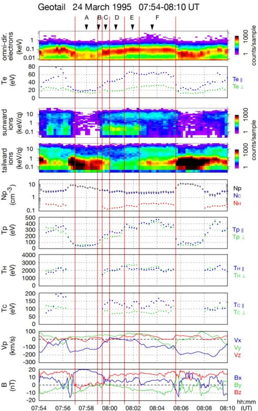
In Fig. 4 we expand the Geotail observation for the 16-min interval 07:54–08:10 UT during which the satellite repeated multiple crossings of the boundary. From the top, E-t spec-trogram of omni-directional electrons, electron temperatures, E-t spectrograms of sunward and tailward ions, ion densi-ties, proton temperatures from the simple moment calcula-tions, temperatures of the hot and cold proton components, bulk proton velocity, and magnetic field are presented. At 08:00 UT Geotail was located at (−14.9, 19.2, 2.9) RE. Prior
to examining velocity distribution functions in detail, we in-spect plasma moment parameters and the magnetic field, di-viding the data between 07:57–08:05 UT into 6 categories, as follows.
(A) Magnetosheath-like region
Between 07:57:05–07:58:57 UT Geotail stayed in the magnetosheath-like region, where dense (>4 cm−3), low-temperature plasma flows tailward (−150∼−100 km/s). Pro-tons have a perpendicular anisotropy (Tp⊥/Tpk∼1.0–1.5),
where Tp⊥ and Tpk were∼65 eV and ∼52 eV, respectively.
Since these temperatures include the effects from the higher energy component which may be from the magnetosphere, we recalculate moment parameters using ion PSD with
Fig. 3. An overview of the Geotail observations between 06:50–10:00 UT on 24 March 1995. From the top, (a) energy-time (E-t)
spec-trogram of omni-directional electrons, (b) E-t specspec-trogram of omni-directional ions, (c) electron temperatures in the direction perpendicular
(green) and parallel (blue) to the local magnetic field, (d) perpendicular and parallel proton temperatures, (e) VX(blue) and VY(green) of
protons in km/s, and (f) three components of the magnetic field in nT are shown. Vertical dashed lines around 07:16 UT and 09:11 UT correspond to transitions of the observed regions delineated by Fairfield et al. (2000), who categorized the data into 4 separate regions: the magnetosheath (not shown here), the exterior interaction region, the interior interaction region, and the cold plasma sheet. The observations between 07:54–08:10 UT shown by two vertical dashed lines are expanded in Fig. 4.
energy-per-charge less than 3 keV/q. (This criterion is based on a visual survey of the observed PSD.) Then we ob-tain a perpendicular anisotropy (Tp⊥/Tpk∼1.1–1.7), where
Tp⊥∼55–60 eV and Tpk∼35–45 eV, respectively. The
elec-tron temperatures were about 15–20 eV, with the parallel temperature being slightly higher than the perpendicular tem-perature. In spite of the strongly northward IMF (Fig. 1a),
the magnetic field in the dense region was directed sunward, with BZ being slightly negative, which implies a compli-cated interaction between the magnetosheath and the mag-netospheric plasma (Fairfield et al., 2000).
Fig. 4. Expansion of the Geotail observation between 07:54–08:10 UT on 24 March 1995. From the top, E-t spectrogram for electrons,
parallel (blue) and perpendicular (green) electron temperatures, E-t spectrograms for sunward and tailward ions, proton density, parallel and perpendicular proton temperatures, temperatures of the hot and cold proton components (for selected intervals), three components of the bulk proton flow, and the magnetic field are shown. Time resolution of plasma data is 12 s and that of magnetic field data is 3 s. Black triangles at the top of the figure correspond to the data whose cuts of the velocity distribution functions are shown in Figs. 5, 7, and 8.
(B) Boundary I
Between 07:58:57–07:59:22 UT the proton temperatures started to increase, and a large enhancement of the par-allel temperature resulted in the parpar-allel anisotropy. The parallel temperature of electrons (Tek) was about 30 eV
while the perpendicular temperature (Te⊥) was still∼15 eV,
which suggests parallel heating of the electrons coming from the magnetosheath-like region. The tailward bulk plasma flow decreased (−100 km/s) and density decreased from
∼4.3 cm−3to∼3.6 cm−3. The magnetic field in this region was still directed sunward, as it was in the magnetosheath-like region.
(C) Boundary II (including a current layer)
In the boundary II between 07:59:22–07:59:59 UT the elec-tron temperatures were further enhanced, where Tek
in-creased to be 30–40 eV and Te⊥ was about 20 eV.
Inspect-ing the magnetic field data at 16-Hz resolution, we found that the Geotail spacecraft crossed a current layer between 07:59:29–07:59:32 UT, which shows a sudden change in the magnetic field direction from sunward to northward. On the magnetosphere-like side of the current layer (af-ter 07:59:34 UT), two separate (cold and hot) proton com-ponents are seen in the E-t spectrograms. The cold pro-ton component had a parallel anisotropy (TC⊥/TCk∼0.64),
where TC⊥∼90 eV and TCk∼130 eV. The bulk flow was
di-rected slightly tailward (−50 km/s), and the density was 3.5– 3.8 cm−3. In this region the positive BZwas not dominant but comparable to BX.
(D–F) Magnetosphere-like regions
After moving across the boundary layer, Geotail stayed in the magnetosphere-like region with two-component pro-tons, where BZ was positive and dominant. Since the two-component protons in the stagnant plasma sheet on the dusk-side is occasionally observed under northward IMF (e.g. Hasegawa et al., 2003; Wing et al., 2005; Nishino et al., 2007a), regions (D–F) resemble the cold plasma sheet (dis-cussed later). For the two-component protons, we obtain pa-rameters of the cold and hot components separately (Fig. 4). We divide the region into 3 categories based on observed plasma signatures, as follows.
(D) Magnetosphere-like region I
In the initial 75 s of the plasma sheet observation (07:59:59– 08:01:14 UT), Geotail was in a stagnant region. The cold proton component had a strong parallel anisotropy (TC⊥/TCk∼0.53), where TC⊥∼73 eV and TCk∼140 eV. The
hot proton component was almost isotropic or had a perpen-dicular anisotropy (TH⊥/THk∼0.96–1.1, TH⊥and THk∼1.9–
2.5 keV). The densities of the cold and hot proton compo-nents (NC and NH) were 2.7 cm−3 and 0.18 cm−3,
respec-tively. The perpendicular and parallel electron temperatures (Te⊥and Tek) were 24 eV and 65 eV, respectively. The
mag-netic field was directed northward (BZ∼13–15 nT), as is of-ten seen in the central region of the plasma sheet.
(E) Magnetosphere-like region II
Between 08:01:14–08:02:29 UT the parallel electron tem-perature was further enhanced to 60–70 eV, and the per-pendicular temperature also slightly increased (∼20–30 eV). The density of the cold proton component decreased (NC∼2.2 cm−3) while the hot proton component increased (NH∼0.24 cm−3), where the total proton density slightly de-creased but was higher than 2 cm−3. The temperatures of the cold proton component were similar to those in region (D), while the hot component had a perpendicular anisotropy (TH⊥/THk∼1.2), where TH⊥∼2.7 keV and THk∼2.2 keV. We
note that the increase in the proton temperatures (Tp⊥ and
Tpk) was not due to a temperature increase in the cold proton
component but due to an enhancement in the fluxes of the hot proton component. In short, the electron temperatures were enhanced as the spacecraft moved from region (D) to region (E), while the temperatures of the cold proton com-ponent were not. This observation suggests that selective heating of electrons was taking place around the boundary between regions (D) and (E). In region (E) the plasma flows were low, but the positive VY(∼70 km/s) was dominant. (F) Magnetosphere-like region III
For the last 3 min of the magnetosphere-like plasma ob-servation (between 08:02:29–08:05:36 UT), plasma flows were directed tailward (−100 km/s). As for the densi-ties, NH increased to∼0.35 cm−3, and NCwas∼2.2 cm−3. Both the electrons and the cold proton component pos-sessed strong parallel anisotropies, with temperatures be-ing similar to those in region (E). The Te⊥ and Tek were
∼30 eV and ∼61 eV, respectively. The high-energy
elec-trons (up to∼5 keV), whose flux was low but undoubtedly higher than that in the ambient regions, such as (D) or (E), may be of magnetospheric origin. Geotail came out of the magnetosphere-like region around 08:05:36 UT and moved back into a dense magnetosheath-like region that resembles region (A).
4.3 Proton distribution functions
We examine the velocity distribution functions in each re-gion to know the substance of the temperature anisotropies. Figure 5 presents snapshots of the ion distribution functions in each region of the 6 categories mentioned above. Each panel (a–f) shows 2-D cuts of the ion distribution function in the plane that includes the local magnetic field and the ve-locity obtained from the moment calculations. In region (A), the contours of the low-energy portion (red-yellow colored
(a) 07:57:54-07:58:06 UT
2-D cuts of ion PSDs
07:57:54-08:03:43 UT on 24 March 1995
(d) 08:00:24-08:00:36 UT (f) 08:03:31-08:03:43 UT (e) 08:01:51-08:02:03 UT (b) 07:58:57-07:59:09 UT (c) 07:59:34-07:59:46 UTlog(PSD)
-9 -18 Vmax=2100 km/sB
B
B
B
B
B
Vz Vz Vz Vz Vz Vz Vx Vx Vx Vy Vy Vy Vy Vy Vx VxFig. 5. 2-D cuts of the ion distribution functions for the boundary crossing. Each panel (a–f) corresponds to categorization shown in Fig. 4.
Each plane includes the local magnetic field (shown by a narrow black line and indicated by a red letter “B”) and the velocity center from the moment calculation.
region) are elongated in the direction perpendicular to the lo-cal magnetic field. The velocity center is shifted to the right side, which corresponds to the fast tailward flow in this re-gion. In the boundary region (B) that is on the magnetosheath side of the current layer, the elongation of the low-energy portion is weaker and the flux of the high-energy component increased. In region (C), slight elongation of the contours of the low-energy portion in the parallel direction is seen. In the
magnetosphere-like regions (D–F), further elongations of the contours in the parallel direction are apparent at low energy. We focus on regions (D–F), where a strong parallel anisotropy of the cold proton component was observed. The top panel (a) of Fig. 6 expands the low-energy por-tion (|V |<1020 km/s) of the distribution function between 08:00:24–08:00:36 UT in region (D). The 1-D cuts of the dis-tribution function in the directions perpendicular and parallel
(a) 2-D cut, expansion of low-energy portion
Counter-streaming proton beams in region (D)
Vmax=1020 km/slog(PSD)
-9 -17 (b) 1-D cuts -15 -14 -13 -12 -11 -10 -9 -1000 -500 0 500 1000 log(PSD) V (km/s) perpone count level
parallel
Fig. 6. An expansion of the low-energy portion of the ion
distribu-tion funcdistribu-tion between 08:00:24–08:00:36 UT (the same data shown in Fig. 5d). The upper panel (a) shows a 2-D cut in the plane that includes the local magnetic field. Counter-streaming beams (high-lighted by black arrows) along the local magnetic field are apparent. The lower panel (b) presents 1-D cuts in the directions perpendicu-lar (green) and quasi-parallel (blue) to the magnetic field. Two red curves correspond to the one count level of the detector. Since the direction purely parallel to the magnetic field was out of sight of the detector, the phase space density in the quasi-parallel direction is presented.
to the magnetic field are shown in the bottom panel (b). Fo-cusing on the cold proton component (red-yellow colored re-gion), we find counter-streaming proton beams in the direc-tion along the local magnetic field. Although the counter-streaming proton beams, which are highlighted by black ar-rows in the figure, are not isolated from the thermal compo-nents, the distribution function along the magnetic field has a couple of peaks in the energy range from 42 eV to 123 eV (90–150 km/s). To discuss later whether the observed pro-ton beams fit with reconnection signature, we estimate the parallel/anti-parallel component of the magnetic field and Alfv´en speed. With the parallel/anti-parallel component of
the magnetic field ∼10 nT (assumed to be ∼1/√2 of the magnetic field strength∼14 nT) and the proton density ∼3– 4 cm−3, we obtain the Alfv´en speed (VA) of about 110– 120 km/s. Therefore, the observed speeds of the counter-streaming proton beams are comparable to the Alfv´en speed and thus consistent with the signature of magnetic recon-nection. If we assume purely an anti-parallel configuration of the magnetic field on both sides of the current layer and use 14 nT as the anti-parallel field component, we obtain the Aflv´en speed of∼150–180 km/s, which is slightly faster than the observed proton beam speed but not so different from it. Such low-energy counter-streaming protons were continuously observed throughout region (D) (6 data points between 07:59:59–08:01:14 UT), while they were not seen in regions (E) nor (F) (Figs. 5e and f). In regions (E) and (F), the low-energy portion of protons consisted of a sin-gle component with a strong parallel anisotropy. In previ-ous studies counter-streaming protons were observed near the high-latitude magnetopause (Lavraud et al., 2002; Retin`o et al., 2005) and those in the dawnside low-latitude boundary (Nykyri et al., 2006). These counter-streaming protons have been interpreted as evidence of magnetic reconnection under northward IMF, and the shape of their PSDs resembles that in region (D).
4.4 Electron distribution functions
We next examine electron distribution functions in each re-gion. Figures 7 and 8 show snapshots of 2-D and 1-D cuts of the electron velocity distribution functions for the same intervals as shown in Fig. 5. The plane shown in Fig. 7 in-cludes the local magnetic field, and the maximum speed cor-responds to about 23 900 km/s.
In the magnetosheath-like region (A), where the electrons had a weak parallel anisotropy, an enhancement of the low-energy electron flux (with speed less than 10 000 km/s) was seen only in one direction along the magnetic field and not in its opposite direction (Fig. 8a). The unidirectional enhance-ment of the electron flux might have originated from the elec-tron strahl that is often observed in the solar wind flow (e.g. Rosenbauer et al., 1977; Pilipp et al., 1987), while it might also result from the occurrence of magnetic reconnection on the field line (e.g. Onsager et al., 2001).
In region (B), the parallel temperature of electrons started to be enhanced. In addition to an enhancement of the uni-directional flux in the low-energy range which may be the electron strahl of solar wind origin, the flux in the direction opposite to the strahl component was also enhanced.
Since the rotation of the magnetic field around the current layer was observed within 3 s (07:59:29–07:59:32 UT), i.e. shorter than the time resolution of the particle data (∼12 s), we select the data right after the crossing of the current layer in the vortical structure. Figures 7c and 8c show cuts of the electron distribution function observed between 07:59:34– 07:59:46 UT when the spacecraft was on the magnetosphere
(a) 07:57:54-07:58:06 UT
2-D cuts of Electron PSDs
07:57:54-08:03:43 UT on 24 March 1995
(d) 08:00:24-08:00:36 UT (f) 08:03:31-08:03:43 UT (e) 08:01:51-08:02:03 UT (b) 07:58:57-07:59:09 UT (c) 07:59:34-07:59:46 UTB
log(PSD)
-13 -20 Vmax=23900 km/sFig. 7. 2-D cuts of the electron velocity distribution functions, which correspond to the ion distribution functions shown in Fig. 5.
side of the current layer. A flat-topped shape can be seen in the low-energy range (with speed less than∼4000 km/s). The low-energy bidirectional electron component started to be observed just on the magnetosphere side of the current layer.
In the magnetosphere-like regions (D–F), the low-energy bidirectional component became further apparent. In region (D), we find that the electron distribution function has a flat-topped shape in the direction along the local magnetic field,
with an edge around ∼3000 km/s (Fig. 8d). The distribu-tion funcdistribu-tion in regions (E) and (F) was further broadened in the direction along the magnetic field and had energy peaks in the low-energy range (2000–4000 km/s) rather than being a flat-topped shape (Figs. 8e and 8f). This broadening of the distribution function along the magnetic field may cor-respond to selective heating of electrons around the bound-ary between regions (D) and (E) mentioned above, for the temperatures of the cold proton component did not increase
(a) 07:57:54-07:58:06 UT
1-D cuts of Electron PSDs
07:57:54-08:03:43 UT on 24 March 1995
(d) 08:00:24-08:00:36 UT (f) 08:03:31-08:03:43 UT (e) 08:01:51-08:02:03 UT (b) 07:58:57-07:59:09 UT (c) 07:59:34-07:59:46 UT log(PSD) -19 -18 -17 -16 -15 -14 -13 -12 -20000 -10000 0 10000 20000 V (km/s) log(PSD) -19 -18 -17 -16 -15 -14 -13 -12 -20000 -10000 0 10000 20000 V (km/s) log(PSD) -19 -18 -17 -16 -15 -14 -13 -12 -20000 -10000 0 10000 20000 V (km/s) log(PSD) -19 -18 -17 -16 -15 -14 -13 -12 -20000 -10000 0 10000 20000 V (km/s) log(PSD) -19 -18 -17 -16 -15 -14 -13 -12 -20000 -10000 0 10000 20000 V (km/s) log(PSD) -19 -18 -17 -16 -15 -14 -13 -12 -20000 -10000 0 10000 20000 V (km/s) perpone count level
parallel
Fig. 8. 1-D cuts of the electron velocity distribution function for the boundary crossing. Each panel (a–f) corresponds to each in Fig. 7. The
PSDs in the perpendicular (blue) and parallel (green) directions to the local magnetic field are presented. Red curves show the one-count level of the detector, and the PSDs within a couple of red vertical lines may contain high contributions of the photoelectrons.
Fig. 9. Scatter plots in the interior interaction region between 07:16–09:10 UT. In Panels (a), (e), and (f), data for the counter-streaming
protons are shown as black and red points, the latter of which show those obtained in region (D). In Panel (a) relation between NPand VX
is presented, where gray points correspond to all other data obtained in the interior interaction region, and data in regions (A–F) are also
plotted. The upper-right panel (b) shows the same data as shown in Panel (a) but color-coded by BZ. Panels (c) and (d) are color-coded by
the parallel and perpendicular temperatures of electrons. In Panels (e) and (f), temperatures of the cold proton component and the electrons
are presented, respectively, where gray points correspond to data obtained in the stagnant region (|VX|<100 km/s).
as Geotail moved from region (D) into (E). In regions (E) and (F), the shape of the velocity distribution in the low-energy range resembled each other, but a high-low-energy com-ponent (>15 000 km/s) was seen in region (F) while not in region (E). Fairfield et al. (2000) mentioned that electrons in the magnetosphere-like region of the vortical structures had a parallel anisotropy that is most often seen at 75 eV (∼5100 km/s), which is near the energy of the low-energy
bidirectional component in the present study.
4.5 Survey through the interior interaction region
To further investigate counter-streaming proton beams found in region (D), we have surveyed the data through the interior interaction region between 07:16–09:10 UT. Apart from 6 data points obtained in region (D), 27 samples were identified as counter-streaming proton beams by visual inspection of proton PSDs.
Geotail 08:00-09:00 UT 24 March 1995
0 100 -100 -200 -300 300 400 200 100 0 90 120 60 30 0 10 20 0 -10 T C (e V ) Te (eV ) Te || Te ⊥ TC|| TC⊥ (b) (c) B (nT) (d) -20 V p (k m /s ) Vx Vy (a) Bx By Bz 08:00 08:10 08:20counter-streaming proton beam sample
08:30 08:40 08:50 09:00 (UT)
Fig. 10. Counter-streaming proton beam samples observed between 08:00–09:00 UT. The large circles correspond to the counter-streaming
proton beam samples. From the top, (a) proton velocity, (b) temperatures of the cold proton component (data in the stagnant region are shown), (c) electron temperatures, and (d) magnetic field are presented.
Figure 9a shows the relation between the proton density (Np) and the X component of the bulk proton flow (VX). As was mentioned by Hasegawa et al. (2006) and Takagi et al. (2006), the scatter plot of Npand VXis like a butterfly wing in shape. Most of the counter-streaming proton beam sam-ples are seen in the stagnant region (|VX|<100 km/s). The beam samples represent 15 percent of the data in the stag-nant region.
In Fig. 9b the same data as shown in Fig. 9a are presented but color-coded by BZ. Weak or negative BZ (yellow-red colored points) are identified between the stagnant region and the magnetosheath-like dense region, which corresponds to the current layer in the vortical structures. The counter-streaming proton beam samples were not just at the current layer but on the magnetosphere side of the current layer, as well.
Figures 9c and d are the same as Figs. 9a and b but show the parallel and perpendicular temperatures of electrons, re-spectively, and in a color-coded fashion. The parallel elec-tron temperature was enhanced in the stagnant region, while the perpendicular temperature was hardly enhanced there. The variation of the parallel temperature in the stagnant re-gion was large, and the proton beam samples did not corre-spond to the highest parallel electron temperature, as shown later (Fig. 10).
Since most of the counter-streaming proton beam samples were obtained in the stagnant region, we now compare the beam samples and non-beam samples there. Figure 9e (9f)
presents the relation between the perpendicular and parallel temperatures of the cold proton component (the electrons) in the stagnant region (VX<100 km/s). For the counter-streaming beam samples we use a two-Maxwellian fitting method; that is, the counter-streaming beams are dealt with as a simple cold proton component. The counter-streaming proton beam samples (black and red points) represent the ma-jority to the right side of all data points, which means that the parallel anisotropy of the cold proton component is the strongest for the counter-streaming beam samples. In the plot of the electron temperatures, the counter-streaming pro-ton beam samples appear not on the right side but in the midst of all data points. The strongest parallel anisotropy of the electrons corresponds to samples without the counter-streaming proton beams. This means that electrons receive further heating in the magnetosphere-like region, which is consistent with the enhancement in the electron temperatures in the regions (D–F) between 07:59:59–08:05:36 UT.
Figure 10 shows counter-streaming proton beam samples observed in the interval 08:00–09:00 UT. The large solid cir-cles correspond to the counter-streaming proton beam sam-ples. The parallel temperature of the cold proton component of the beam samples is enhanced (Fig. 10b), while the par-allel temperature of electrons is not the highest (Fig. 10c). We note that the beam samples were found near the current layer that is characterized by the change in the magnetic field direction (Fig. 10d).
4.6 Comparison with the cold plasma sheet
Let us compare the stagnant regions (|VX|<100 km/s) inside the vortical structures with the cold plasma sheet between 09:11–09:59 UT. Figure 11 shows the perpendicular and par-allel temperatures of the cold proton component (top panel) and electrons (bottom panel). The temperatures of the cold proton component in the cold plasma sheet (TC⊥∼100 eV
and TCk∼210 eV) were roughly 1.5 times higher than those
in the stagnant regions, and in particular, the enhancement in the parallel temperature was remarkable. This means that the cold proton component would require further heating, pre-dominantly along the magnetic field, in the cold plasma sheet or on the way from the vortices to the cold plasma sheet. A similar trend is seen in the electron temperatures. The aver-aged perpendicular and parallel temperatures of the electrons in the cold plasma sheet for the interval 09:11–09:59 UT were 32 eV and 86 eV, respectively, which are roughly 1.5 times higher than those in the magnetosphere-like regions in the KH vortical structure. The electron distribution function in the cold plasma sheet was flat-topped with an edge around 5000 km/s (Fig. 2d in Nishino et al., 2007b), being further broadened in shape along the magnetic field than that in re-gions (D–F). Enhancement of both electron and proton tem-peratures in the parallel direction suggests Fermi-like accel-eration due to conservation of the second adiabatic invariant (discussed later).
5 Discussion
We first discuss a candidate mechanism for plasma heat-ing inside the KH vortical structures (a summary is given in Fig. 12). In the present study, the sense of the pro-ton anisotropy changed from perpendicular to parallel across the current layer. Around the border between regions (D) and (E), the low-energy portion of the proton distribution functions changed from counter-streaming beams to a sin-gle component with a strong parallel anisotropy. For the electrons, parallel heating was suggested in the following portions inside the vortical structure: (1) region (B) on the magnetosheath side of the current layer inside the KH vor-tical structure, (2) region (C) on the magnetosphere side of the current layer, and (3) in the magnetosphere-like regions (D–F). The heated electrons had a parallel anisotropy in the boundary layer and in the magnetosphere-like regions, which is consistent with previous studies (e.g. Traver et al., 1991; Fujimoto et al., 1998). Although bidirectional anisotropies of electrons were commonly seen through regions (B–F), the shape of the electron distribution functions in region (B) differs from that in regions (C–F). In particular, an en-hancement of the bidirectional fluxes in the low-energy range (with speed less than 5000 km/s) was seen in regions (C– F) while not in region (B). Selective heating of electrons in the magnetosphere-like regions (D–F) is suggested by the
Fig. 11. Comparison between the temperatures in the stagnant
re-gions of the interior interaction region and those in the cold plasma sheet.
fact that the electron temperatures increased while the proton temperatures did not there. Nishino et al. (2007b) reported that the parallel anisotropy of electrons is stronger than that of the cold proton component, which may be partly attributed to the selective heating of electrons inside the vortical struc-tures.
The counter-streaming proton beams observed in region (D) may be evidence of magnetic reconnection inside the vortical structure. The proton beam speed was roughly com-parable to the Alfv´en speed, which is consistent with re-connection signatures. We examine whether the observed electron signatures fit the expectations of magnetic recon-nection. The low-energy bidirectional electrons were ob-served in the magnetosphere-like regions inside the KH vortical structures. According to Hoshino et al. (2001), magnetic reconnection can accelerate the electron flow speed up to the electron Alfv´en speed (VA,e), defined by
VA,e=B/√µ0meNe=VApmp/me, where µ0, Ne, me, and
mp are the magnetic permeability, electron density, elec-tron mass, and proton mass, respectively. When VA was
∼120 km/s, VA,e was∼5000 km/s. The observed energy of the low-energy bidirectional electron beams is roughly com-parable to VA,e.
(A) (B) (C) (D) (E) (F) electrons background magnetic field candidates LHDW ESW? ESW? reconnection
KAW adiabatic heating
trace of e- strahl
weak par. heating
strong parallel anisotropy (selective heating)
strong parallel anisotropy strong parallel anisotropy cold protons
perp. anis.
Bx dominant
(at times Bz<0) northward dominant northward dominant dense
tailward stagnant tailward stagnant,
slightly earthward beams single beams flat-top
current layer
∇nmagnetosphere
cold plasma sheet
KH vortical structure
magnetosphere-like regions dense region boundary
strong parallel anisotropy
solar wind entry transport
Fig. 12. Summary of observations and implicated candidates for physical mechanism.
Let us consider the reason why the observed proton PSDs do not represent a uni-directional beam but rather counter-streaming beams, for magnetic reconnection is likely to gen-erate a uni-directional beam. One possibility is magnetic reconnection at two separate locations on the same field line (say, both above and below the spacecraft locations). Beams from two reconnection sites might lead to the counter-streaming velocity distributions. Another possibility is the mirror reflection of the beam due to a stronger magnetic field in the vortical structures. The mirror reflection would take place in the vortices, for the magnetic field strength in the vortices was at times enhanced to∼25 nT while that of the counter-streaming beam samples was as small as ∼15 nT.
However, because the pitch angle of a charged particle that mirrors at the magnetic field strength 25 nT is as large as
∼50◦ for the location at the field strength 15 nT, mirror reflection inside the vortical structures might not play an important role in the generation of the counter-streaming beams.
We examine where in the vortex the counter-streaming proton beams existed, comparing observation and simula-tion studies. A candidate for the spacecraft trajectory rela-tive to the vortex flow is illustrated in Fig. 13. The counter-streaming proton beam samples (in region (D)) seem to have existed near but not at the current layer, which im-plies that magnetic reconnection would take place in a region
somewhat away from the satellite location. In a simulation study of the KH instability by Nakamura et al. (2006), mag-netic reconnection takes place near the center between the two vortices. Since a hyperbolic point of the plasma flows (“H” in Fig. 13) exists when we are in the frame of refer-ence moving with the vortices, a thinning of the current layer and the resultant magnetic reconnection may occur there. If the satellite was located on the magnetosphere side of the hyperbolic point, it might detect the counter-streaming pro-tons that moved along the magnetic field line from the recon-nection region(s). Furthermore, the observation of negative
VYin the latter half of region (F) may represent plasma flow away from the hyperbolic point, and thus supports the idea that the spacecraft passed through the magnetosphere side of the hyperbolic point.
We discuss a possible heating mechanism around/inside the KH vortical structures, as well as in the cold plasma sheet. It has been proposed that magnetic reconnection in the KH vortices may excite kinetic Alfv´en waves (KAWs) (Sibeck et al., 1999). The KAWs can heat electrons in the direction parallel to the local magnetic field and protons in the perpendicular direction (Lee et al., 1994; Johnson and Cheng, 1997; Johnson et al., 2001). The parallel anisotropy of electrons inside the KH vortical structure is consistent with signatures of the parallel heating by the KAWs. In addition, the ponderomotive force of the Alfv´en waves can heat electrons but not sufficiently heat ions (Tsurutani et al., 2003). Since complicated interactions between the solar wind and the magnetospheric plasma inside/around the vorti-cal structures may be a possible source of the Alfv´en waves, the ponderomotive force may play an important role in selec-tive heating of electrons in the magnetosphere-like region.
We suppose that the counter-streaming beams may excite specific waves that can heat electrons through the ion beam instability (Davidson et al., 1970). The observation that the parallel electron temperature of the proton beam samples was lower than that of non beam samples (Figs. 10b and c) sug-gests transformation of energy from the proton beams to the electrons via wave-particle interactions.
As a candidate for plasma transport processes across the magnetopause, diffusion mediated by the lower-hybrid drift wave (LHDW) has been proposed (Treumann et al., 1991; Shukla and Mamun, 2002). Obliquely propagating LHDWs can heat cold electrons in the direction parallel to the local magnetic field, giving rise to a flat-topped electron distri-bution function (Shinohara and Hoshino, 1999). While the study by Shinohara and Hoshino (1999) focuses on magnetic reconnection in the magnetotail, such processes might be of physical importance in the LLBL, as well. Furthermore, if magnetic reconnection occurs in the KH vortical structure, the accompanied LHDWs might play a role in parallel heat-ing of the electrons.
Electrostatic solitary waves (ESWs) are expected to oc-cur around the magnetopause and to form flat-topped elec-tron distributions. Simulation studies showed that elecelec-tron
X proton beams A magnetosphere magnetosheath B C IMF D E F H relative trajectory of Geotail
V
PSV
SH field line through D HFig. 13. A schematic picture of the relative trajectory of the
space-craft in the frame of reference moving with the vortices. A candi-date for the trajectory is presented as a red arrow on which rough locations of regions (A–F) are appended. The magnetic field line that passes through region (D) is depicted. The symbol “X” and “H” in the figure show candidates for reconnection region and the hyperbolic point, respectively. A blue-colored region between re-gions (B) and (C) corresponds to the observed current layer.
phase space holes created by the ESWs lead to particle trap-ping and heating (Omura et al., 1996; Goldman et al., 1999). Since recent observations by Cattell et al. (2002) showed that solitary waves exist at the magnetopause on the dayside un-der northward IMF, the observed flat-topped electrons dis-tribution functions might be explained by the ESWs excited around the magnetopause. However, since the observations by Cattell et al. (2002) were performed not in the tail flank but on the dayside magnetopause, further inspections of the tail flank magnetopause are necessary in future works.
Comparing plasma inside the KH vortical structures with that in the cold plasma sheet, we have confirmed that the ad-ditional plasma heating must occur in the cold plasma sheet or on the way from the vortices to the cold plasma sheet. Nishino et al. (2007a,b) mentioned that some portion of the observed parallel anisotropies of the electrons and the cold proton component may be attributed to adiabatic heating due to earthward convection in the plasma sheet under conser-vation of the first and second adiabatic invariants. The idea of adiabatic heating can also be supported by the fact that in-crease ratios of temperatures of the electron and the cold pro-ton component from the KH vortices to the cold plasma sheet resembled each other (roughly∼1.5). We also suggest that the cold plasma observed in the plasma sheet would come into the magnetosphere across the downtail magnetopause,
possibly via highly developed KH vortices. Since the KH vortical structure is expected to develop in the tail regions more than near the terminator (Hasegawa et al., 2006), effi-ciency of plasma transport by magnetic reconnection inside the KH vortices should be higher as the distance downtail increases. This qualitative picture is consistent with the spa-tial distribution of the cold plasma obtained from low altitude satellite data mapped into the tail, as reported by Wing et al. (2005).
6 Conclusions
We have studied temperature anisotropies for a Kelvin-Helmholtz (KH) vortex event on the duskside. The cold proton component had a strong parallel anisotropy in the magnetosphere-like region, and it consisted of counter-streaming beams in the region near the boundary, which sug-gests magnetic reconnection inside the KH vortical structure. The parallel anisotropy of electrons starts to be enhanced on the magnetosheath side of the current layer in the KH vor-tical structure, and low-energy bidirectional electron beams or flat-topped electron distribution functions in the direction along the local magnetic field are apparent on the magne-tosphere side of the current layer. We have suggested the occurrence of selective heating of electrons inside the vorti-cal structure via wave-particle interactions. Further heating predominantly along the magnetic field by the Fermi-like ac-celeration is likely to be taking place in the cold plasma sheet or on the way from the vortices to the cold plasma sheet.
Acknowledgements. We thank T. Nagai for providing the magnetic
field data from the MGF instrument on board Geotail spacecraft. We also thank the principal investigators of Wind MFI and SWE instruments for providing the solar wind data via CDAWeb. We are grateful to T. Terasawa for providing tools for visualization of Geotail particle data. M. N. Nishino thanks T. K. M. Nakamura, H. Hasegawa, Y. Seki, I. Shinohara, and M. Hoshino for fruitful discussion.
Topical Editor I. A. Daglis thanks two anonymous referees for their help in evaluating this paper.
References
Borovsky, J. E., Thomsen, M. F., and Elphic, R. C.: The driving of the plasma sheet by the solar wind, J. Geophys. Res., 103(A8), 17 617–17 639, 1998.
Cattell, C., Crumley, J., Dombeck, J., and Wygant, J.: Polar obser-vations of solitary waves at the Earth’s magnetopause, Geophys. Res. Lett., 29, 1065, doi:10.1029/2001GL014046, 2002. Davidson, R. C., Krall, N. A., Papadopoulos, K., and Shanny, R.:
Electron heating by electron-ion beam instabilities, Phys. Rev. Lett., 24, 579–582, 1970.
Fairfield, D. H., Otto, A., Mukai, T., Kokubun, S., Lepping, R. P., Steinberg, J. T., Lazarus, A. J., and Yamamoto, T.: Geotail obser-vations of the Kelvin-Helmholtz instability at the equatorial
mag-netotail boundary for parallel northward fields, J. Geophys. Res., 105(A9), 21 159–21 174, doi:10.1029/1999JA000316, 2000. Fujimoto, M., Terasawa, T., Mukai, T., Saito, Y., Yamamoto, T.,
and Kokubun, S.: Plasma entry from the flanks of the near-Earth magnetotail: Geotail observations, J. Geophys. Res., 103, 4391– 4408, 1998.
Goldman, M. V., Oppenheim, M. M., and Newman, D. L.: Nonlin-ear two-stream instabilities as an explanation for auroral bipolar wave structures, Geophys. Res. Lett., 26(13), 1821–1824, 1999. Hada, T., Nishida, A., Terasawa, T., and Hones Jr., E. W.:
Bi-directional electron pitch angle anisotropy in the plasma sheet, J. Geophys. Res., 86, 11 211–11 224, 1981.
Hasegawa H., Fujimoto, M., Maezawa, K., Saito, Y., and Mukai, T.: Geotail observations of the dayside outer boundary region: Interplanetary magnetic field control and dawn-dusk asymmetry, J. Geophys. Res., 108(A4), 1163, doi:10.1029/2002JA009667, 2003.
Hasegawa H., Fujimoto, M., Phan, T.-D., R`eme, H., Dunlop, M. W., Hashimoto, C., and TanDokoro, R.: Transport of solar wind into Earth’s magnetosphere through rolled-up Kelvin-Helmholtz vortices, Nature, 430, 755–758, 2004.
Hasegawa, H., Fujimoto, M., Takagi, K., Saito, Y., Mukai, T., and R`eme, H.: Single-spacecraft detection of rolled-up Kelvin-Helmholtz vortices at the flank magnetopause, J. Geophys. Res., 111, A09203, doi:10.1029/2006JA011728, 2006.
Hoshino, M., Hiraide, K., and Mukai, T.: Strong electron heating and non-Maxwellian behavior in magnetic reconnection, Earth Planets Space, 53, 627–634, 2001.
Ishisaka, K., Okada, T., Tsuruda, K., Hayakawa, H., Mukai, T., and Matsumoto, H.: Relationship between the Geotail spacecraft po-tential and the magnetospheric electron number density includ-ing the distant tail regions, J. Geophys. Res., 106(A4), 6309– 6320, doi:10.1029/2000JA000077, 2001.
Johnson, J. R. and Cheng, C. Z.: Kinetic Alfv´en waves and plasma transport at the magnetopause, Geophys. Res. Lett., 24(11), 1423–1426, doi:10.1029/97GL01333, 1997.
Johnson, J. R., Cheng, C. Z., and Song P.: Signatures of mode con-version and kinetic Alfv´en waves at the magnetopause, Geo. Res. Lett., 28, 227–230, doi:2000GL012048, 2001.
Kokubun, S., Yamamoto, T., Acu˜na, M. H., Hayashi, K., Shiokawa, K., and Kawano, H.: The GEOTAIL magnetic field experiment, J. Geomag. Geoelectr., 46, 7–21, 1994.
Lavraud, B., Dunlop, M. W., Phan, T. D., R`eme, H., Bosqued, J.-M., Dandouras, I., Sauvaud, J.-A., Lundin, R., Taylor, M. G. G. T., Cargill, P. J., Mazelle, C., Escoubet, C. P., Carlson, C. W., McFadden, J. P., Parks, G. K., M¨obius, E., Kistler, L. M., Bavassano-Cattaneo, M.-B., Korth, A., Klecker, B., and Balogh, A.: Cluster observations of the exterior cusp and its surrounding boundaries under northward IMF, Geophys. Res. Lett., 29(20), 1995, doi:10.1029/2002GL015464, 2002.
Lavraud, B., Thomsen, M. F., Taylor, M. G. G. T., Wang, Y. L., Phan, T. D., Schwartz, S. J., Elphic, R. C., Fazakerley, A., R`eme, H., and Balogh, A.: Characteristics of the magnetosheath elec-tron boundary layer under northward interplanetary magnetic field: Implications for high-latitude reconnection, J. Geophys. Res., 110, A06209, doi:10.1029/2004JA010808, 2005.
Lavraud, B., Thomsen, M. F., Lefebvre, B., Schwartz, S. J., Seki, K., Phan, T. D., Wang, Y. L., Fazakerley, A., R`eme, H., and Balogh, A.: Evidence for newly closed magnetosheath field lines
at the dayside magnetopause under northward IMF, J. Geophys. Res., 111, A05211, doi:10.1029/2005JA011266, 2006.
Lee, L. C., Johnson, J. R., and Ma, Z. W.: Kinetic Alfv´en waves as a source of plasma transport at the dayside magnetopause, J. Geophys. Res., 99(A9), 17 405–17 411, 1994.
Lepping, R. P., Acu˜na, M., Burlaga, L., Farrell, W., Slavin, J.,
Schatten, K., Mariani, F., Ness, N., Neubauer, F., Whang, Y. C., Byrnes, J., Kennon, R., Panetta, P., Scheifele, J., and Worley, E.: The WIND magnetic field investigation, Space Sci. Rev., 71, 207–229, 1995.
Li, W., Raeder, J., Dorelli, J., Øieroset, M., and Phan, T.-D.: Plasma sheet formation during long period of northward IMF, Geophys. Res. Lett., 32, L12S08, doi:10.1029/2004GL021524, 2005. Matsumoto, Y. and Hoshino, M.: Turbulent mixing and transport
of collisionless plasmas across a stratified velocity shear layer, J. Geophys. Res., 111, A05213, doi:10.1029/2004JA010988, 2006. Mukai, T., Machida, S., Saito, Y., Hirahara, H., Terasawa, T., Kaya, N., Obara, T., Ejiri, M., and Nishida, A.: The Low Energy Par-ticle (LEP) experiment onboard the GEOTAIL satellite, J. Geo-mag. Geoelectr., 46, 669–692, 1994.
Nakamura, T. K. M. and Fujimoto, M.: Magnetic reconnection within rolled-up MHD-scale Kelvin-Helmholtz vortices: Two-fluid simulations including finite electron inertial effects, Geo-phys. Res. Lett., 32, L21102, doi:10.1029/2005GL023362, 2005. Nakamura, T. K. M., Fujimoto, M., and Otto, A.: Magnetic re-connection induced by weak Kelvin-Helmholtz instability and the formation of the low-latitude boundary layer, Geophys. Res. Lett., 33, L14106, doi:10.1029/2006GL026318, 2006.
Nishino, M. N., Terasawa, T., and Hoshino, M.: Increase of the tail plasma content during the northward interplanetary magnetic field intervals: Case studies, J. Geophys. Res., 107(A9), 1261, doi:10.1029/2002JA009268, 2002.
Nishino, M. N., Fujimoto, M., Terasawa, T., Ueno, G., Maezawa, K., Mukai, T., and Saito, Y.: Geotail observations of tempera-ture anisotropy of the two-component protons in the dusk plasma sheet, Ann. Geophys., 25, 769–777, 2007a.
Nishino, M. N., Fujimoto, M., Terasawa, T., Ueno, G., Maezawa, K., Mukai, T., and Saito, Y.: Temperature anisotropies of elec-trons and two-component protons in the dusk plasma sheet, Ann. Geophys., 25, 1417–1432, 2007b.
Nykyri, K. and Otto, A.: Plasma transport at the
mag-netospheric boundary due to reconnection in
Kelvin-Helmholtz vortices, Geophys. Res. Lett., 28(18), 3565–3568, doi:10.1029/2001GL013239, 2001.
Nykyri, K., Otto, A., Lavraud, B., Mouikis, C., Kistler, L. M., Balogh, A., and R`eme, H.: Cluster observations of reconnection due to the Kelvin-Helmholtz instability at the dawnside magne-tospheric flank, Ann. Geophys., 24, 2619–2643, 2006,
http://www.ann-geophys.net/24/2619/2006/.
Ogilvie, K. W., Chornay, D. J., Fritzenreiter, R. J., Hunsaker, F., Keller, J., Lobell, J., Miller, G., Scudder, J. D., Sittler, E. C., Tor-bert, R. B., Bodet, D., Needell, G., Lazarus, A. J., Steinberg, J. T., Tappan, J. H., Mavretic, A., and Gergin, E.: SWE, A compre-hensive plasma instrument for the Wind spacecraft, Space Sci. Rev., 71, 55–77, doi:10.1007/BF00751326, 1995.
Øieroset, M., Raeder, J., Phan, T. D., Wing, S., McFadden, J. P., Li, W., Fujimoto, M., R`eme, H., and Balogh, A.: Global cooling and densification of the plasma sheet during an extended period of purely northward IMF on October 22–24, 2003, Geophys. Res.
Lett., L12S07, doi:10.1029/2004GL021523, 2005.
Omura, Y., Matsumoto, H., Miyake, T., and Kojima, H.: Electron beam instabilities as generation mechanism of electrostatic soli-tary waves in the magnetotail, J. Geophys. Res., 101(A2), 2685– 2697, doi:10.1029/95JA03145, 1996.
Onsager, T. G., Scudder, J. D., Lockwood, M., and Russell, C. T.: Reconnection at the high-latitude magnetopause during north-ward interplanetary magnetic field conditions, J. Geophys. Res., 106(A11), 25 467–25 488, doi:10.1029/2000JA000444, 2001. Otto, A. and Fairfield, D. H.: Kelvin-Helmholtz instability at the
magnetotail boundary: MHD simulation and comparison with Geotail observations, J. Geophys. Res., 105(A9), 21 175–21 190, doi:10.1029/1999JA000312, 2000.
Phan, T. D., Larson, D., McFadden, J., Lin, R. P., Carlson, C., Moyer, M., Paularena, K. I., McCarthy, M., Parks, G. K., R`eme, H., Sanderson, T. R., and Lepping, R. P.: Low-latitude dusk flank magnetosheath, magnetopause, and boundary layer for low magnetic shear: Wind observations, J. Geophys. Res., 102(A9), 19 883–19 896, doi:10.1029/97JA01596, 1997.
Pilipp, W. G., Muehlhaeuser, K.-H., Miggenrieder, H., Rosenbauer, H., and Schwenn, R.: Variations of electron distribution func-tions in the solar wind, J. Geophys. Res., 92, 1103–1118, 1987. Retin`o, A., Bavassano Cattaneo, M. B., Marcucci, M. F., Vaivads,
A., Andr´e, M., Khotyaintsev, Y., Phan, T., Pallocchia, G., R`eme, H., M¨obius, E., Klecker, B., Carlson, C. W., McCarthy, M., Ko-rth, A., Lundin, R., and Balogh, A.: Cluster multispacecraft ob-servations at the high-latitude duskside magnetopause: impli-cations for continuous and component magnetic reconnection, Ann. Geophys., 23, 461–473, 2005,
http://www.ann-geophys.net/23/461/2005/.
Roelof, E. D. and Sibeck, D. G.: Magnetopause shape as a bivari-ate function of interplanetary magnetic field Bz and solar wind dynamic pressure, J. Geophys. Res., 98, 21 421–21 450, 1993. Rosenbauer, H., Schwenn, R., Marsch, E., Meyer, B., Miggenrieder,
H., Montgomery, M. D., Muehlhaeuser, K.-H., Pillip, W., Voges, W., and Zink, S. M.: A survey of initial results of the Helios plasma experiment, J. Geophys., 42, 561–580, 1977.
Shinohara, I. and Hoshino, M.: Electron heating process of the lower hybrid drift instability, Adv. Space Res., 24, 43–46, 1999. Shukla, P. K. and Mamun, A. A.: Lower hybrid drift wave turbu-lence and associated electron transport coefficients and coherent structures at the magnetopause boundary layer, J. Geophys. Res., 107(A11), 1401, doi:10.1029/2002JA009374, 2002.
Sibeck, D. G., Paschmann, G., Treumann, R. A., Fuselier, S. A., Lennartsson, W., Lockwood, M., Lundin, R., Ogilvie, K. W., Onsager ,T. G., Phan, T.-D., Roth, M., Scholer, M.,
Sck-opke, N., Stasiewicz, K., and Yamauchi, M.: Chapter 5–
Plasma transfer processes at the magnetopause, in Magneto-spheric plasma sources and losses, Space Sci. Rev., 88(1–2), 207–283, doi:10.1023/A:1005255801425, 1999.
Song, P. and Russell, C. T.: Model of the formation of the low-latitude boundary layer for strongly northward interplanetary magnetic field, J. Geophys. Res., 97(A2), 1411–1420, 1992. Takagi, K., Hashimoto, C., Hasegawa, H., Fujimoto, M., and
Tan-Dokoro, R.: Kelvin-Helmholtz instability in a magnetotail flank-like geometry: Three-dimensional MHD simulations, J. Geo-phys. Res., 111, A08202, doi:10.1029/2006JA011631, 2006. Terasawa, T., Fujimoto, M., Mukai, T., Shinohara, I., Saito, Y.,
J. T., and Lepping, R. P.: Solar wind control of density and tem-perature in the near-Earth plasma sheet: Wind/Geotail collabora-tion, Geophys. Res. Lett., 24, 935–938, 1997.
Traver, D. P., Mitchell, D. G., Williams, D. J., Frank, L. A., and Huang, C. Y.: Two encounters with the flank low-latitude bound-ary layer: Further evidence for closed field topology and in-vestigation of the internal structure, J. Geophys. Res., 96(A12), 21 025–21 035, 1991.
Treumann, R. A., Labelle, J., and Pottelette, R.: Plasma diffusion at the magnetopause – The case of lower hybrid drift waves, J. Geophys. Res., 96(A9), 16 009–16 013, 1991.
Tsurutani, B. T., Dasgupta, B., Arballo, J. K., Lakhina, G. S., and Pickett, J. S.: Magnetic field turbulence, electron heating, mag-netic holes, proton cyclotron waves, and the onsets of bipolar pulse (electron hole) events: a possible unifying scenario, Non-lin. Processes Geophys., 10, 27–35, 2003,
http://www.nonlin-processes-geophys.net/10/27/2003/.
Ueno, G., Nakamura, N., Higuchi, T., Tsuchiya, T., Machida, S., Araki, T., Saito, Y., and Mukai, T.: Application of multivariate Maxwellian mixture model to plasma velocity distribution func-tion, J. Geophys. Res., 106(A11), 25 655–25 672, 2001a.
Ueno, G., Nakamura, N., and Higuchi, T.: Separation of photoelec-trons via multivariate Maxwellian mixture model, Lecture Notes in Computer Science, vol. 2226, edited by: Jantke, K. P. and Shinohara, A., pp. 470–475, Springer-Verlag Berlin Heidelberg, 2001b.
Wing, S., Johnson, J. R., Newell, P. T., and Meng, C.-I.: Dawn-dusk asymmetries, ion spectra, and sources in the northward in-terplanetary magnetic field plasma sheet, J. Geophys. Res., 110, A08205, doi:10.1029/2005JA011086, 2005.
Zwolakowska, D., Koperski, P., and Popielawska, B.: Plasma popu-lations in the tail during northward IMF, Proceedings of the inter-national conference on substorms (ICS-1), ESA SP-335, 57–62, 1992.
Zwolakowska, D. and Popielawska, B.: Tail plasma domains and the auroral oval: results of mapping based on the Tsyganenko 1989 magnetosphere model, J. Geomag. Geoelectr., 44, 1145– 1158, 1992.