Extending INET Framework for Directional and Asymmetrical Wireless Communications

HAL Id: inria-00530809

https://hal.inria.fr/inria-00530809

Submitted on 29 Oct 2010

HAL is a multi-disciplinary open access

archive for the deposit and dissemination of

sci-entific research documents, whether they are

pub-lished or not. The documents may come from

teaching and research institutions in France or

abroad, or from public or private research centers.

L’archive ouverte pluridisciplinaire HAL, est

destinée au dépôt et à la diffusion de documents

scientifiques de niveau recherche, publiés ou non,

émanant des établissements d’enseignement et de

recherche français ou étrangers, des laboratoires

publics ou privés.

Extending INET Framework for Directional and

Asymmetrical Wireless Communications

Paula Uribe, Juan-Carlos Maureira, Olivier Dalle

To cite this version:

Paula Uribe, Juan-Carlos Maureira, Olivier Dalle. Extending INET Framework for Directional and

Asymmetrical Wireless Communications. ICST 3rd International Workshop on OMNeT++, ICST,

Mar 2010, Torremolinos, Spain. 8p. �inria-00530809�

Extending INET Framework for Directional and

Asymmetrical Wireless Communications

Paula Uribe

Center for Mathematical Modeling Universidad de Chile

[email protected]

Juan-Carlos Maureira

I3S, Université de Nice Sophia Antipolis, CNRS & INRIA, 2004 route des Lucioles/BP93

F-06560 Sophia Antipolis

[email protected]

Olivier Dalle

I3S, Université de Nice Sophia Antipolis, CNRS & INRIA, 2004 route des Lucioles/BP93

F-06560 Sophia Antipolis

[email protected]

ABSTRACT

This paper reports our work on extending the OMNeT++

INET Framework with a directional radio model, putting

a special emphasis on the implementation of asymmetrical communications. We first analyze the original INET radio model, focusing on its design and components. Then we discuss the modifications that have been done to support directional communications. Our preliminary results show that the new model is flexible enough to allow the user to provide any antenna pattern shape, with only an additional reasonable computational cost.

Categories and Subject Descriptors

C.2.1 [Network Architecture and Design]: Wireless Com-munications; I.6.3 [Model Development]: Modeling method-ologies

General Terms

Design, Verification, Performance

Keywords

OMNeT++, INET Framework, Directional Radios,

Asym-metrical communication

1.

INTRODUCTION

Mobile Ad-hoc Networks (MANETs) are receiving more attention in the last few years. In many cases, the behavior of these networks depends on the performance of the ra-dio communications in various directions around the emit-ters or receivers. This performance may be uniform in all directions, when using omni-directional antennas, or non-uniform, when using directional antennas. In the latter case, ∗This work was done while visiting the Mascotte team at INRIA Sophia Antipolis.

Permission to make digital or hard copies of all or part of this work for personal or classroom use is granted without fee provided that copies are not made or distributed for profit or commercial advantage and that copies bear this notice and the full citation on the first page. To copy otherwise, to republish, to post on servers or to redistribute to lists, requires prior specific permission and/or a fee.

OMNeT++ 2010March 15–19, Torremolinos, Malaga, Spain. Copyright 2010 ICST, ISBN 78-963-9799-87-5.

the antennas have a preferential direction of radiation, and a pattern of secondary emissions, at lower levels of radiation, in other directions. Thanks to such directional antennas, the network coverage can be increased and, at the same time, the use of less number of antennas becomes possible, hence reducing the interference effects.

Since simulation tools are commonly used to design and evaluate the performance of such radio networks, simula-tion models of direcsimula-tional antennas are needed. Unfortu-nately, only a few simulation tools offer the ability to model directional antennas, such as OPNET[4], GloMoSim[3], NS-2[1], or QualNet[2]. Indeed, modeling directional antennas is more complicated than modeling the omni-directional ones, because emitted or received power depends on the direc-tion and a specific attenuadirec-tion pattern that depends on the antenna. These patterns often consist of a main lobe in the direction of the antenna, and possibly some side and back lobes. The latter ones have a much lower amplification gain, but still cannot be neglected, in particular for the in-terferences calculation. In most of the simulators mentioned above, an antenna’s radiation pattern is described in a con-figuration file built by using mapping techniques. The gain values of the antenna are given for different points in space to determine the gain in all directions. However, there are some simulators that model the antenna using other tech-niques than mapping. In [9], Hardwick et al. use statistics to estimate the main and side lobes values for size and po-sition, while in [7], Gharavi and Bin propose a 2D model, consisting of a “pie-wedge” pattern shape with circular con-stant gain for side and back lobes. In [12], Kucuk et al. build a model of a smart antenna on top of OMNeT++ ’s Mobility

Framework for sensor networks applications, focusing on the

performance evaluation, on the number of nodes, the traffic and the energy consumption.

In this paper, we report on our work on extending the

OM-NeT++ INET Framework for supporting directional

wire-less communications. We propose a DirectionalRadio mod-ule based on Gharavi and Bin’s model[7], which allows the implementation of several antenna patterns. These patterns are defined by means of plugins that calculate the direc-tional gain of the antenna in a two dimensional plane. Ad-ditionally, we present the modifications made to the INET radio model in order to incorporate asymmetrical commu-nications to support directional commucommu-nications. We verify the correctness of the implementation by comparing the an-tenna patterns observed in simulations against the expected theoretical patterns. We also evaluate our proposed radio

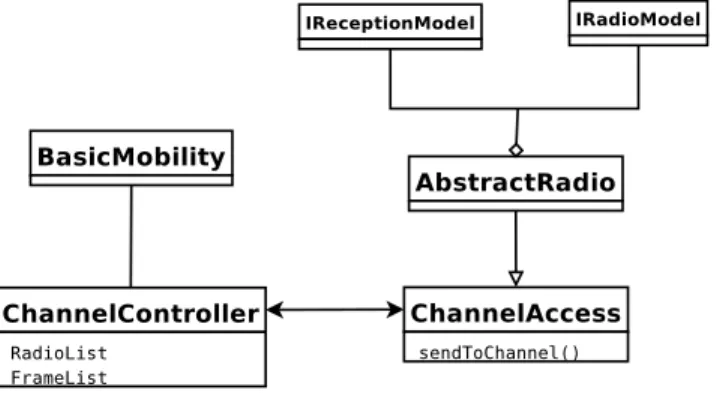
Figure 1: INET’s radio model components.

model from the computational point of view by providing quantitative data of the impact of including asymmetrical communications in the overall execution time.

The paper is organized as follows: In Section 2, the cur-rent INET implementation and features are analyzed. Sec-tion 3 depicts our proposed extension to the INET radio model for the directional antenna representation. Section 4 presents the model implementation, its main features, pa-rameters and limitations. Section 5 provides a model eval-uation by examining various antenna patterns under two well defined scenarios. Finally, Section 6 summarizes the proposed model, our main contributions and further works towards the improvement of the INET ’s radio model.

2.

STATUS OF INET MODEL

INET is an extensible network modeling framework that

consists of a set of modules, built on top of the OMNeT++ simulator. It includes sub-models for several high-level pro-tocols, such as Applications, IPv4, IPv6, SCTP, TCP, UDP, and wired and wireless physical layers. The initial design of the INET ’s radio model integrates an abstraction of the channel, called the ChannelController, with a ChannelAccess interface, which allows the AbstractRadio to interact with the radio channel. Radios are built on-top of this

Chan-nelAccess. Also, a Mobility component is provided, giving

nodes (with radio devices inside) the ability to move on the simulation playground. Fig. 1 is a class diagram of INET ’s radio model components.

The ChannelController is an abstraction of the radio chan-nels. Its main roles are: being aware of all communications (packets in the air on each channel) that are happening; registering all the simulated physical radios and their posi-tions; and determining which radios are “connected”, mean-ing which hosts are able to communicate. This latter oper-ation defines a connectivity graph, built by using the Max-imum Interference Distance to determine whether or not a radio is able to “hear” another radio, based on the Free Space propagation (Path Loss) defined by a set of identical radio parameters for all radios.

The ChannelAccess is an interface that provides the ser-vices needed to send an airframe by the channel. This in-terface is the cornerstone for implementing any radio. It is important to note that ChannelAccess interacts with the

ChannelController, both being responsible for providing the

required information to the radio in order to decide if an airframe is correctly received or transmitted.

The AbstractRadio is an extension of the ChannelAccess module. It provides a generic radio functionality, through a

RadioModel interface, which is responsible for deciding if a

packet is correctly received, based on the noise measures. It also includes a ReceptionModel interface, in charge of calcu-lating the airframe’s reception power, using a propagation loss model. There are two propagation models already im-plemented: the classical Free Space Pathloss and the

Two-ray with ground reflection.

Hosts (or nodes) contain one (or several) radio modules and one of the available Mobility modules (circular, linear, random, etc.).

The ChannelController keeps the important information needed for the AbstractRadio. Therefore, the ChannelAccess must provide means for the radio to access that information, since it is the entity that connects both sides. Moreover, as mentioned above, the ChannelController must build the con-nectivity graph (or hosts neighbors list), that indicates with which nodes communications can occur. This graph varies only in response to a mobility event, which implies that the module that triggers the graph’s update is the

BasicMobil-ity, through the ChannelController. In the current version

of INET , the communications follow a symmetrical model: For a pair of hosts h1 and h2, h2 is considered the neigh-bor of h1 if it is within its maximum interference distance, which, reciprocally, always implies that h1 is neighbor of h2 (the ChannelController uses the same maximum transmis-sion power for all radios, when calculating their maximum interference distance).

Currently1_{, there are several INET branches that}

intro-duce improvements in different ways. In particular, the branch supporting multiple radios assigns a neighbors list to each host’s radio instead of to a single list to the host. Therefore, each host has as many lists as radios. This change implies that the responsibility for building and updating the connectivity graph is transferred from the host to the radios of the host when a mobility event occurs.

3.

EXTENSIONS

TO

INET’S

RADIO

MODEL

In this section, we introduce our proposed extension to

INET ’s radio model to support directional wireless

com-munications. We start with some technical concepts, fol-lowed by the description of our proposed extension. Then, we present an extended module for the INET model, that supports directional and omni-directional communications. Notice that the problem of asymmetrical communications addressed hereafter is deeper studied in Section 4.

3.1

Concepts

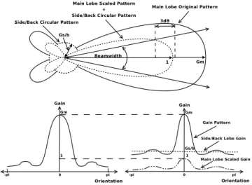
Antenna patterns are commonly used when studying propagation of radio signals in the space. The antenna

pat-tern[5] is a polar chart that describes the dependence of the

radiation power (usually in relative decibels, dB) and the di-rection of communication in 360◦_{. For omni-directional}

tennas, the theoretical pattern is a circle. For directional an-tennas, it is an irregular shape, having in general a principal or main lobe and side/back lobes. For directional patterns, the main lobe corresponds to the region where the largest amount of power is radiated, and can be characterized by its maximum gain and its Beam Width, corresponding to the

beam wideness, often defined by a 3dB-threshold[6] that de-limits it. Side/back lobes regions can also be distinguished, where smaller amounts of power are radiated (generally seen as losses) with no preferential direction. These losses are of-ten characterized by their maximum gain. In order to quan-tify the signal propagation, the Link Budget[15] equation is used. This equation corresponds to an account of the trans-mission power, antennas gains and losses. The main contri-butions are the transmission power, antennas gains and free space propagation loss.

3.2

Proposed Extension for the Radio Model

Our proposed extension to the INET ’s radio model al-lows representation of any antenna pattern, and specifically, to represent any gain function when calculating the Link

Budget for a wireless communication. Our extension

sepa-rates the Link Budget into two phases: the calculation of the antenna’s gain in a pluggable external module, and the calculation of the effective reception power on the receiv-ing end. In this model, the transmission and reception gain patterns are assumed to be identical, due to the Reciprocity theorem[11]. This helps to apply the same procedure for the gain calculation, both for transmitting and receiving an airframe. In more detail, the external pluggable module is an abstraction of an antenna pattern, that gives the gain value in the direction of two-nodes communication. Our proposed extension uses this external module to calculate the Link Budget when determining the effective transmission

power of an airframe. For two wireless hosts, the

commu-nication angle can be calculated from the transmitter’s and receiver’s coordinates, and consequently, the antenna gain in that direction can be determined. The effective

transmis-sion power is obtained by adding this gain and the nominal

antenna transmission power. A similar calculation is per-formed to determine the effective reception power, but using the received power (i.e. the difference between the effective transmission power and the path loss) instead of the nomi-nal transmission power. More formally, for omni-directionomi-nal communications, the simplified Link Budget expression is as follows:

Prx = Ptx− P L (1)

when considering the antenna gains for directional comuni-cation, the expresion becomes as:

Prx = Ptx+ Gtx− P L + Grx (2)

where Ptx is the nominal transmission power, Gtx is the

transmitter gain, Grx is the receiver gain, P L is the path

loss and Prxis the effective received power.

The advantages of separating the antenna gain from the

Link Budget is the flexibility introduced by the

externaliza-tion of the antenna gain calculaexternaliza-tion, allowing us to imple-ment any antenna pattern without changing the radio func-tionalities. Directional and omni-directional antenna pat-terns can be implemented by describing the antenna gain with mathematical curves, as well as by mapping techniques. We used a simplified Link Budget expression that only con-siders the antenna gains and propagation losses, as expressed in Equation 2, while losses due to cables, connectors, or any other type of losses are not considered.

We use the previous described extensions to implement four directional antenna patterns, based on the “pie-wedge” model described by Gharavi et al. in [7]. The radiation

pat-Figure 2: Example of antenna pattern and the scaled antenna pattern.

tern is represented by two main components: a main lobe and side/back lobes. We used different mathematical curves (folium, cardioid, circle and rose) to analytically define the main lobe’s gain function in every direction (from 0◦_{to 360}◦_);

and a circle with an unity-gain (onmi-directional communi-cation) to represent the side/back lobes. Then, while the gain of the main lobe varies according to the mathematical formula evaluated in different points, defined by the trans-mission/reception angle, the gain of the side/back lobes re-mains constant. For practical reasons, we scale the original analytical curve that defines the main lobe gain pattern, in order to obtain a curve with a maximum gain of Gm in the

main beam direction. Also, the side/back lobes are rep-resented by a circular unity-gain pattern, which multiplied by the side/back lobes gain, gives the circular pattern with radius Gs/b. Fig. 2 depicts the original and the scaled

ana-lytical curves used by the proposed directional radio, where we observe the gain function before and after the scaling. Note that the maximum gain remains the same, but now the gain function corresponds to the maximum between the main lobe scaled gain and the side/back lobes gain. This means that within the area defined by the 3dB-threshold, the main lobe gain dominates, while within the rest of the space, the gain value alternates between the main lobe scaled curve and the the side/back lobes circle.

4.

MODEL IMPLEMENTATION

In this Section, we describe the implementation of our proposed directional radio module. This implementation can be separated into two different parts: i) the modifica-tions that have to be made to current INET version when implementing asymmetrical communications; and, ii) the changes made to incorporate directional communications, including four different antenna patterns and the proposed

Link Budget calculation presented in the previous section.

4.1

Asymmetrical Communications

Our INET branch extends the multiple radios branch to support asymmetrical communications, where radios no

longer are assumed to have the same antenna pattern and transmission power. It also allows the user to select one of the implemented antenna patterns, or create a new one. This improvement forces to change the way the neighbor lists are calculated and updated, since the premise if you

hear me, I can hear you, is not always true[10] when

consid-ering asymmetrical communications.

The first step to implement asymmetrical communications on the current INET radio model, is to relieve the

Channel-Controller of the responsibility of calculating the maximum

interference distance. According to an asymmetrical radio model, radios may have different coverages (in range and in shape). Thus, this task should be assigned to the radio itself, implementing it at the AbstractRadio level. Consequently, the ChannelAccess interface would rely on the

ChannelCon-troller to build the neighbors list, but now using a method

provided by the radio to determine when a node is under its radio coverage. This method, called isInCoverageArea, relies on the ReceptionModel to determine the maximum interfer-ence distance, according to the antenna’s radiation shape, and also to the radio signal propagation model.

Regarding the connectivity graph determination, the event that triggers an update in our implementation is not only a mobility event, but a mobility event or a transmission request, since the neighbor list of any node must be updated when transmitting a packet, and so, be faithful with the ra-dio signals that each node receives. Additionally, this update is now related to all nodes (and radios) in the simulation, and not only to the node that has changed its position. These modifications have a detrimental impact on the overall ex-ecution time. Firstly, the neighbor discovery algorithm has now a complexity of O(n2_{m), n being the number of hosts,}

and m the number of radios per host; and secondly, this al-gorithm is executed more often. Preliminary results shown that the computational cost is higher enough to make the model not attractive to users when using this algorithm of “brute force” to update the neighbor lists. So, we developed an alternative algorithm that exploits the locality of nodes to calculate their neighbors lists and supports different cov-erage ranges. In Section 5.2, we analyze the computational cost of both algorithms in terms of the execution time. The next section presents the proposed algorithm for the neigh-bor list calculation.

4.2

NeighborsGraph Algorithm

In the previous section, we showed the need for an efficient algorithm to overcome the increase of the model’s execution time when using asymmetrical communications. This algo-rithm should exploit the locality of nodes, since when a sin-gle node moves, let’s say node N1, the neighbors lists that

must be updated are only those that change due to N1’s

movement, meaning the inclusion or the exclusion of N1 as

a neighbor. Updating a node that is far away from N1 is

useless, in terms of the propagation model and noise levels. This leads to our selective neighbor list update algorithm.

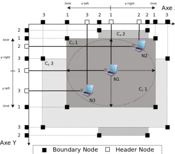
This algorithm uses a data structure, similar to a sparse matrix, but keeping the positions of nodes (in fact, radio positions) and a coverage area (Figure 3). This area, Cs, is

the square box that contains the real coverage area Cr. The

boxed coverage area Csis defined by the maximum

interfer-ence distance given a propagation model, when the received power is equal to the noise level. In the case of the Pathloss model, this distance depends on the transmitter power,

car-rier frequency and Pathloss coefficient. This distance defines Cs, which is used by the algorithm to compute the

neigh-bors list within this region. Afterwards, a refinement of this list can be made by using the isInCoverageArea method of each radio to get the real neighbors list (nodes within Cr).

It is worth to notice that the isInCoverageArea method is now applied to a reduced set of nodes, instead of all nodes in the simulation. Additionally, the neighbor list calculation returns the list of nodes to be updated as a consequence of N1’s displacement. For all those nodes, their neighbor lists

are tagged as invalid, forcing them to be updated when the node wants to transmit a packet. The algorithm determines

Figure 3: NeighborsGraph data structure the neighbor list for a node N1by exploring the sparse

ma-trix axes on each direction: x-left, y-right, x-right and y-left; finding the header nodes within the region Cs. It also

determines the updated list by finding the boundary nodes that are traversed by N1. Each node’s position (header and

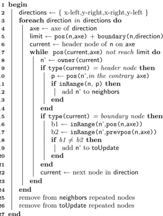
boundary nodes) is updated every time the node moves in a O(log(n)) operation, since the matrix axes are red-black trees[8]. A formal pseudo-code for the proposed algorithm is shown in Algorithm 1.

The function pos(node, axe) returns the position of the node on the given axe; boundary(node, direction) re-turns the Cs boundary limit in the given direction; and

owner(node) returns the reference to the host/radio of the node. As Figure 3 shows, each host has a header node, referencing the host position on each axe, and four bound-ary nodes, referencing the limits of the region Cs. All these

nodes have a direct reference to their host/radio module. Fi-nally, the function inRange(node, position) returns whether the given position is within the Cs region, or not. As we

al-ready mentioned, after the execution of this algorithm, the real coverage of each radio inside the node n is evaluated for each neighbor host, in order to determine the real neigh-bors list. All neighbor lists belonging to a host contained in the toU pdate list are invalidated, thus, forcing them to be updated when the host sends a packet to the channel.

The complexity of this algorithm may be higher than the brute force update algorithm on a single host, since it visits

Input: node n, empty neighbors and toUpdate lists Output: updated neighbors list and toUpdate list begin

1

directions← { x-left,y-right,x-right,y-left }

2

foreach direction in directions do

3

axe← axe of direction

4

limit← pos(n,axe) + boundary(n,direction)

5

current← header node of n on axe

6

while pos(current,axe) not reach limit do

7

n‘← owner(current)

8

if type(current) = header node then

9

p← pos(n‘,in the contrary axe)

10 if inRange(n, p) then 11 add n‘ to neighbors 12 end 13 end 14

if type(current) = boundary node then

15 b1 ← inRange(n‘,pos(n,axe)) 16 b2 ← inRange(n‘,prevpos(n,axe)) 17 if b1 6= b2 then 18 add n‘ to toUpdate 19 end 20 end 21

current← next node in direction

22

end

23

end

24

remove from neighbors repeated nodes

25

remove from toUpdate repeated nodes

26

end

27

Algorithm 1: The NeighborsGraph Algorithm.

each node at least two times (x and y directions). But, we improve the performance by doing this operation only for the nodes affected when a certain node moves, instead of updating the neighbor list of all nodes in the simulation. Performance evaluation results are given in Section 5.2.

4.3

DirectionalRadio Module

Based on the proposed extension of INET ’s radio model, we created the DirectionalRadio module, which comple-ments the current radio implementation with new function-ality. In order to make this module flexible enough to allow several antenna patterns, an AntennaPattern interface has been added. This interface contains the specific operations of a directional antenna and enables the implementation of new antenna patterns, without interfering with existing ba-sic radio operations.

As stated in Section 3, the main lobe curve is scaled to 1 (i.e. its maximum value is Gm), according to the main

lobe width as specified in the configuration file. For a given direction of communication, the gain is given by the higher value between the main lobe’s and the side/back lobes’ gain. We provide four antenna patterns, which use known math-ematical curves: CircularPattern, CardioidPattern,

Foli-umPattern and RosePattern. These antenna patterns are

customizable by changing the settings in the configuration file.

There are some parameters common to all patterns, proper to directional antennas: the beamWidth, the angular distance that indicates the main lobe width, in degrees; the

mainLobeGain, the maximum gain of the main lobe,

mea-sured in dB; the sideLobeGain, the maximum gain of the side/back lobes, in dBi; the mainLobeOrientation, which in-dicates the direction at which the main lobe is pointing, in degrees; the dBThreshold, the threshold value that defines the main lobe area, in dB; and the patternType, the selected antenna pattern shape, specified by its name. There are also some specific parameters to each case. For example, if using the CircularPattern, the radio r must be set, or the a and b parameters for the FoliumPattern.

5.

MODEL EVALUATION

We evaluated two aspects of our proposed directional ra-dio module implementation: its correctness and its compu-tational cost. The correctness of the model implementation is evaluated by comparing our simulation results with simi-lar ones found in the literature. The computational cost is estimated by measuring the execution time of the same sim-ulation model with three different scenarios: a symmetrical model scenario, an asymmetrical model scenario with full update of neighbors, and an asymmetrical model scenario with the neighbors-graph algorithm to compute and update the neighbors.

5.1

Correctness of the Proposed

Directional-Radio Module

We designed two simulations to validate and evaluate the correctness of our implementation of the DirectionalRadio module. The first one is intended to obtain and analyze the simulated antenna pattern. The second is intended to compare the performance of omni-directional and directional communications.

5.1.1

Obtaining an Antenna Pattern

This simulation has two objectives: to exhibit the an-tenna pattern, and to verify how it changes according to the transmitter-receiver distance and the path loss effect. The pattern obtained through the simulation is expected to match the settings given in the configuration file. The sim-ulated scenario consists of one directional AP with the main lobe oriented at 90◦_{, and 10 omni-directional hosts following}

a circular path with different radiuses surrounding the AP. The simulation begins with all hosts aligned at 0◦_and

sepa-rated by 10 meters each, and ends when all hosts are back to their initial position after a complete revolution around the AP. For each host, each Beacon’s Received Power is logged to assess whether the beacon was correctly received, or not. The FoliumPattern antenna was selected for this simula-tion. The radio parameters set for this simulation are shown below as an excerpt from the configuration file.

# Antenna Pattern Parameters

**.ap1.wlan.radio.transmitterPower = 40.0mW **.ap1.wlan.radio.beamWidth = 40deg **.ap1.wlan.radio.mainLobeGain = 15dB **.ap1.wlan.radio.sideLobeGain = -5dBi **.ap1.wlan.radio.mainLobeOrientation = 90deg **.ap1.wlan.radio.dBThreshold = 3dB # Folium Pattern **.ap1.wlan.radio.patternType = "FoliumPattern" **.ap1.wlan.radio.FoliumPattern.a = 1 **.ap1.wlan.radio.FoliumPattern.b = 3

Fig. 4 shows the observed antenna pattern for different dis-tances between transmitter and receiver. The angular axis corresponds to the angle between the AP and the hosts,

while the radial axis corresponds to the received power in milliwatts (mW). 10m 20m 30m 40m 50m 60m 70m 80m 90m 100m

Figure 4: Observed folium pattern at different dis-tances transmitter/receiver obtained from the sim-ulation.

We successfully verified that the antenna pattern matches with the set folium curve and its orientation. Regarding the side/back lobes, we can observe how the gain value alter-nates between the folium curve and the circle, depending on what is the higher value, as described in the implementation section. We can observe that the received power varies ac-cording to the distance between transmitter and receiver due to the path loss effect. Following one radial direction, the difference between two consecutive level curves corresponds to the path loss when the radio signal travels 10 meters.

5.1.2

Omni-directional vs. Directional

Communica-tions

The goal of the second simulation is to evaluate our

Di-rectionalRadio by comparing the network throughput when

using omni-directional and directional antennas. For this purpose, we build a mesh network simulation, with 10 nodes containing 2 bridged radio interfaces, and 2 client hosts with a single radio interface. In this scenario, the radio parame-ters for the hosts are chosen such that directional antennas are able to “hear” up to 5 antennas placed in their same di-rection of orientation, even when they are supposed to com-municate only with their immediate neighbors. We deter-mined that using a network with 10 hosts is enough to create strong interference between antennas and to clearly observe the behavior of communications. All antennas in the simu-lation have the same maximum transmission range, and the radio interfaces are configured as shown in Fig. 5, using the same channel. In this scenario, a TCP stream is transmit-ted first time from client1 to client2 through the mesh net-work, using omni-directional antennas (1st case) and then, a second time using directional antennas (2nd case); network throughput was monitored during the experiment.

Fig. 6 presents a comparison of the network throughput for the two cases described above. In the 1st case, we observe

Figure 5: Second evaluation scenario. Mesh network with multiple radio interfaces nodes.

that the network throughput is about half of the theoreti-cal one, which is consistent with previously obtained results [14]. In Fig. 7(a) we can see that the number of collisions using omni-directional nodes is constant for all radios, while for directional antennas (Fig. 7(b)) the number varies de-pending on the node’s position. This is because the coverage range for directional antennas is set to be greater, thus al-lowing two distant antennas to “hear” each other. The left radio of N 8, for instance, is able to hear from N 2 to N 7, leading to a greater number of collisions when receiving. The packet loss, however, is reduced when using directional an-tennas, as shown in Fig. 8(b), compared to the case that uses omni-directional antennas (Fig. 8(a)).

0 100000 200000 300000 400000 500000 600000 700000 0 50 100 150 200 250 3000 100000 200000 300000 400000 500000 600000 700000 Average Throughput (bps)

Simulation Time (sec)

Directional Radios

Omnidirectional Radios

Figure 6: Comparison of TCP throughput for the 1st and 2nd case for 30 repetitions of the simulation.

5.2

Computational cost Analysis

The introduction of asymmetrical communications gen-erates an increase in the execution time of the neighbors discovery procedure, since it can not be assumed reciprocity when building (or updating) the neighbor list. However, the computational cost can be partially decreased if a more re-fined algorithm is used. In order to evaluate the performance of each algorithm, we compare the simulation time for the same scenario when using: the current neighbor discovery procedure described in Section 2 for a symmetrical model (Procedure 1); the “brute force” neighbors discovery pro-cedure for the asymmetrical model described in Section 4.1 (Procedure 2); and the NeighborsGraph Algorithm described in Section 4.2 (Procedure 3).

The simulation scenario consists of 100 hosts, randomly moving at different speeds (up to 40 Km/h). There are 4 ac-cess points belonging to the same network, located in a 2×2

Left−Radio Right−Radio 0 20,000 40,000 60,000 80,000 100,000 120,000 N1 N2 N3 N4 N5 N6 N7 N8 N9 N10 Number of Collisions

(a) Omnidirectional radios

Left−Radio Right−Radio 0 20,000 40,000 60,000 80,000 100,000 120,000 N1 N2 N3 N4 N5 N6 N7 N8 N9 N10 Number of Collisions (b) Directional radios

Figure 7: Comparison for packet collisions for the 1st and 2nd case. Left−Radio Right−Radio 0 50 100 150 200 250 300 N1 N2 N3 N4 N5 N6 N7 N8 N9 N10

Number of Packet lost

(a) Omnidirectional radios

Left−Radio Right−Radio 0 50 100 150 200 250 300 N1 N2 N3 N4 N5 N6 N7 N8 N9 N10

Number of Packet lost

(b) Directional radios

Figure 8: Comparison for packet losses for the 1st and 2nd case.

grid, covering all the simulation playground and connected to a server via wired links. All radios in simulation (APs and hosts) have the same radio parameters. The hosts are expected to associate to the network performing handover

when passing from one AP’s coverage area to another’s. All along the simulation, hosts are sending ICMP traffic (ping) to the server. The simulation time was set to 500 seconds and 10 repetitions for each model were ran, logging the real execution time for each case. The hardware used to sim-ulate this scenario was a Dell Precision T3400 (Intel(R) Core(TM)2 Duo CPU E6550 @ 2.33GHz, 2Gb RAM run-ning Fedora 11).

Symetrical Model

Asymmetrical Model Brute Force Update

Asymmetrical Model NeighborGraph Update

Execution Time (seconds)

0 1000 2 000 3000 4000 5000 6000

Procedure 1 Procedure 2 Procedure 3

1156.85 sec [1122 .. 1191] 5479.6 sec [5365 .. 5593] 1500 sec [1455 .. 1545]

Figure 9: Execution time for Symmetrical and Asymmetrical model with different neighbors list update algorithms.

Figure 9 shows the execution time for the Procedures 1, 2 and 3, respectively. We can observe that using Procedure 2 increases ≈ 500% the computation time compared with Procedure 1, while the increase is close to a 50% when using Procedure 3. A comparison of means[13] among the pro-cedures shows that, while the difference between Procedure 1 and Procedure 2 is always large, the difference between Procedure 1 and Procedure 3 always remains about 50%.

We realize that Procedure 1 takes advantage from the as-sumption of symmetry of communications when determining the nodes to be updated, having a very good performance in execution time. Contrarily, when asymmetrical commu-nications are used, the neighbors list must be updated much more often to honor the SNR and noise calculation and this is done for all nodes when a host moves or transmits an airframe. Thus, the execution time is increased dramat-ically. Nevertheless, our proposed algorithm to calculate the neighbors overcomes this impact, reducing the increase in execution time reasonably when using an asymmetrical communications radio model.

Extending these results to larger simulations, we estimate that the execution time of our proposed algorithm will be always higher than the execution time when symmetrical communications are used. However, further experimenta-tion has shown that this difference is always around 50%. As we stated in Section 4.2, the execution time of the neigh-bors graph algorithm is expected to be higher since each neighbor node is visited at least twice (axe-x and axe-y).

But, a possible alternative to overcome this overhead could be to perform this exploration in a parallel way (exploiting the multi-core architectures). Whether or not the execution time of the neighbors graph algorithm could be improved, it will never be better than the algorithm for symmetrical communications, since the assumption of symmetry gives the best case when all radio coverages are equal. On the contrary, our algorithm ensures a good approximation of the optimal case when calculating the neighbors lists for a node, not only when radios coverages are equal, but also in cases where radios coverages are different in shape and size.

6.

CONCLUSIONS

In this work, we presented an extension of the

OM-NeT++ ’s INET Framework for directional and

asymmetri-cal wireless communications. This new extension is based on the existing INET multi-radio branch and introduces the following contributions: an asymmetrical Radio Model to support directional antenna patterns; a NeighborsGraph Algorithm to speed up the neighbor nodes update computa-tion; and an implementation of a Directional Radio module with four antenna patterns. The included antenna patterns use mathematical curves to represent the gain pattern in a pie-wedge directional radiation model.

Although the proposed model still has several simplifica-tions, we demonstrated through simulations that the results obtained agree with the results found in the literature when using directional radios in mesh networks.

Furthermore, despite the increase in execution time could be potentially high when using asymmetrical communica-tions, we showed it is possible to reasonably reduce it by using our NeighborsGraph algorithm.

In this work, we also identified open issues, such as the accuracy of antenna gain in the plane, or the use of multi-core architectures to speed-up the construction/update of the neighbors list. First, antenna gain can be described through a set of points by using mapping techniques; and second, the use of threading to explore on each axe direction when using the NeighborsGraph algorithm.

Finally, we consider that our contributions are a first at-tempt to provide an asymmetrical communications support within the OMNeT++/INET Framework.

7.

ACKNOWLEDGMENTS

The authors would like to thank everyone who helped us to write this paper. This work was partly funded by the IST-FET AEOLUS project and CONICYT Chile.

8.

REFERENCES

[1] The network simulator - ns-2. In

http://www.isi.edu/nsnam/ns.

[2] Qualnet network simulator. In

http://www.qualnet.com.

[3] Glomosim. In

http://pcl.cs.ucla.edu/projects/glomosim, 1998.

[4] Opnet modeler 7.0 gives network designers boost to optimize performance of wireless infrastructures. 2000. [5] C. A. Balanis. Antenna Theory: Analysis and Design.

Wiley-Interscience, 2005.

[6] J. J. Carr. Practical antenna handbook PRACTICAL

ANTENNA HANDBOOK. TAB Mastering Electronics

Series, Tab Electronics. McGraw-Hill Professional, 4, illustrated, annotated edition, 2001.

[7] H. Gharavi and B. Hu. Directional antenna for multipath ad hoc routing. In Consumer

Communications and Networking Conference, 2009. CCNC 2009. 6th IEEE, pages 1–5, Jan. 2009.

[8] L. J. Guibas and R. Sedgewick. A dichromatic framework for balanced trees. In SFCS ’78:

Proceedings of the 19th Annual Symposium on Foundations of Computer Science, pages 8–21,

Washington, DC, USA, 1978. IEEE Computer Society. [9] K. Hardwick, D. Goeckel, D. Towsley, K. Leung, and

Z. Ding. Antenna beam pattern model for cooperative ad-hoc networks. In ACITA, 2008, pages 209–216, 2008.

[10] D. Kotz, C. Newport, R. S. Gray, J. Liu, Y. Yuan, and C. Elliott. Experimental evaluation of wireless

simulation assumptions. In MSWiM ’04: Proceedings

of the 7th ACM international symposium on Modeling, analysis and simulation of wireless and mobile

systems, pages 78–82, New York, NY, USA, 2004.

ACM.

[11] J. D. Kraus. Antennas. McGraw-Hill Education, May 1988.

[12] K. Kucuk, A. Kavak, and H. Yigit. A smart antenna module using omnet++ for wireless sensor network simulation. In Wireless Communication Systems,

2007. ISWCS 2007. 4th International Symposium on,

pages 747–751, 2007.

[13] D. C. Montgomery and G. C. Runger. Applied

Statistics and Probability for Engineers, 4th Edition.

John Wiley & Sons, May 2006.

[14] S. Muthaiah, A. Iyer, A. Karnik, and C. Rosenberg. Design of high throughput scheduled mesh networks: A case for directional antennas. In Global

Telecommunications Conference, 2007. GLOBECOM ’07. IEEE, pages 5080–5085, Nov. 2007.

[15] T. S. Rappaport. Wireless Communications:

Principles and Practice (2nd Edition). Prentice Hall