Radiative forcing of the direct aerosol effect from AeroCom Phase II simulations

(1)

HAL Id: hal-02870344

https://hal.archives-ouvertes.fr/hal-02870344

Submitted on 30 Jun 2020

HAL is a multi-disciplinary open access

archive for the deposit and dissemination of

sci-entific research documents, whether they are

pub-lished or not. The documents may come from

teaching and research institutions in France or

abroad, or from public or private research centers.

L’archive ouverte pluridisciplinaire HAL, est

destinée au dépôt et à la diffusion de documents

scientifiques de niveau recherche, publiés ou non,

émanant des établissements d’enseignement et de

recherche français ou étrangers, des laboratoires

publics ou privés.

AeroCom Phase II simulations

G. Myhre, B. Samset, M Schulz, Yves Balkanski, S. Bauer, T. Berntsen, H.

Bian, N. Bellouin, M. Chin, T. Diehl, et al.

To cite this version:

G. Myhre, B. Samset, M Schulz, Yves Balkanski, S. Bauer, et al.. Radiative forcing of the direct

aerosol effect from AeroCom Phase II simulations. Atmospheric Chemistry and Physics, European

Geosciences Union, 2013, 13 (4), pp.1853-1877. �10.5194/acp-13-1853-2013�. �hal-02870344�

(2)

Atmos. Chem. Phys., 13, 1853–1877, 2013 www.atmos-chem-phys.net/13/1853/2013/ doi:10.5194/acp-13-1853-2013

EGU Journal Logos (RGB)

Advances in

Geosciences

Open Access

Natural Hazards

and Earth System

Sciences

Open Access

Annales

Geophysicae

Open Access

Nonlinear Processes

in Geophysics

Open Access

Atmospheric

Chemistry

and Physics

Open Access

Atmospheric

Chemistry

and Physics

Open Access Discussions

Atmospheric

Measurement

Techniques

Open Access

Atmospheric

Measurement

Techniques

Biogeosciences

Open Access Open Access

Biogeosciences

Discussions

Climate

of the Past

Climate

of the Past

Discussions

Earth System

Dynamics

Earth System

Dynamics

Discussions

Geoscientific

Instrumentation

Methods and

Data Systems

Open Access

_{Geoscientific}

Instrumentation

Methods and

Data Systems

Geoscientific

Model Development

Geoscientific

Model Development

Discussions

Hydrology and

Earth System

Sciences

Open Access

Hydrology and

Earth System

Sciences

Ocean Science

Discussions

Solid Earth

Discussions

The Cryosphere

Discussions

Natural Hazards

and Earth System

Sciences

Open Access

Discussions

Radiative forcing of the direct aerosol effect from AeroCom Phase II

simulations

G. Myhre1, B. H. Samset1, M. Schulz2, Y. Balkanski3, S. Bauer4, T. K. Berntsen1, H. Bian5, N. Bellouin6,*, M. Chin7, T. Diehl7,8, R. C. Easter9, J. Feichter10, S. J. Ghan9, D. Hauglustaine3, T. Iversen2,11, S. Kinne10, A. Kirkev˚ag2, J.-F. Lamarque12_{, G. Lin}13_{, X. Liu}8_{, M. T. Lund}1_{, G. Luo}14_{, X. Ma}14_{, T. van Noije}15_{, J. E. Penner}13_{, P. J. Rasch}9_, A. Ruiz15,16, Ø. Seland2, R. B. Skeie1, P. Stier17, T. Takemura18, K. Tsigaridis4, P. Wang15, Z. Wang19, L. Xu13,20, H. Yu5, F. Yu14, J.-H. Yoon9, K. Zhang10,9, H. Zhang21, and C. Zhou13

1_{Center for International Climate and Environmental Research – Oslo (CICERO), Oslo, Norway} 2_{Norwegian Meteorological Institute, Oslo, Norway}

3_{Laboratoire des Sciences du Climat et de l’Environnement, CEA-CNRS-UVSQ, Gif-sur-Yvette, France} 4_{NASA Goddard Institute for Space Studies and Columbia Earth Institute, New York, NY, USA}

5_{Earth System Science Interdisciplinary Center, University of Maryland, College Park, MD, USA} 6_{Met Office Hadley Centre, Exeter, UK}

7_{NASA Goddard Space Flight Center, Greenbelt, MD, USA} 8_{Universities Space Research Association, Columbia, MD, USA} 9_{Pacific Northwest National Laboratory, Richland, WA, USA} 10_{Max Planck Institute for Meteorology, Hamburg, Germany} 11_{Department of Geosciences, University of Oslo, Oslo, Norway}

12_{NCAR Earth System Laboratory, National Center for Atmospheric Research, Boulder, CO, USA}

13_{Department of Atmospheric, Oceanic, and Space Sciences, University of Michigan, Ann Arbor, Michigan, USA} 14_{Atmospheric Sciences Research Center, State University of New York at Albany, New York, USA}

15_{Royal Netherlands Meteorological Institute, De Bilt, The Netherlands} 16_{LIFTEC, CSIC-Universidad de Zaragoza, Zaragoza, Spain}

17_{Department of Physics, University of Oxford, Oxford, UK}

18_{Research Institute for Applied Mechanics, Kyushu University, Fukuoka, Japan} 19_{Chinese Academy of Meteorological Sciences, Beijing 100081, China}

20_{Scripps Institution of Oceanography, University of California, San Diego, La Jolla, California, USA}

21_{Laboratory for Climate Studies, National Climate Center, China Meteorological Administration, Beijing 100081, China} *_{now at: Department of Meteorology, University of Reading, Reading, UK}

Correspondence to: G. Myhre (gunnar.myhre@cicero.uio.no)

Received: 31 July 2012 – Published in Atmos. Chem. Phys. Discuss.: 30 August 2012 Revised: 9 January 2013 – Accepted: 1 February 2013 – Published: 19 February 2013

Abstract. We report on the AeroCom Phase II direct aerosol

effect (DAE) experiment where 16 detailed global aerosol models have been used to simulate the changes in the aerosol distribution over the industrial era. All 16 models have esti-mated the radiative forcing (RF) of the anthropogenic DAE, and have taken into account anthropogenic sulphate, black carbon (BC) and organic aerosols (OA) from fossil fuel, biofuel, and biomass burning emissions. In addition several

models have simulated the DAE of anthropogenic nitrate and anthropogenic influenced secondary organic aerosols (SOA). The model simulated all-sky RF of the DAE from total anthropogenic aerosols has a range from −0.58 to

−0.02 Wm−2, with a mean of −0.27 Wm−2for the 16 els. Several models did not include nitrate or SOA and mod-ifying the estimate by accounting for this with informa-tion from the other AeroCom models reduces the range and

(3)

slightly strengthens the mean. Modifying the model esti-mates for missing aerosol components and for the time pe-riod 1750 to 2010 results in a mean RF for the DAE of

−0.35 Wm−2. Compared to AeroCom Phase I (Schulz et al., 2006) we find very similar spreads in both total DAE and aerosol component RF. However, the RF of the total DAE is stronger negative and RF from BC from fossil fuel and bio-fuel emissions are stronger positive in the present study than in the previous AeroCom study. We find a tendency for mod-els having a strong (positive) BC RF to also have strong (neg-ative) sulphate or OA RF. This relationship leads to smaller uncertainty in the total RF of the DAE compared to the RF of the sum of the individual aerosol components. The spread in results for the individual aerosol components is substantial, and can be divided into diversities in burden, mass extinction coefficient (MEC), and normalized RF with respect to AOD. We find that these three factors give similar contributions to the spread in results.

1 Introduction

Global estimates of the direct aerosol effect (DAE) have proved tremendously over the last two decades, due to im-provements in processes taken into account and handling of complexities in the aerosol schemes (Bauer et al., 2010; Chin et al., 2009; Seland et al., 2008; Stier et al., 2005; Take-mura et al., 2002). The first study of radiative forcing (RF) of the DAE with a global aerosol model included only sulphate aerosols (Charlson et al., 1991). Now multi-model studies with multi aerosol components and including some complex aerosol microphysical schemes have been performed (Schulz et al., 2006).

In the estimate of the RF from the direct aerosol effect from AeroCom Phase I models (Schulz et al., 2006) an-thropogenic sulphate, black carbon and organic carbon were considered. In the interim increased attention has been given to the direct aerosol effect of anthropogenic nitrate and sec-ondary organic aerosols (SOA). The formation of ammonium nitrate is complex and is dependent on sufficient ammonia and thus competition with sulphate is important (Adams et al., 2001; Metzger et al., 2002). With the expected reduc-tion in SO2emission in the future, nitrate may become more

important as a climate forcer (Bauer et al., 2007; Bellouin et al., 2011). Over the last few years increasing considera-tion has also been paid to secondary organic aerosols (SOA), with advanced understanding of their anthropogenic influ-ence (Hoyle et al., 2011; Robinson et al., 2007). Anthro-pogenic influence on SOA is now included with varying de-grees of complexity in some global aerosol models (Hoyle et al., 2009; Liao and Seinfeld, 2005; Spracklen et al., 2011; Tsigaridis et al., 2006).

The mean RF of the total direct aerosol effect in Schulz et al. (2006) from 9 global aerosol models was −0.22 Wm−2.

This is much weaker than several observational based esti-mates (Bellouin et al., 2005, 2008; Chung et al., 2005; Quaas et al., 2008). Observational based estimates have been made possible through the advancement of remote sensing from ground and space (Holben et al., 1998; Remer et al., 2008). Myhre (2009) showed that estimates of the direct aerosol ef-fect must rely on global aerosol model estimates, but con-sistency between models and observational based methods could be reached by accounting for anthropogenic changes in the aerosol optical properties in the latter method.

Various factors lie behind the large range in the global estimates of the DAE, which in AeroCom Phase I was from −0.41 to +0.04 Wm−2 (Schulz et al., 2006). Schulz et al. (2006) showed that the variations in RF could be sepa-rated into diversities in aerosol residence time, aerosol mass extinction coefficients, and normalized forcing (RF divided by aerosol optical depth). Normalized forcing was found to be the single largest contributor to the variability. Differences in the aerosol vertical profile, known to be significant be-tween the models, is among the factors that contribute to dif-ferences in the normalized RF (Heald et al., 2011; Schwarz et al., 2010; Textor et al., 2006; Zarzycki and Bond, 2010).

In this paper RF of the DAE from 16 recent state-of-the-art global aerosol models in the AeroCom Phase II are pre-sented. Two of the 16 global aerosol models are from Asia, six from Europe and eight from North America. Additional models compared to Schulz et al. (2006) are included in Phase II, and the models have been further developed over the 7–8 yr since AeroCom Phase I. Results for anthropogenic nitrate and SOA are included in the present study. Evaluation of the global aerosol models is an ongoing activity within AeroCom, with comparisons of various measurements being performed (Huneeus et al., 2011; Koch et al., 2009; Koffi et al., 2012). Activities to understand the model differences are also an important part of AeroCom (Randles et al., 2012; Samset et al., 2012; Stier et al., 2012; Textor et al., 2007).

2 Methods

The RF of the total anthropogenic DAE is calculated as the difference between the reflected solar radiation at TOA for simulations with present (2000, or 2006 for a few models) and pre-industrial (1850) emissions of aerosols and their precursors, denoted respectively as CTRL and PRE simu-lations, but the same cloud and surface conditions. The RF has been simulated by 16 global aerosol models with vari-ous complexities with regard to number of aerosol species included, aerosol microphysical treatment and their aerosol optical properties. The host model is also of great impor-tance since aerosol transport and removal is dependent on the transport scheme and distribution of precipitation, respec-tively. In the radiative transfer calculations cloud distribution and properties and surface albedo, among other factors, are important.

(4)

G. Myhre et al.: Radiative forcing of the direct aerosol effect 1855 Table 1. Model description, general information. If meteorology was nudged or driven by reanalysis fields, the year 2006 meteorology was used.

Model Type Resolution Levels Meteorology Responsible

BCC GCM 2.8°×2.8° 26 NCEP/NCAR reanalysis Hua Zhang

Zhili Wang CAM4-Oslo GCM 2.5°×1.8° 26 Produced by CAM4 atmospheric physics with

CAM4-Oslo cloud tuning and boundary data from the data ocean and sea-ice models of CCSM4.

Alf Kirkev˚ag Trond Iversen Øyvind Seland

CAM5.1 GCM 2.5°×1.8° 30 CAM5.1 X. Liu

R. C. Easter Steve Ghan P. J. Rasch J.-H. Yoon

GEOS-Chem CTM 5.0°×4.0° 47 GEOS-5, reanalysis, nudged Fangqun Yu

Gan Luo Xiaoyan Ma

GISS-MATRIX GCM 2.5°×2.0° 40 Nudged to NCEP winds Susanne Bauer

Kostas Tsigaridis

GISS-modelE GCM 2.5°×2.0° 40 Nudged to NCEP winds Kostas Tsigaridis

Susanne Bauer

GMI CTM 2.5°×2.0° 72 GEOS-5 MERRA reanalysis for 2006, nudged Huisheng Bian

Hongbin Yu GOCART CTM 2.5°×2.0° 30 GEOS-4 DAS (Goddard Earth Observing System version

4 Data Assimilation System), reanalysis for year 2006

Thomas Diehl Mian Chin IMPACT CTM 5.0°×4.0° 46 DAO assimilation fields for 1997, reanalysis. Guangxing Lin

Joyce Penner Li Xu Cheng Zhou INCA GCM 3.8°×1.9° 19 ECMWF reanalysis from the Integrated Forecast System

(IFS) model for year 2006.

Yves Balkanski Michael Schulz Didier Hauglus-taine

HadGEM2 GCM 1.8°×1.2° 38 ERA Interim data for 2006, nudged Nicolas Bellouin

ECHAM5-HAM GCM 1.8°×1.8° 31 Model nudged with ECMWF analysis for the year 2006 Kai Zhang Philip Stier Johann Feichter

NCAR-CAM3.5 GCM 2.5°×1.9° 26 GCM-generated Jean-Francois

Lamarque OsloCTM2 CTM 2.8°×2.8° 60 ECMWF reanalysis from the Integrated Forecast System

(IFS) model for year 2006

Gunnar Myhre Ragnhild B. Skeie Terje Berntsen SPRINTARS GCM 1.1°×1.1° 56 NCEP/NCAR reanalysis (temperature and horizontal

wind),nudged.

Toshihiko Take-mura

TM5 CTM 3.0°×2.0° 34 ECMWF ERA-Interim reanalysis for year 2006 Twan van Noije Ping Wang Ana Ruiz

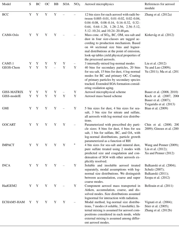
Tables 1 and 2 show a list of the models included in the AeroCom Phase II DAE experiment, together with the res-olutions used, aerosols components treated and comments on their microphysics scheme. Meteorological data for year 2006 have been used for all the models, except for IMPACT with meteorological data for 1997 and for CAM4-Oslo, NCAR-CAM3.5, and CAM5.1 where nudging possibilities were not available. A protocol describing the data submitted from the global aerosol models are available from the

Ae-roCom web site (http://aerocom.met.no/aerocomhome.html). Most of the simulations for this DAE experiment are per-formed with identical cloud cover and cloud optical proper-ties in PRE and CTRL, i.e. no indirect aerosol effects are included, but one (CAM5.1) estimated the DAE from the CTRL-PRE difference (1) in the direct radiative forcing by all aerosols in each simulation (Ghan et al., 2012): 1 (S-Sclean), where S is the net downward solar at TOA calculated

(5)

Table 2. Model description, aerosol information.

Model S BC OC BB SOA NO₃ Aerosol microphysics References for aerosol

module

BCC Y Y Y Y – – 12 bin sizes for each aerosol with radii

be-tween 0.005–0.01, 0.01–0.02, 0.02–0.04, 0.04–0.08, 0.08–0.16, 0.16–0.32, 0.32– 0.64, 0.64–1.28, 1.28–2.56, 2.56–5.12, 5.12–10.24, and 10.24–20.48 µm.

Zhang et al. (2012a)

CAM4-Oslo Y Y Y Y – – Mass conc. of SO4, BC, OM, sea-salt and dust in four size-classes are tagged ac-cording to production mechanism. Based on 44 sectional size bins and lognor-mal distributions at the point of emission, look-up tables yield physical properties of the processed aerosols.

Kirkev˚ag et al. (2012)

CAM5.1 Y Y Y Y Y – 3 internally-mixed log-normal modes Liu et al. (2012)

GEOS-Chem Y Y Y – Y Y 40 bins for secondary particles, 20 bins for sea salt, 15 bins for dust, 4 log-normal modes for BC and primary OC. Coating of primary particles by secondary species tracked. Extended SOA formation consid-ering oxidation aging.

Yu and Luo (2009); Yu (2011); Ma et al. (2012)

GISS-MATRIX Y Y Y Y – Y Aerosol microphysical scheme Bauer et al. (2008, 2010)

GISS-modelE Y Y Y Y Y Y Aerosol mass based scheme Koch et al. (2007, 2006);

Bauer et al. (2007); Tsigaridis et al. (2013)

GMI Y Y Y Y – Y 5 bin sizes for dust, 4 bin sizes for

sea-salt, 3 bin size for nitrate and sulfate, all aerosols with log-normal size distribu-tions.

Bian et al. (2009)

GOCART Y Y Y Y Y – Parameterized with prescribed dry

parti-cle sizes: 8 bins for dust, 4 bins for sea salt, 1 bin for sulfate, BC, and OA, with log-normal distributions, particle growth parameterized as a function of RH

Chin et al. (2000, 2002, 2009); Ginoux et al. (2001)

IMPACT Y Y Y Y Y ∗ 4 bin sizes for sea-salt and mineral dust,

pure sulfate treated using 2 modes with predicted size and coagulation and con-densation of SO4 with other aerosols ex-plicitly resolved.

Wang and Penner (2009); Lin et al. (2012); Xu and Penner (2012)

INCA Y Y Y Y – Y Soluble and insoluble aerosol treated

separately, modal assumptions with log-normal size distributions. We distinguish between accumulation, coarse and super coarse modes.

Balkanski et al. (2004); Schulz (2007); Balkanski (2011); Szopa et al. (2012)

HadGEM2 Y Y Y Y – Y Component aerosol mass transported in

Aitken, accumulation, coarse, and dis-solved modes. Size distributions assumed lognormal for interaction with radiation.

Bellouin et al. (2011)

ECHAM5-HAM Y Y Y Y Y – Modal method, log-normal size distribu-tions, 7 modes (4 soluble, 3 insoluble). In-ternal mixing is assumed for aerosol com-positions considered in each mode, while external mixing is assumed among differ-ent aerosol modes.

Vignati et al. (2004); Stier et al. (2005); Zhang et al. (2012b)

(6)

G. Myhre et al.: Radiative forcing of the direct aerosol effect 1857 Table 2. Continued.

Model S BC OC BB SOA NO₃ Aerosol microphysics References for aerosol

module NCAR-CAM3.5 Y Y Y Y – Y Bulk-aerosol model, except 4-bins for

sea-salt and mineral dust

Lamarque et al. (2012) OsloCTM2 Y Y Y Y Y Y 8 bin sizes for sea-salt and mineral dust,

aerosol mass scheme for other aerosols with log-normal size distributions in cal-culations of optical properties

Myhre et al. (2007, 2009); Skeie et al. (2011)

SPRINTARS Y Y Y Y – – 6 bins for dust, 4 bins for sea salt, 1 bin for sulfate, BC, and OA, with log-normal size distributions and particle growth as a function of relative humidity

Takemura et al. (2005, 2009)

TM5 Y Y Y Y Y Y Modal method, log-normal size

distribu-tions, 7 modes (4 soluble, 3 insoluble). In-ternal mixing is assumed for aerosol com-positions considered in each mode, while external mixing is assumed among differ-ent aerosol modes.

Vignati et al. (2004); Aan de Brugh et al. (2011)

Note: GOCART only includes SOA from biogenic sources (terpene oxidation) ∗_{The NO}

3values for forcing from this model were simulated using the same model as the IMPACT model described here, but did not include the chemistry of formation of SOA and used the simplified NOxchemistry described in Feng and Penner (2007). The resolution was 2.5 × 2.0.

with all aerosols present, and Sclean is the solar calculated

neglecting scattering and absorption by all aerosols.

Aerosol optical properties are treated differently in the global aerosol models but in all models the optical proper-ties are derived using Mie theory; see further description in model references. All models include treatment of sulphate, black carbon, primary organic carbon, sea salt, and mineral dust. Internal mixing between BC and scattering aerosols en-hances the absorption from BC (Fuller et al., 1999; Hay-wood and Shine, 1995), and half of the 16 models include some degree of internal mixture for BC. Most of the models have used emissions of aerosols and their precursors from Lamarque et al. (2010). CAM4-Oslo and SPRINTARS have used these IPCC AR5 emissions for PRE (year 1850), but for the CTRL simulations emissions for year 2006 from the AeroCom Phase II dataset has been used (HCA0 v1 or v2 by T. Diehl, see http://aerocom.met.no/emissions.html). This dataset also includes emissions estimates of BC, SO2 and

POM from aviation. BCC used year 2000 emissions, but preindustrial emissions for 1750. GEOS-Chem uses emis-sions for 2006 which is close to AeroCom emission for 2000 and employs pre-industry emission corresponding to 1750 (Dentener et al., 2006). TM5 used 1850 emissions from Lamarque et al. (2010) and for 2006 a linear interpolation between 2005 and 2010 for the representative concentration pathway RCP4.5 (Thomson et al., 2011).

If the diagnostics for the different components were diffi-cult to establish, separate model simulations were performed to allow for an attribution to eg biomass burning (BB) or fos-sil fuel (FF) and bio fuel (BF) sources. For some of the mod-els with internally-mixed aerosols the separation of AOD

and RF by aerosol component is challenging. Several groups have solved this by additional radiation calls. Even with this method a few models have been unable to properly extract the component AOD. Where relevant, these results have been removed from the analysis. All simulations were performed such that the cloud fields were identical, e.g. by neglecting the influence of aerosols on clouds or keeping the influence constant.

Only anthropogenic aerosol effects will be treated in the present study, and reference to the DAE apply to the anthro-pogenic change in the aerosol distribution and its influence on the scattering and absorption of solar radiation. Results will be presented for sulphate, nitrate, BC from fossil fuel and biofuel, OA from fossil fuel and biofuel, BC and OA combined from biomass burning, and SOA.

3 Results

All results are for anthropogenic aerosols only, unless other-wise stated. Anthropogenic aerosols are defined as the dif-ference between the CTRL and PRE simulations described above.

3.1 Total direct aerosol effect

The underlying albedo is crucial for RF of the direct aerosol effect (Haywood and Shine, 1995). Scattering aerosols are efficient at producing a RF over dark surfaces and absorb-ing aerosols are efficient over bright surfaces. Figure 1a shows the latitudinal variation of the top of the atmosphere (TOA) albedo of the 16 models and the satellite retrieval from

(7)

Fig. 1. Zonal mean top of the atmosphere short wave (TOA) albedo (a) and effective broadband surface albedo (b) shown for all the models. CERES TOA albedo data is shown together with the models.

Fig. 2. Zonal mean DAE RF for all-sky (a) and RF for clear sky (b).

CERES (Smith et al., 2011; Wielicki et al., 1996). Note that the albedo at the TOA consists of reflection at the surface and scattering in the atmosphere from clouds, aerosols, and Rayleigh scattering, and thus the scattering may occur above the anthropogenic aerosols. The higher albedo at high lati-tudes is mainly due to high surface albedo from snow and ice, but larger cloud fraction also contributes. For most of the models the albedo compares well to the CERES data, except between 30◦_{N and 30}◦_{S where almost all}

overesti-mate the albedo. By inspection of the geographical distribu-tion (not shown) of the albedo the overestimadistribu-tion is largest in regions with low cloud fraction, indicating problems with too large cloud fractions in these regions for the models. The GOCART model has a very low albedo compared to the rest of the models and the CERES data, which is identified to be caused by the meteorological data. The agreement be-tween the simulated latitudinal variation in effective

broad-band surface albedo (computed from surface level down and up welling short wave radiation fluxes as diagnosed in the models) is in general excellent (see Fig. 1b), except at high latitudes due to differences in snow cover or albedo for snow and for the Northern Hemisphere sea ice coverage and albedo for sea ice.

Figure 2 shows the latitudinal variation in the RF of the total DAE for all sky (Fig. 2a) and clear sky (Fig. 2b) condi-tions. The negative RF is at maximum around 30◦_{N for most}

of the models, since the anthropogenic change in aerosol burden (see Fig. 3) has its maximum in this region com-bined with a relatively high solar radiation flux. GISS-Matrix and GMI have the strongest all-sky RF in the Northern Hemisphere, but for clear-sky the IMPACT model shows the strongest RF in most of the Northern Hemisphere. The RF in the Southern Hemisphere is generally weak. How clouds affect the RF of the direct aerosol effect depends on a variety

(8)

G. Myhre et al.: Radiative forcing of the direct aerosol effect 1859

Copernicus Publications

Bahnhofsallee 1e 37081 Göttingen Germany

Martin Rasmussen (Managing Director) Nadine Deisel (Head of Production/Promotion)

Contact publications@copernicus.org http://publications.copernicus.org Phone +49-551-900339-50 Fax +49-551-900339-70 Legal Body Copernicus Gesellschaft mbH Based in Göttingen Registered in HRB 131 298 County Court Göttingen Tax Office FA Göttingen USt-IdNr. DE216566440

Page 1/1

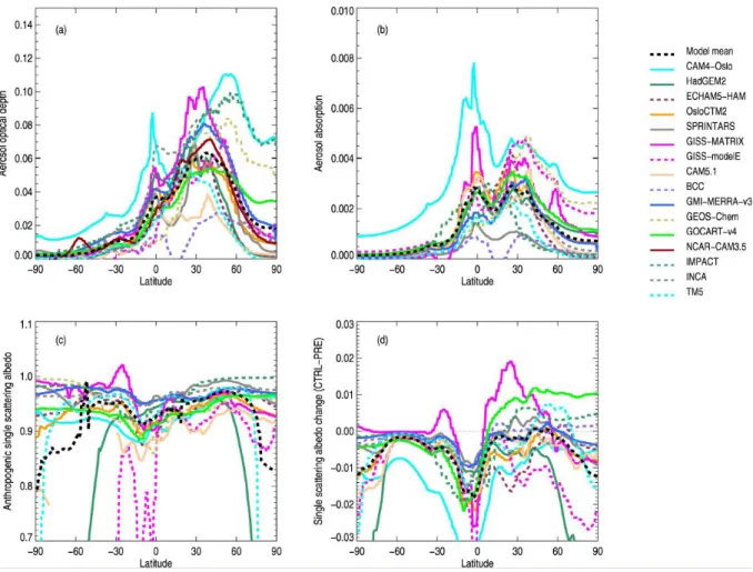
Fig. 3. Anthropogenic AOD (a), anthropogenic AAOD (b), anthropogenic single scattering albedo (c), and change in single scattering albedo from pre-industrial to present conditions (d). All values are taken at 550 nm. Between 80◦S and 30◦S the anthropogenic AOD is extremely small for some of the models and anthropogenic single scattering albedo may reach unrealistic values and in such cases values have been removed from the figure.

of factors. Among them are the degree of aerosol absorp-tion, vertical position of aerosols in relation to clouds, and the cloud distribution in general. The all-sky RF is around half in magnitude of the clear sky RF, except for the mod-els with close to zero all sky RF. All modmod-els turn over into a positive net RF at high northern latitudes. This is caused by the higher surface and cloud albedo at high latitudes, as can be seen in Fig. 1. The surface and cloud albedo is the main cause of the positive RF since it will be later shown that aerosol optical properties are not a cause for the positive RF (see Fig. 3). CAM4-Oslo has the strongest positive all-sky RF at high latitudes. This model has more anthropogenic ab-sorbing aerosols at high latitudes than the other models (see Fig. 3). This is partly due to the different CTRL emission data sets, which are for year 2006 and have more biomass burning from forest fires than the 2000 emissions. Assumed emission height of biomass burning (up to 6 km) may be an-other reason. The treatment of convective mixing of aerosols and aerosol precursors probably also leads to somewhat

over-estimated aerosol burdens in CAM4-Oslo (see Kirkev˚ag et al., 2012).

Figure 3 shows the latitudinal variation in the anthro-pogenic AOD (550 nm) used in the radiative transfer calcu-lations, anthropogenic absorbing AOD (AAOD) (550 nm), anthropogenic single scattering albedo (550 nm), and the change in single scattering albedo (550 nm) between pre-industrial (PRE) and current (CTRL). The anthropogenic AOD in Fig. 3a shows a strong hemispheric difference which is a consistent model characteristic. CAM4-Oslo has the highest and CAM5.1 and BCC the lowest anthropogenic AOD almost at all latitudes. The pattern for the anthro-pogenic AAOD (Fig. 3b) is rather similar in the models, with two peaks, one around the Equator where biomass burning emissions of BC are high, and the second around 30◦_N,

where fossil fuel and biofuel emissions of BC are high. The range in the anthropogenic single scattering albedo (de-fined as the ratio of anthropogenic AOD-AAOD and AOD) (Fig. 3c) is large, with most values lying between 0.9 and 1.0 but even lower values than 0.9 seen at high latitudes for a few

(9)

models. The lowest anthropogenic single scattering albedo is simulated near the Equator and can be seen in Fig. 3b to be caused by strong anthropogenic absorption AOD that is not associated with a similar strong maximum in the anthro-pogenic AOD in Fig. 3a. This pattern is caused by large BB emissions of BC and OA in this region. Most models sim-ulate a reduction in the single scattering albedo during the industrial era at all latitudes, except GISS-MATRIX, GO-CART, TM5 and IMPACT. The reduction in the single scat-tering albedo in the majority of the models is due to stronger growth in absorbing aerosol (BC) than scattering aerosols relative to pre-industrial distribution of absorbing and tering aerosols. GOCART has an increase in the single scat-tering albedo in the NH due to low single scatscat-tering albedo in the PRE simulation compared to most of the other models. IMPACT shows a weaker increase in single scattering albedo than GOCART, but still positive in the NH. As will be shown later this model has a much larger anthropogenic influenced SOA than the other models, which is likely the cause of the increase in single scattering albedo.

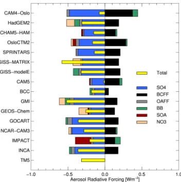
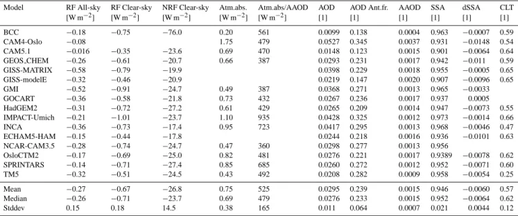
Table 3 summarizes the global and annual mean values for RF, anthropogenic AOD, anthropogenic absorption AOD (AAOD), atmospheric absorption, anthropogenic single scat-tering albedo, and cloud fraction. The anthropogenic AOD has a mean of 0.030, which is slightly higher than the Schulz et al. (2006) value of 0.029. A main reason for this small increase is likely the inclusion of additional aerosol com-ponents in this experiment. The anthropogenic AAOD of 0.0015 is lower than the value of 0.0019 for AAOD attributed to BC in Schulz et al. (2006). However, here it should be mentioned that some of the models in this experiment in-clude absorption by OA which is non-negligible at 550 nm and thus the anthropogenic AAOD is not solely due to BC. A main reason for the lower AAOD compared to Schulz et al. (2006) is likely due to the much smaller anthropogenic BB emissions of BC in a majority of the models using the Lamarque et al. (2010) data. Figure 4 shows the model simu-lated global and annual mean total RF and the RF for the six aerosol components. The simulated mean RF for the DAE is −0.27 Wm−2 which is stronger negative than the mean of −0.22 Wm−2 found in Schulz et al. (2006). A stronger negative RF of the DAE in this experiment than in Schulz et al. (2006) is in accordance with the stronger AOD and weaker AAOD as noted above. It can also be noted that the models in this experiment have lower global and annual mean cloud cover (mean of 57 % for the 13 models reporting cloud cover) than in the models in Schulz et al. (2006) (mean of 63 %). As shown in many previous studies of the DAE the total RF consists of aerosol components causing negative RF and positive RF. Figure 4 shows clearly that this balance varies substantially between the models. Further, it shows that some models have weak RF for the aerosol compo-nents (CAM5 and BCC) whereas other models have stronger aerosol component RF (CAM4-Oslo, OsloCTM2 and GMI).

Fig. 4. Radiative forcing from the six components, overlain with the (unmodified) model total forcing (yellow bars).

Not all models have all six aerosol components included. Figure 5 shows the total RF where modifications for miss-ing aerosol components have been taken into account. We calculate the mean of each aerosol component from all mod-els that treat it, then add that mean to the total RF for each component that an individual model doesn’t treat. Since the missing aerosol components in the models are predominantly scattering aerosols (nitrate, SOA, and in some few cases BB aerosols), the modification leads to stronger negative RF for all models with modification. The mean RF of the DAE changes from −0.27 Wm−2to −0.32 Wm−2with the aerosol component modification.

Table 3 also shows the normalized clear sky RF (NRF, clear sky RF divided by AOD), which ranges from

−17 Wm−2to −76 Wm−2with a mean of −27 Wm−2. The NRF depends on a variety of factors such as spatial dis-tribution, optical properties, and the vertical profile. The weakening of the DAE RF due to clouds (Schulz et al., 2006) depends on vertical positioning of the aerosols and the clouds (Chand et al., 2009; Liao and Seinfeld, 1998; Sam-set and Myhre, 2011) as well as the degree of absorption of the aerosols (single scattering albedo) (Haywood and Shine, 1995).

Atmospheric absorption by the aerosols is calculated as the difference between the RF at TOA and radiative ef-fect of aerosols at the surface. Absorbing aerosols such as BC are the main cause for the atmospheric absorption by the aerosols, but scattering aerosols enhance the absorption by gases in the atmosphere and make a small contribution (Randles et al., 2012; Stier et al., 2012). Figure 6 shows

(10)

G. Myhre et al.: Radiative forcing of the direct aerosol effect 1861 Table 3. Global mean anthropogenic value for all-sky and clear sky RF, normalized RF (NRF) with respect to AOD for clear sky, at-mospheric absorption, atat-mospheric absorption divided by AAOD, AOD, anthropogenic fraction of AOD, AAOD, single scattering albedo (SSA), combined natural and anthropogenic change in SSA from PRE simulation to CTRL simulation, and present day cloud fraction (CLT). For NCAR-CAM3 the sum of component forcings is used.

Model RF All-sky RF Clear-sky NRF Clear-sky Atm.abs. Atm.abs/AAOD AOD AOD Ant.fr. AAOD SSA dSSA CLT [W m−2] [W m−2] [W m−2] [W m−2] [W m−2] [1] [1] [1] [1] [1] [1] BCC −0.18 −0.75 −76.0 0.20 561 0.0099 0.138 0.0004 0.963 −0.0007 0.59 CAM4-Oslo −0.08 1.75 479 0.0527 0.345 0.0037 0.931 −0.0148 0.54 CAM5.1 −0.016 −0.35 −23.6 0.69 470 0.0148 0.123 0.0015 0.901 −0.0064 0.64 GEOS CHEM −0.26 −0.61 −20.7 0.66 387 0.0293 0.231 0.0017 0.942 −0.011 0.59 GISS-MATRIX −0.58 −0.79 −19.9 0.0398 0.229 0.0018 0.955 −0.0005 0.65 GISS-modelE −0.32 −0.46 −20.9 0.0219 0.147 0.0020 0.907 −0.0096 0.65 GMI −0.52 −0.91 −24.7 0.49 387 0.0368 0.271 0.0013 0.965 −0.0033 GOCART −0.36 −0.58 −21.8 0.73 432 0.0267 0.236 0.0017 0.937 0.0005 HadGEM2 −0.31 −0.72 −27.2 0.61 429 0.0265 0.209 0.0014 0.947 −0.0073 0.55 IMPACT-Umich −0.21 −1.01 −23.7 1.10 935 0.0428 0.325 0.0012 0.973 −0.0014 0.66 INCA −0.36 −0.73 −17.4 0.95 723 0.0417 0.295 0.0013 0.968 −0.0046 0.47 ECHAM5-HAM −0.15 −0.44 −17.8 0.0244 0.218 0.0016 0.936 −0.0101 0.63 NCAR-CAM3.5 −0.28 −0.74 −24.7 0.47 360 0.0298 0.277 0.0013 0.956 OsloCTM2 −0.17 −0.69 −25.0 0.82 481 0.0276 0.221 0.0017 0.9389 −0.0078 0.62 SPRINTARS −0.14 −0.71 −27.4 0.85 685 0.0260 0.272 0.0012 0.952 −0.0071 0.60 TM5 −0.32 −0.51 −24.5 0.43 492 0.0208 0.282 0.0009 0.958 −0.0054 0.25 Mean −0.27 −0.67 −26.8 0.75 525 0.0295 0.239 0.0015 0.946 −0.0060 0.57 Median −0.26 −0.71 −23.7 0.69 479 0.0276 0.233 0.0015 0.952 −0.0064 0.62 Stddev 0.15 0.18 14.5 0.38 165 0.011 0.064 0.0007 0.021 0.0044 0.12

Table 4. Anthropogenic load, mass extinction coefficient (MEC), AOD, RF, normalized RF with respect to burden (NRFB), normalized RF with respect to AOD (NRFA) for sulphate.

Model Load MEC AOD RF NRFB NRFA

[mg m−2] [m2g−1] [1] [W m−2] [W g−1] [W m−2] BCC 1.29 5.4 0.0069 −0.14 −108 −20.0 CAM4−Oslo 2.78 12.3 0.0342 −0.48 −173 −14.0 CAM5.1 1.69 5.6 0.0095 −0.18 −104 −18.4 GEOS CHEM 1.57 7.3 0.0114 −0.19 −123 −16.8 GISS-MATRIX 1.54 −0.30 −196 GISS-modelE 1.03 38.6 0.0398 −0.32 −307 −8.0 GMI 2.14 12.0 0.0256 −0.42 −195 −16.3 GOCART 1.87 12.2 0.0228 −0.44 −238 −19.5 HadGEM2 1.59 8.9 0.0142 −0.31 −193 −21.7 IMPACT-Umich 1.42 10.3 0.0146 −0.16 −113 −11.0 INCA 2.26 12.5 0.0283 −0.41 −180 −14.4 MPIHAM 2.25 9.1 0.0204 −0.28 −125 −13.8 NCAR-CAM3.5 1.27 23.2 0.0295 −0.45 −354 −15.1 OsloCTM2 1.82 10.1 0.0183 −0.35 −192 −19.0 SPRINTARS 2.13 10.3 0.0220 −0.37 −172 −16.6 Mean 1.78 12.7 0.0213 −0.32 −185 −16.0 Median 1.69 10.3 0.0212 −0.32 −180 −16.5 Stddev 0.47 8.6 0.0096 0.11 71 3.7

the atmospheric absorption by anthropogenic aerosols as a function of absorbing AOD. The mean atmospheric absorp-tion (see Table 3) is 0.75 Wm−2, which is weaker than the 0.82 Wm−2 _{reported in Schulz et al. (2006). The}

normal-ized values (atmospheric absorption divided by absorbing AOD) are shown on the figure. Normalized values range from 360 Wm−2to 935 Wm−2with a mean of 525 Wm−2and the

median 10 % lower. Some of the models with lowest anthro-pogenic atmospheric absorption have the largest deviation from the mean of the normalized values. The correlation be-tween anthropogenic absorption AOD and atmospheric ab-sorption is 0.73 for the 12 models available for this part of the study. IMPACT has high atmospheric absorption mainly, as discussed above, due to a large fraction of SOA that absorbs

(11)

Fig. 5. Model total RFs. Black bars show the bare modelled forc-ing, the colored bars show the forcing modified for untreated com-ponents (see text for details). The yellow bar shows the AeroCom mean of the total RF of DAE. Solid lines inside the boxes show the model mean, dashed lines show the median. The boxes indicate one standard deviation, while the whiskers indicate the max and min of the distribution. The yellow shaded bar shows the AeroCom mean when aerosol component adjustment is made for missing aerosol components.

Fig. 6. Correlation between anthropogenic absorption AOD and atmospheric absorption. Numbers show ratio AtmAbs/AAOD, the lines indicate the mean and one standard deviation of this ratio.

R2=0.73

Fig. 7. Component and total RF. Total RF has been modified for missing components in individual models. Solid lines inside the boxes show the model mean, dashed lines show the median. The boxes indicate one standard deviation, while the whiskers indicate the max and min of the distribution.

at short wavelengths, while the absorption is much weaker at 550 nm which is the reported wavelength for absorption AOD. This leads to the strongest normalized atmospheric ab-sorption of 935 Wm−2for IMPACT. The mean of the anthro-pogenic fraction of AOD (Table 3) is 24 %, slightly smaller than in Schulz et al. (2006), where a different preindustrial year (here 1850 instead of 1750) is one contributor to this reduction. Half of the models are close to the mean anthro-pogenic fraction, whereas two of the models have quite low anthropogenic fractions of 12–14 % and one has 35 %.

Figure 7 summarizes the component and aerosol com-ponent modified total RFs and their intermodel variability. Model means are shown as solid lines in the middle of the boxes, median values as dashed lines. The boxes indicate one standard deviation, and the bars show the maximum and min-imum single values.

In the following sections we discuss the individual aerosol components in detail, highlighting model results that deviate significantly from the mean.

3.2 RF of sulphate

The RF of the direct aerosol effect of sulphate is shown in Fig. 4 for all models. In addition Figure 7 shows the mean, median, standard deviation and the range for sulphate aerosols and for other aerosol components. Table 4 summa-rizes the aerosol burden, mass extinction coefficient (MEC) (550 nm), AOD (550 nm), RF, and NRF with respect to both burden and AOD. The mean RF of sulphate from the Ae-roCom Phase II models of −0.32 Wm−2is weaker than the mean of AeroCom Phase I models of −0.35 Wm−2in Schulz et al. (2006). The range in RF is very similar in the two Aero-Com DAE experiments. The global mean MEC is calculated as the ratio of global mean AOD to global mean burden. The

(12)

Fig. 8. Zonal mean SO4RF (a), burden (b), AOD at 550 nm (c), normalized RF with respect to AOD (NRF(A)) (d).

Table 5. Same as Table 4 for BC from FF and BF emissions.

[mg m−2] [m2g−1] [1] [W m−2] [W g−1] [W m−2] BCC 0.08 4.2 0.0003 0.05 650 155.1 CAM4-Oslo 0.21 8.2 0.0017 0.37 1763 216.0 CAM5.1 0.07 18.6 0.0014 0.20 2661 143.3 GEOS CHEM 0.12 8.2 0.0010 0.13 1067 130.0 GISS-MATRIX 0.08 0.19 2484 GISS-modelE 0.16 13.8 0.0023 0.21 1253 90.9 GMI 0.14 12.0 0.0017 0.17 1208 100.4 GOCART 0.21 10.4 0.0021 0.18 874 84.3 HadGEM2 0.31 5.4 0.0016 0.19 612 114.1 IMPACT-Umich 0.09 14.0 0.0013 0.14 1467 104.6 INCA 0.15 9.5 0.0015 0.18 1160 122.5 MPIHAM 0.10 11.2 0.0011 0.14 1453 130.2 NCAR-CAM3.5 0.11 0.15 1364 OsloCTM2 0.13 13.0 0.0017 0.28 2161 166.4 SPRINTARS 0.16 7.7 0.0012 0.21 1322 170.8 Mean 0.14 10.5 0.0015 0.18 1438 133.0 Median 0.14 10.4 0.0015 0.18 1322 130.0 Stddev 0.07 3.9 0.0005 0.07 630 37.1

(13)

Fig. 9. Zonal mean BC RF (a), burden (b), AOD at 550 nm (c), NRF(A) (d).

MEC depends on various factors, where growth by water up-take for sulphate aerosols is a major cause of the difference between the models. To illustrate the importance of water uptake, the MEC in OsloCTM2 is 4.0 m2g−1 for low rela-tive humidity (below 30 %) and is 10.1 m2g−1 as a global mean with ambient relative humidity. The mean of the MEC is 12.7 m2g−1, but also without the two models with very high MEC (NCAR-CAM3.5 and GISS modelE ) the MEC is 9.7 m2g−1 and 7 % higher than in Schulz et al. (2006). The weaker normalized RF with respect to AOD and stronger with respect to burden than in Schulz et al. (2006) could be a result of sulphate at generally lower altitudes, but other fac-tors could contribute.

Figure 8 shows the latitudinal variation in RF, burden, AOD, NRF (with respect to AOD) for sulphate. All models have a maximum in the burden at around 30◦N with a large difference in the magnitude. The difference in the magnitude of the burden is particularly large at high northern latitudes and is likely linked to transport and scavenging problems in the models (Rasch et al., 2000). The difference in RF of sul-phate at high latitudes is not as evident as for the burden (and AOD), since NRF at high latitudes is weak due to the high surface albedo, and some of the models with strongest

bur-den (and AOD) have weak NRF. The RF of sulphate is very weak in the Southern Hemisphere.

3.3 RF of BC

In Fig. 9 the latitudinal variation is shown for RF, burden, AOD, NRF (with respect to AOD) for BC from FF and BF emissions. Global numbers are shown in Table 5. The im-portance of surface and cloud albedo is evident in the NRF for BC, especially if it is compared to NRF for sulphate in Fig. 8d, which weakens (for a majority of the models) rather than strengthens over the poles as for BC. The much stronger NRF at high latitudes for BC than sulphate and the relatively large range in burden at high latitudes are also clearly evident for the RF. Schulz et al. (2006) showed the latitudinal variation in burden of BC (total and not only FF and BF as in Fig. 9b). There is no indication of a reduced range in the BC burden among the AeroCom models from Phase I to Phase II. For the maximum in RF at around 30◦N there is almost an order of magnitude difference between the model with strongest RF (CAM4-Oslo) and the model with the weakest RF (BCC). The model differences in the NRF are larger for BC than for sulphate, and main reason for this is likely a strong dependence on altitude of BC and

(14)

G. Myhre et al.: Radiative forcing of the direct aerosol effect 1865 Table 6. Same as Table 4 for OA from FF and BF emissions.

[mg m−2] [m2g−1] [1] [W m−2] [W g−1] [W m−2] BCC 0.35 3.7 0.0013 −0.03 −97 −26.3 CAM4-Oslo 0.28 5.8 0.0017 −0.03 −118 −20.1 CAM5.1 0.31 4.6 0.0014 −0.02 −69 −15.0 GEOS CHEM 0.23 4.9 0.0011 −0.02 −95 −19.4 GISS-MATRIX 0.19 −0.02 −129 GISS-modelE 0.46 6.1 0.0028 −0.03 −76 −12.4 GMI 0.30 6.6 0.0020 −0.06 −189 −28.5 GOCART 0.42 4.9 0.0021 −0.06 −144 −29.4 HadGEM2 0.24 7.0 0.0017 −0.04 −145 −20.6 IMPACT-Umich 0.20 14.1 0.0028 −0.03 −141 −10.0 INCA 0.62 7.5 0.0046 −0.05 −76 −10.1 MPIHAM 0.35 1.6 0.0006 −0.01 −41 −25.0 NCAR-CAM3.5 0.21 −0.01 −48 OsloCTM2 0.26 6.6 0.0017 −0.04 −165 −25.1 SPRINTARS 0.22 −0.02 −102 Mean 0.32 6.1 0.0020 −0.03 −113 −20.2 Median 0.30 6.1 0.0017 −0.03 −102 −20.1 Stddev 0.12 3.0 0.0010 0.01 41 6.9

variations in absorbing properties of BC (Samset and Myhre, 2011; Zarzycki and Bond, 2010). The model mean mass ex-tinction coefficient is 10.5 m2g−1. Unfortunately the model mass absorption coefficient for BC from FF and BF emis-sions was not diagnosed. Based on observations, Bond et al. (2006) recommend a mass absorption coefficient (MAC) of around 7.5 m2g−1for fresh BC particles and 50 % higher for aged BC. Jacobson (2012) and Chung et al. (2012) use higher absorption enhancement factors. As the single scat-tering albedo for BC often is in the range of 0.2 to 0.3 (Bond and Bergstrom, 2006), the BC MEC should be around 25 % higher than the MAC, implying the models underestimate the MEC and MAC. The low MEC for a few of the models is the cause of the generally low mean MEC; but half of the models have MEC according to the recommendations. Inter-nal mixing of BC with other aerosol components increases the absorption, so simulating sufficiently high MEC requires representing internal mixing of BC and its effects on absorp-tion. The difference in MEC for models using internal mix-ture (12.1 m2g−1) is on average 34 % higher than for mod-els assuming external mixture (9.1 m2g−1). However, recent work has questioned the importance of the enhancement of MEC from internal mixing, at least in certain regions (Cappa et al., 2012).

The model mean global average burden of BC is 0.14 mg m−2and a RF of 0.18 Wm−2. The RF estimate is similar to the IPCC AR4 estimate, but much lower than Ramanathan and Carmichael (2008). However, the estimates here and in IPCC AR4 (Forster et al., 2007) are solely from FF and BF, whereas Ramanathan and Carmichael (2008) included also

BC from BB emissions and estimate forcing for all BC, not just anthropogenic. The spread in NRF with respect to burden is larger than in NRF with respect to AOD due to variations in MEC included in the former. For the two NRF measures the model difference is shown to arise from differences in the vertical profile of BC (Samset et al., 2012), host model dif-ference (Stier et al., 2012) and likely difdif-ferences in optical properties, especially the single scattering albedo of BC.

3.4 RF of OA

The RF of primary OA from FF and BF is weak and has a mean of −0.03 Wm−2. The RF together with burden, MEC, AOD and NRF are shown in Table 6. Primary OA from biomass burning and SOA are described in separate sections below. The burden of OA is on average about 20 % of the sul-phate burden; however, this fraction varies between the mod-els. RF from primary OA from FF and BF is around 10 % of the sulphate RF, and thus the NRF with respect to burden for OA is much weaker than for sulphate. One main reason for this is the much smaller water uptake for OA. This is also re-flected in the MEC. Due to the smaller water uptake for OA compared to sulphate the particles are smaller, leading to a larger ˚Angstrøm exponent and a stronger NRF with respect to AOD. Compared to BC from FF, OA has a lower burden in the Arctic (see Fig. 10). Combined with the weak NRF in the Arctic for scattering aerosols, this causes the quite weak RF from OA in this region seen in Fig. 10.

(15)

Fig. 10. Zonal mean OAFF RF (a), burden (b), AOD at 550 nm (c), NRF(A) (d). Table 7. Same as Table 4 for SOA.

[mg m−2] [m2g−1] [1] [W m−2] [W g−1] [W m−2] CAM5.1 0.27 8.0 0.0022 −0.01 −45 −5.6 GEOS CHEM 0.27 2.4 0.0006 −0.01 −45 −19.0 GISS-modelE 0.090 6.3 0.0006 IMPACT-Umich 0.97 18.9 0.0184 −0.21 −218 −11.5 MPIHAM 0.15 10.9 0.0016 −0.02 −139 −12.8 OsloCTM2 0.25 6.5 0.0016 −0.04 −161 −24.6 Mean 0.33 8.8 0.0042 −0.06 −122 −14.7 Median 0.27 8.0 0.0016 −0.02 −139 −12.8 Stddev 0.32 5.7 0.0070 0.09 76 7.3

Another cause for the differences in NRF between the models as well as between sulphate and OA are differences in the single scattering albedo for OA. Several models have single scattering albedo for OA at 550 nm at 0.96 with in-creasing values for higher relative humidity. Some OA com-ponents have absorption at short solar wavelength with a re-duction in the absorption with wavelength stronger than for BC (Jacobson, 2012; Kanakidou et al., 2005). Uncertainties in the refractive indexes and thus absorption for OA are large.

However, some of the major components of OA do not ab-sorb (Kanakidou et al., 2005). OsloCTM2 has among the strongest RF for OA from FF and BF emissions and uses pure scattering OA aerosols. One additional simulation was performed with OsloCTM2 using refractive indexes for OA as in CAM4-Oslo, resulting in a 25 % weakening in the RF of OA from FF and BF emissions. In the INCA model a larger effect was found when applying pure scattering OA instead

(16)

Fig. 11. Zonal mean SOA RF (a), burden (b), AOD at 550 nm (c), NRF(A) (d).

Table 8. Same as Table 4 for nitrate.

[mg m−2] [m2g−1] [1] [W m−2] [W g−1] [W m−2] GEOS CHEM 0.90 7.4 0.0067 −0.12 −136 −18.4 GISS-MATRIX 0.44 −0.10 −240 GMI 0.76 8.0 0.0061 −0.08 −103 −12.9 HadGEM2 0.44 11.8 0.0051 −0.11 −249 −21.1 IMPACT-Umich 0.78 11.2 0.0088 −0.12 −155 −13.8 INCA 0.44 −0.05 −110 NCAR-CAM3.5 0.32 6.3 0.002 −0.03 −91 −14.5 OsloCTM2 0.14 10.8 0.0015 −0.02 −173 −16.0 Mean 0.56 9.8 0.0056 −0.08 −166 −16.4 Median 0.44 10.8 0.0061 −0.08 −155 −16.0 Stddev 0.27 2.0 0.0027 0.04 59 3.4

of their standard simulation, resulting in a 72 % enhancement in the RF of OA from FF and BF emissions.

3.5 RF SOA

Five models have explicitly performed RF simulations for SOA; the two GISS-models have SOA included in the to-tal DAE simulations and some information is available for

GISS-modelE. The uncertainties in the modelling of SOA are large (Spracklen et al., 2011), and thus it is not sur-prising that we find a huge range in the burden of anthro-pogenic SOA from 0.09 to 0.97 mg m−2(see Table 7). The burden in IMPACT-Umich is substantially higher than the other models. Figure 11 shows that burden of SOA has a larger fraction around the Equator than for the other aerosol

(17)

Table 9. Same as Table 4 for combined OA and BC from BB emissions.

[mg m−2] [m2g−1] [1] [W m−2] [W g−1] [W m−2] BCC 0.46 3.9 0.0018 −0.03 −65 −16.8 CAM4-Oslo 2.96 5.4 0.0159 0.07 24 4.5 CAM5.1 0.24 7.0 0.0017 0.04 145 20.7 GEOS CHEM 1.90 2.4 0.0045 0.00 −2 −1.0 GISS-modelE −0.08 GMI 0.21 7.1 0.0015 −0.06 −291 −40.9 GOCART −0.02 HadGEM2 0.48 8.0 0.0038 −0.07 −143 −17.8 IMPACT-Umich 0.88 6.4 0.0056 0.07 84 13.1 INCA 1.76 8.4 0.0147 −0.03 −16 −1.9 MPIHAM 0.07 22.6 0.0015 0.02 294 13.0 NCAR-CAM3.5 0.21 0.02 95 OsloCTM2 0.47 6.0 0.0028 0.02 38 6.4 SPRINTARS 0.00 0 0.0 Mean 0.94 7.7 0.0054 −0.00 7 −2.1 Median 0.48 7.0 0.0038 −0.00 24 4.5 Stddev 0.95 5.6 0.0054 0.05 158 18.4

components. IMPACT-Umich and CAM5.1 have a clearer maximum over latitudes where industrialization is strong, whereas ECHAM5-HAM and OsloCTM2 have the maxi-mum in the RF shifted slightly towards the Equator. The zonal pattern of the NRF is rather similar for the models, but the magnitude differs substantially, and one major cause here is assumptions regarding the optical properties and in partic-ular the degree of absorption at short wavelength similar to primary OA discussed above. OsloCTM2 has the strongest NRF and uses pure scattering SOA. CAM5.1 has some pos-itive NRF at very low SOA abundances and this model in-cludes weak absorption of SOA at short wavelengths.

3.6 RF nitrate

Eight models have simulated RF of nitrate aerosols, explic-itly. The resulting range of nitrate burdens has a larger span among the aerosol components than for sulphate and pri-mary BC and OA, ranging from 0.14 to 0.90 mg m−2 (see Table 8 and Fig. 12). The mean RF is −0.08 Wm−2but, like the burden, the RF also varies widely among the AeroCom Phase II models with a range from −0.12 to −0.02 Wm−2. The pattern of the zonal mean burden of nitrate resembles the sulphate pattern. There is a tendency for models with weak sulphate burden to have a strong nitrate burden and vice versa and to some extent this can be expected since ammonium ni-trate can only be formed if there is an excess of ammonia and thus it competes with sulphate (Adams et al., 2001). How-ever, there are some exceptions to this relationship with some models having both low burden for sulphate and nitrate. The hygroscopic growth for nitrate is generally stronger than for sulphate (Fitzgerald, 1975) so one might expect stronger or

at least similar MEC for nitrate compared to sulphate, but this is not the case for GMI and NCAR-CAM3.5. However, regional variation in the aerosols and thus water uptake may influence the results. The NRF with respect to burden and with respect to AOD are rather similar for nitrate and sul-phate.

The mean RF of the DAE of nitrate is substantial and with its potentially larger role in the future it is important to investigate the model differences and compare with ob-servations. We encourage studies comparing nitrate surface concentrations and in the atmosphere from aircraft measure-ments, which over Europe indicate a large role of nitrate (Crosier et al., 2007; Putaud et al., 2010), as well as over ocean where observations show small fractions fine mode ni-trate (Quinn and Bates, 2005).

3.7 RF BB

The RF for simulated BB aerosol varies between positive and negative RF, highly dependent on SSA and likely also the al-titude of the BB aerosols. The mean RF from the models is close to zero. The BB RF is weak in magnitude, but it is im-portant to note that the RF of BB consists of a positive RF from BC and a negative RF from OA of much larger magni-tude than for the total RF from BB aerosols. The MECs for BB aerosols given in Table 9 are in the upper range of what is measured during aerosol campaigns in Africa (Haywood et al., 2003; Johnson et al., 2008). In Schulz et al. (2006) the burden of primary carbonaceous was given separately for BC and OA, but not differentiated by sources. Since RF of OAFF and BCFF are at least not weaker and the total primary car-bonaceous burden is lower than in Schulz et al. (2006) this

(18)

Fig. 12. Zonal mean NO3RF (a), burden (b), AOD at 550 nm (c), NRF(A) (d).

90°S 60°S 30°S 0° 30°N 60°N 180° 120°W 60°W 0° 60°E 120°E 180°

(a) Model mean forcing [Wm−2]

3 2 1 0 1 2 3 90°S 60°S 30°S 0° 30°N 60°N 180° 120°W 60°W 0° 60°E 120°E 180° (b) Standard deviation 0 1 2

Fig. 13. Model mean RF (left) and standard deviation (right).

indicates lower BB burden in Phase II compared to Phase I. The model range in burden of BB is large as illustrated by the large difference between the mean and the median val-ues. Zonal mean RF, burden, AOD and NRF with respect to AOD is shown for BB aerosols in Fig. S1.

4 Discussion

The geographical distributions of the RF of the total DAE and its uncertainty (given as one standard deviation) are shown in Fig. 13. As shown in earlier studies the RF of the DAE is strongly negative in industrialized regions of Asia, Europe

and Northern America and reaches positive RF at high lati-tudes and in other regions with high albedo (either high sur-face albedo or high cloud cover).

The model mean RF and standard deviation of DAE for sulphate, BC, and OA are shown in Fig. S2. Maximum strength in RF for sulphate, BC, and OA is in Southeast Asia. For sulphate a quite strong RF is also simulated in Europe and Eastern US. Over regions with high surface albedo such as Sahara and Arctic the RF for sulphate and OA are quite weak, but RF from BC is relatively strong. The standard de-viations are highest in the regions of high RF.

(19)

Fig. 14. Aerosol forcing partial sensitivities for the AeroCom models. The partial sensitivities are calculated as Px,n=xn/< × >∗<RF >, where n is model, x is either burden, MEC, NRF (with respect to AOD) or RF, <>denote mean values. Black dotted line is the mean of the AeroCom models. (Some of the results from the GISS-models are removed due to unresolved issues). Results shown for sulphate, black carbon, organic carbon, biomass burning, SOA, and nitrate as given in the figure.

The geographical distribution of RF by nitrate and SOA (Fig. S3) show similar pattern as for the other aerosol components (Fig. S2). For BB aerosols the geographical pat-tern of RF is very different from the other aerosol compo-nents. In some areas (southeast U. S.) this has been caused by reduction in BB emissions, but in other regions differing signs may be caused by the underlying albedo such as south-ern Africa (Chand et al., 2009; Keil and Haywood, 2003), where low albedo over land causes negative RF and large coverage of low lying clouds with BB aerosols above cause positive RF over ocean to the west of the coast. The high sur-face albedo at high latitudes is the major cause of the positive RF at high latitudes.

Schulz et al. (2006) introduced a way to investigate the contribution to the uncertainty from various key components in estimates of the RF of the direct aerosol effect. The same approach is shown in Fig. 14 for burden, MEC, NRF (with re-spect to AOD) and RF. The figure shows for each of burden, MEC, NRF and RF the contribution for the individual mod-els to the diversity in the RF. For example one model may have a burden that contributes to a strong RF, but a MEC of opposite contribution. For sulphate the uncertainties in RF are slightly stronger than for the burden, MEC, NRF. How-ever, the range for burden, MEC, NRF seems quite similar. CAM5, IMPACT, and BCC have the weakest RF. Weak MEC is shown to be a main reason for this for CAM5 and BCC, whereas for IMPACT burden and NRF are the main factors. CAM4-Oslo has the strongest sulphate RF. Here the burden is the main reason.

Whereas Schulz et al. (2006) found that diversity in NRF clearly dominated the diversity in RF of BC, Fig. 14 shows that diversities in burden and MEC are at least equally impor-tant in this study. Illustrative of how differences in burden, MEC, and NRF may compensate each other, the HadGEM2 model has the highest BC burden, but a RF of BC close to the mean, which can be seen to be caused by a rather low MEC. For OA the dominant cause for the spread in RF is differ-ences in MEC, overwhelming the importance of differdiffer-ences in burden and NRF. ECHAM5-HAM has the weakest MEC of 1.6 m2g−1and IMPACT the strongest of 14.1 m2g−1. The weak MEC for ECHAM5-HAM explains why it shows the weakest RF among the global aerosol models, since its bur-den and NRF are close to mean values.

The reasons for the differences in burden, MEC and NRF are numerous. For differences in NRF Randles et al. (2012) show that the radiative transfer scheme itself contributes to the diversity and Stier et al. (2012) further explores that host model differences such as surface albedo and clouds cause a substantial part of the diversity for the RF of the DAE. The differences in the aerosols vertical profile (Koffi et al., 2012; Schwarz et al., 2010) contribute to differences in NRF, es-pecially for BC. Samset et al. (2012) show that 20–50 % of the diversity in RF of BC is caused by the differences in the BC vertical profile. Further studies within AeroCom will ex-plore other causes of the diversity in the results. Since most of the models in this study apply similar data sets for anthro-pogenic emissions of aerosols and their precursors, the un-certainties in this study do not include the full uncertainty

(20)

Fig. 15. Correlations between burdens (a and d), RF (b and e) and normalized forcing (c and f), for SO4vs BCFF (a, b, and c) and OCFF vs BCFF (d, e, f).

in the RF of the DAE. The difference in the background aerosol concentration (pre-industrial) between the models is of small importance for the RF of the DAE since RF is relatively linearly depending on the anthropogenically per-turbed concentrations at current levels of the aerosol species. Global aerosol models with strong RF for sulphate have a tendency to also have strong RF for BC and similar for OA in relation to BC. The RF sulphate and RF BC have an anti-correlation of 0.62. Figure 15 shows the relationship between burden, RF and NRF for sulphate, BC and OA. Aerosol bur-den is depenbur-dent on dry and wet deposition and the transport schemes in the models, and the simulated burdens of various aerosol compounds are therefore correlated. Similarly, there is a tendency also for relationship between the NRF (with respect to burden) for various aerosol compounds. The total DAE which is the combined effect of all aerosol components with both positive RF (BC, and in some cases OA) and nega-tive RF (rest of components) thus also consists of RF contri-butions that are correlated. Altogether, this leads to smaller range in the total DAE than combining the range through er-ror propagation rules for the individual aerosol components. This is illustrated in Fig. 16, which shows the PDFs for the individual aerosol components and their sum, and the mod-elled total RF. A narrower PDF for the model total DAE than aerosol component sum is evident. Further, Figure 16 illus-trates the smaller model diversity when the aerosol missing component modification is performed compared to the total DAE directly from the various models.

The emission data used in most of the simulations (Lamar-que et al., 2010) is generated for the period 1850 to 2000. Anthropogenic emissions of aerosols and their precursors

Fig. 16. Normalized PDFs of each aerosol component RF (dashed lines) based on the model spread shown above. The red line shows the mean of the modeled total aerosol RF, while the black line shows the spread when correcting for missing components as explained in the text.

had started in 1850 and emission changes have occurred af-ter 2000. Skeie et al. (2011) performed RF simulations for OsloCTM2 for the different aerosol species for several time intervals for the period 1750 to 2000 based on Lamarque et al. (2010), as well as for 2010 based on the RCP4.5 scenario. GISS model simulations in Shindell et al. (2012) were also performed under the RCP4.5 scenario for years 2000 and 2010. Figure 17 shows a scaling of the AeroCom RF simula-tion for 1850-2000 to the extended time period 1750–2010.

(21)

Fig. 17. Model mean RF per component (internal bars), modified from the study timeperiod of 1850–2000 to 1750–2010, based on numbers from Skeie et al. (2011). Details to be given in text.

To achieve this, we first calculate the aerosol component spe-cific ratios of OsloCTM2 RF between 2010 and 1750 (Skeie et al., 2011) to RF between 2000 and 1850 (present work). Similar ratios are extracted using the GISS values from 2000 to 2010. The ratios from these two models are combined, and applied to each of the aerosol components individually. To scale the total RF, we then take the multi-model mean from the present work and add the sum of the component scalings. BB is excluded from this analysis, due to large un-certainties in BB activity between 1750 and 1850 as well as the inhomogeneous RF (see Fig. S3). The strengthening in the RF for 1750–2010 relative to 1850–2000 is particularly strong for OA from FF and BF and nitrate (40–45 %), quite important for BC from FF and BF and SOA (25–30 %), but rather small for sulphate (5 %). For OA from FF and BF, ni-trate and SOA the largest strengthening occurs for the period 1750–1850 in comparison to the 2000–2010 period. For BC and sulphate the strengthening is rather similar in the 1750– 1850 and 2000–2010 periods. The increase in BC emission from 2000 to 2010 is of similar magnitude in other emis-sion data sets as we have applied in for the scaling (Granier et al., 2011). In Skeie et al. (2011) the increase in RF from BC (from FF and BF emissions) for the time period 2000 to 2010 was slightly larger than the associated increase in sions due to also changes in the spatial pattern of the emis-sions. The increase in the RF of the primary carbonaceous aerosols from 2000 to 2010 were very similar in OsloCTM2 and GISS, but somewhat weaker for the secondary compo-nents in the GISS model compared to OsloCTM2. This in-dicates that uncertainties in the scaling are largest for ni-trate and SOA which had a quite large change from 1750 to 1850. Taking into account the changes between 1750–1850 and 2000–2010 for the aerosol components changes the total DAE from −0.32 Wm−2(modified for missing aerosol com-ponents) for 1850–2000 to −0.35 Wm−2for the 1750–2010 period.

5 Conclusions

We have documented the RF of the DAE for anthropogenic aerosol emissions from 16 global aerosol models, combined and for sulphate, BC, OA, BB, nitrate and SOA separately. This AeroCom Phase II DAE experiment shows many sim-ilarities with the Phase I (Schulz et al., 2006), even though more models are included here and model development has taken place over the intervening years. We summarize here the most important findings:

– The total RF of DAE is more strongly negative in the

current simulations than in AeroCom Phase I. The main reason for this is addition of new species such as nitrate and SOA.

– Sulphate and BC from FF and BF emissions are the two

aerosol components with strongest absolute RF. The RF of the DAE of sulphate is very similar in the simulations presented here and in Schulz et al. (2006). On the other hand BC RF from FF and BF emissions is almost twice as strong compared to in Schulz et al. (2006).

– The global aerosol models have undergone substantial

development over the last 7–8 yr, and while there are some changes relative to AeroCom Phase I (Schulz et al., 2006), the present analysis shows that the main esti-mates across AeroCom Phase I and II are quite robust. This is both with respect to mean estimates and uncer-tainty range, with the main exception that the BC RF from FF and BF is substantial stronger in Phase II com-pared to Phase 1.

– The mean from the 16 models of the RF of the total

DAE is −0.27 Wm−2. Several of the AeroCom mod-els have not included either nitrate aerosols or SOA or both. Modifying these models with information from AeroCom models altogether results in a mean RF of

−0.32 Wm−2. The model simulations are to a large extent performed for the period 1850–2000 and using available information to scale to 1750–2010 results in a mean RF of the total DAE of −0.35 Wm−2.

– The AeroCom Phase II simulated 1850–2000 (four

models use slightly different time period) mean RF of the DAE for sulphate is −0.32 Wm−2, BC from FF and BF emissions is +0.18 Wm−2, OA from FF and BF emissions is −0.03 Wm−2, BB is −0.00 Wm−2, ni-trate is −0.08 Wm−2 and SOA is -0.06 Wm−2. When these numbers were scaled to 1750–2010 numbers the RF for sulphate is −0.34 Wm−2, BC from FF and BF emissions is +0.23 Wm−2, OA from FF and BF emissions is −0.05 Wm−2, BB is −0.00 Wm−2 (no change included), nitrate is −0.11 Wm−2 and SOA is

−0.08 Wm−2.

– The differences between models are large for the DAE

(22)

standard deviation of more than 40 % for RF of BC and a range from 0.05 to 0.37 Wm−2. A further understand-ing of the causes of the uncertainties is attempted by decomposing the results into diversities due to burden, MEC, and NRF. In general these three factors contribute equally to the uncertainty in the DAE.

– We find a correlation in the magnitude of RF of BC

(positive) and RF of sulphate or OA (negative) among the models, due to transport, deposition, and optical properties being treated similarly in each of the mod-els. We therefore find a smaller uncertainty in the total DAE than the sum of the DAE by aerosol components.

Supplementary material related to this article is

available online at: http://www.atmos-chem-phys.net/13/ 1853/2013/acp-13-1853-2013-supplement.pdf.

Acknowledgements. S. Ghan, X. Liu, R. Easter, P. Rasch and J.-H. Yoon were funded by the US Department of Energy, Office of Science, Scientific Discovery through Advanced Computing (SciDAC) Program and by the Office of Science Earth System Modeling Program. Computing resources were provided by the Climate Simulation Laboratory at NCAR’s Computational and Information Systems Laboratory (CISL), sponsored by the National Science Foundation and other agencies. The Pacific Northwest National Laboratory is operated for DOE by Battelle Memorial Institute under contract DE-AC06- 76RLO 1830. Simulations of the ECHAM5-HAM, INCA, CAM4-Oslo and HadGEM2 models have been supported with funds from the FP6 project EUCAARI (Contract 34684). A. Kirkev˚ag, T. Iversen and Ø. Seland (CAM4-Oslo) were supported by the Research Council of Norway through the EarthClim (207711/E10) and NOTUR/NorStore projects, by the Norwegian Space Centre through PM-VRAE, and through the EU projects PEGASOS and ACCESS. H. Zhang and Z. Wang were funded by National Basic Research Program of China (2011CB403405). G. Luo, X. Ma and F. Yu were funded by the US NSF (AGS-0942106) and NASA (NNX11AQ72G). K. Tsigaridis and S. Bauer were supported by NASA-MAP (NASA award NNX09AK32G). Resources supporting this work were provided by the NASA High-End Computing (HEC) Program through the NASA Center for Climate Simulation (NCCS) at Goddard Space Flight Center. N. Bellouin was supported by the Joint DECC/Defra Met Office Hadley Centre Climate Programme (GA01101). G. Myhre and B. Samset were funded by the Research Council of Norway through the EarthClim and SLAC projects and the EU-project ECLIPSE.

Edited by: E. Highwood

References

Aan de Brugh, J., Schaap, M., Vignati, E., Dentener, F., Kahnert, M., Sofiev, M., Huijnen, V., and Krol, M. C.: The European aerosol budget in 2006, Atmos. Chem. Phys., 11, 1117–1139, doi:10.5194/acp-11-111-2011, 2011.

Adams, P. J., Seinfeld, J. H., Koch, D., Mickley, L., and Jacob, D.: General circulation model assessment of direct radiative forcing by the sulfate-nitrate-ammonium-water inorganic aerosol sys-tem, J. Geophys. Res.-Atmos., 106, 1097–1111, 2001.

Balkanski, Y.: L’influence des aérosols sur le climat, Thèse d’Habilitation à Diriger des Recherches. Université Versailles Saint Quentin, France, 2011.

Balkanski, Y., Schulz, M., Moulin, C., and Ginoux, P., The formu-lation of dust emissions on global scale: formuformu-lation and val-idation using satellite retrievals. In: Emissions of Atmospheric Trace Compounds. C. Granier, P. Artaxo and C. Reeves (Edi-tors), Kluwer Academic Publishers, Dordrecht, The Netherlands, 239–267, 2004.

Bauer, S. E., Koch, D., Unger, N., Metzger, S. M., Shindell, D. T., and Streets, D. G.: Nitrate aerosols today and in 2030: a global simulation including aerosols and tropospheric ozone, At-mos. Chem. Phys., 7, 5043–5059, doi:10.5194/acp-7-5043-2007, 2007.

Bauer, S. E., Wright, D. L., Koch, D., Lewis, E. R., Mc-Graw, R., Chang, L. S., Schwartz, S. E., and Ruedy, R.: MA-TRIX (Multiconfiguration Aerosol TRacker of mIXing state): an aerosol microphysical module for global atmospheric models, Atmos. Chem. Phys., 8, 6003–6035, doi:10.5194/acp-8-6003-2008, 2008.

Bauer, S. E., Menon, S., Koch, D., Bond, T. C. and Tsigaridis, K.: A global modeling study on carbonaceous aerosol microphysi-cal characteristics and radiative effects, Atmos. Chem. Phys., 10, 7439–7456, doi:10.5194/acp-10-7439-2010, 2010.

Bellouin, N., Boucher, O., Haywood, J., and Reddy, M. S.: Global estimate of aerosol direct radiative forcing from satellite mea-surements, Nature, 438, 1138–1141, 2005.

Bellouin, N., Jones, A., Haywood, J., and Christopher, S. A.: Up-dated estimate of aerosol direct radiative forcing from satel-lite observations and comparison against the Hadley Cen-tre climate model, J. Geophys. Res.-Atmos., 113, D10205, doi:10.1029/2007jd009385, 2008.

Bellouin, N., Rae, J., Jones, A., Johnson, C., Haywood, J., and Boucher, O.: Aerosol forcing in the Climate Model Intercompar-ison Project (CMIP5) simulations by HadGEM2-ES and the role of ammonium nitrate, J. Geophys. Res.-Atmos., 116, D20206, doi:10.1029/2011jd016074, 2011.

Bian, H., Chin, M., Rodriguez, J. M., Yu, H., Penner, J. E., and Strahan, S.: Sensitivity of aerosol optical thickness and aerosol direct radiative effect to relative humidity, Atmos. Chem. Phys., 9, 2375–2386, doi:10.5194/acp-9-2375-2009, 2009.

Bond, T. C. and Bergstrom, R. W.: Light absorption by carbona-ceous particles: An investigative review, Aerosol Sci. Technol., 40, 27–67, 2006.

Bond, T. C., Habib, G., and Bergstrom, R. W.: Limitations in the en-hancement of visible light absorption due to mixing state, J. Geo-phys. Res.-Atmos., 111, D20211, doi:10.1029/2006JD007315, 2006.

Cappa, C. D., Onasch, T. B., Massoli, P., Worsnop, D. R., Bates, T. S., Cross, E. S., Davidovits, P., Hakala, J., Hayden, K. L.,