An adjoint-based optimization method using the solution of gray-box conservation laws

An Adjoint-Based Optimization Method Using

the Solution of Gray-Box Conservation Laws

by

Han Chen

Submitted to the Department of Aeronautics and Astronautics

in partial fulfillment of the requirements for the degree of

Doctor of Philosophy in Aerospace Computational Engineering

at the

MASSACHUSETTS INSTITUTE OF TECHNOLOGY

Feburary 2017

@

Massachusetts Institute of Technology 2017. All rights reserved.

A uthor ...

Signature redacted

Certified by...

Department of Aeronautics and Astronautics

17

Signature

redacted

K

Dec 4, 2016

...

Qiqi

Wang

Associate Professor of Aeronautics and Astronautics

Certified by...

Signature redacted

Thesis Supervisor

Karen Willcox

Professor of Aeronautics and Astronautics

Certified by...

Signature

redactedomiyttee

Member

Youssef Marzouk

Associate Professor of Aeronautics and Astronautics

Accepted by ...

MASSACHUSETTS INSTITUTE OF

TECHNOLOGY-JUL 11 2017

Signature

red acted

c

Member

Youssef Marzouk

Associate Pr 6fessor of Aeronautics and Astronautics

Chair, Graduate Program Committee

w

An Adjoint-Based Optimization Method Using

the Solution of Gray-Box Conservation Laws

by

Han Chen

Submitted to the Department of Aeronautics and Astronautics on Dec 4, 2016, in partial fulfillment of the

requirements for the degree of

Doctor of Philosophy in Aerospace Computational Engineering

Abstract

Many design applications can be formulated as an optimization constrained by conservation laws. Such optimization can be efficiently solved by the adjoint method, which computes the gradient of the objective to the design variables. Traditionally, the adjoint method has not been able to be implemented in "gray-box" conservation law simulations. In gray-box simulations, the analytical and numerical form of the conservation law is unknown, but the full solution of relevant flow quantities is available. Optimization constrained by gray-box simulations can be challenging for high-dimensional design because the adjoint method is not directly applicable.

My thesis considers the gray-box models whose flux functions contain unknown algebraic dependence on the state variables. I develop a twin-model method that estimates the adjoint gradient from the gray-box space-time solution. My method utilizes the gray-box space-time solution in order to infer the unknown components of the flux. The solution is used to train a parameterized, adjoint-enabled conservation law simulator such that a metric of solution mismatch is minimized. After the training, the twin model can estimate the gradient of the objective function by the adjoint method, at a cost independent of the dimensionality of the gradient. Also, an adaptive basis construction procedure is presented for the training to fully exploit the information contained in the gray-box solution. The availability of the estimated gradient enables more efficient optimization. My thesis considers a Bayesian optimization framework, in which the objective, the true gradient, and the error in the estimated gradient are modeled by Gaussian processes. Building upon previous research, a twin-model-enhanced Bayesian optimization algorithm is developed. I show that the algorithm can find the optimum of the objective function regardless of the gradient accuracy if the true hyperparameters of the Gaussian models are given.

The twin-model method and the twin-model-enhanced optimization are demonstrated in several gray-box models: a Buckley-Leverett equation whose flux function is unknown, a steady-state Navier-Stokes equation whose state equation is unknown, and a porous

media flow equation governing a petroleum reservoir whose componentwise mobility factors are unknown. In these examples, the twin model is shown to accurately estimate the gradients. Besides, the twin-model-enhanced Bayesian optimization can achieve near-optimality within fewer iterations than without using the twin model. Finally, I explore the applicability of the twin-model method in an example with 1000-dimensional control by using a gradient descent approach. The last example implies that the twin model may be adopted by other optimization frameworks to improve convergence, which indicates a direction of future research.

Thesis Supervisor: Qiqi Wang

Title: Associate Professor of Aeronautics and Astronautics Committee Member: Karen Willcox

Title: Professor of Aeronautics and Astronautics Committee Member: Youssef Marzouk

Acknowledgments

I must firstly thank Professor Qiqi Wang, my academic advisor. He shows me to the door of applied mathematics. I can not accomplish my PhD without his support. I also thank Professor Karen Willcox. Her kindness helps me a lot during the hardest time of my PhD. Her insist on the mathematical rigor profoundly affects my thesis, my view of academic research, and my style of thinking. In addition, I thank Professor Youssef Marzouk. I get insightful suggestions every time I talk with him. Indeed, the 3rd chapter of my thesis is inspired by a meeting with him. Besides, I thank Hector Klie. The topic of my thesis was motivated by my internship in ConocoPhillips in 2011, when I realized my collegues could wait for days for gradient-free optimizations just because the code didn't have adjoint. The time I spent in ConocoPhillips working with Hector was one of my happiest time in the US. I also thank Professor David Darmofal and Professor Paul Constantine for being my thesis readers.

Finally, I am sincerely grateful to have the constant support from my wife Ran Huo and my mother Hailing Xiong. Last but not least, I became a father here. It's a wonderful thing to have Evin Chen, nicknamed Abu, adding an extra dimension to the optimization of my life.

Contents

1 Background

1.1 M otivation . . . . 1.2 Problem Formulation . . . . 1.3 Literature Review . . . . 1.3.1 Review of Optimization Methods 1.3.2 The Adjoint Method . . . .

1.3.3 Adaptive Basis Construction . . . 1.4 Thesis Objectives . . . .

1.5 O utline . . . .

2 Estimate the Gradient by Using the 2.1 Approach . . . .

2.2 Choice of Basis Functions . . . . . 2.3 Adaptive Basis Construction . . . . 2.4 Numerical Results . . . . 2.4.1 Buckley-Leverett Equation .

Space-Time Solution

2.4.2 Navier-Stokes Flow . . . . 2.4.3 Polymer Injection in Petroleum Reservoir .

2.5 Chapter Summary . . . .

3 Leveraging the Twin Model for Bayesian Optimization 3.1 Modeling the Objective and Gradient by Gaussian Processes

3.2 Optimization Algorithm . . . . 19 19 25 28 28 35 37 40 41 43 44 55 66 74 74 80 87 92 97 98 102

3.3 Convergence Properties Using True Hyperparameters . . . . 104

3.4 Numerical Results . . . . 111

3.4.1 Buckley-Leverett Equation . . . . 111

3.4.2 Navier-Stokes Flow . . . . 113

3.4.3 Polymer Injection in Petroleum Reservoir . . . . 121

3.5 Chapter Summary . . . . 124

4 Conclusions 127 4.1 Thesis Summary . . . . 127

4.2 Contributions . . . . . ... . . . . 129

List of Figures

2-1 An illustration of B, defined in Theorem 1. The blue line is no and the green dashed line is d. Bu is the set of uO where the derivative

duO has an absolute value larger than -y. The left y-axis is _{d, and the}

dx dx'

right y-axis is uO. Bu, represented by the bold blue line on the right y-axis, is the domain of u in which the error of the inferred flux can be bounded by the solution mismatch. . . . . 49

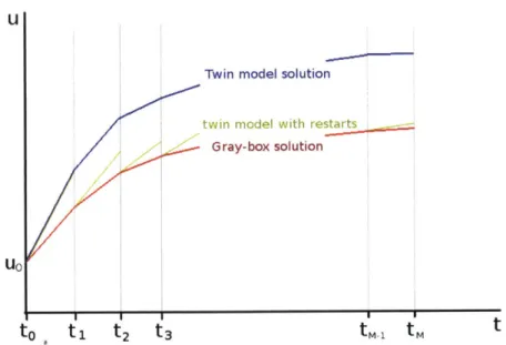
2-2 State-space trajectories of the gray-box model and the twin model. Mu measures the difference of the twin model trajectory (blue) with the gray-box trajectory (red). M, measures the difference of the twin model trajectory with restarts (green) and the gray-box trajectory (red). 53

2-3 An example mother wavelet, the Meyer wavelet. . . . . 56 2-4 Red line: the integral (2.19) of the Meyer wavelet. Black line: the

logistic sigmoid function. . . . . 58

2-5 An illustration of the tuple representation of univariate sigmoid functions. 59 2-6 The bases chosen manually for the numerical example of

Buckley-Leverett equation . . . . 60

2-7 The discretized gray-box solution is shuffled into three sets, each indicated by a color. Each block stands for the state variable on a space-time grid p oint. . . . . 61

2-8 (a) Gray-box solution used to train the twin model. (b) Trained twin-model solution by using the same initial condition as in the gray-box solution . . . . 63

2-9 (a) Gray-box model's flux F (red) and the trained twin-model flux P (blue). (b)

9

(red) and du (blue) . . . . 63 2-10 (a) Gray-box solution. (b) Out-of-sample solution of the trained twin

model by using the same initial condition as in (a). Because the domain of solution is contained in the domain of the training solution, the twin model and the gray-box model produce similar solutions. . . . . 64 2-11 (a) Gray-box solution. (b) Out-of-sample solution of the trained twin

model by using the same initial condition as in (a) . Because the domain of solution is beyond the domain of the training solution, a large deviation of the twin-model and gray-box solutions is observed. 64 2-12 Objective function evaluated by either the gray-box model and the

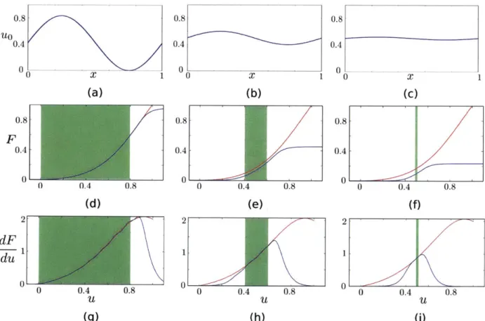
trained twin m odel. . . . . 65 2-13 (a,b,c) Three different initial conditions used to generate the gray-box

space-time solution. (d,e,f) compares the trained F (blue) and the Buckley-Leverett F (red). (g,h,i) compares the trained ! (blue) and the Buckley-Leverett -4E (red). The green background highlights the

domain of u where the gray-box space-time solution appears. . . . . . 66 2-14 Neighborhood for univariate bases. (a) Neighborhood (blue) of a single

basis (red). (b) Neighborhood (blue) of several bases (red). . . . . 70 2-15 The basis dictionary for the three solutions in Figure 2-13. The iteration

starts from the initial basis (1, 0). . . . . 75 2-16 The basis dictionary at each forward-backward iteration when the

initial condition is chosen as Figure 2-13c. In the left figure, the red dots indicate the bases in the dictionary, while the blue crosses indicate the deleted basis. In the right figure, the red line indicates the derivative of the true flux, while the blue line indicates the derivative of the trained flux. . . . . 78 2-17 Error of the estimated gradient, - , for the three solutions. The

2-18 Return bend geometry and the mesh for the simulation. The control points for the inner and outer boundaries are indicated by the red dots. 80 2-19 Left column: Example gray-box solution for a given geometry. Right

column: Solution mismatch after training a twin model. . . . . 83

2-20 The basis dictionary for the state equations, plotted on the

(

,

2) plane. The circles represent the bases that have ju = 1,

jO

= 1. The squares represent the bases that have ju = 2,

j,

= 1. The dots represent the bases that have ju = 2,

jI

= 2. . . . . 84 2-21 Cross-validation error M at each forward-backward iteration. The

y-axis is scaled by a constant, so that MT at the first forward-backward iteration equals 1. . . . . 84

2-22 State equation for the van der Waals gas, and for the Redlich-Kwong gas. Left column shows the trained state equation; right column shows the error of the state equation. The trained state equation is added by a constant, so the pressure matches the pressure of the gray-box equation at U = 2.6 and p = 0.7. The dashed red line shows the

convex hull of the gray-box solution. . . . . 85

2-23 Comparison of the estimated gradient and the true gradient for the Redlich-Kwong gas. The result for the van der Waals gas is visually indistinguishable to this plot. . . . . 86

2-24 Water flooding in petroleum reservoir engineering (from PetroWiki). Polymer solved in the water phase can be injected into the reservoir to enhance the production of oil. . . . . 87

2-25 The geometry of the petroleum reservoir. . . . . 89 2-26 The trained mobilities M, M., M.,. . . . . 90 2-27 Relative cross-validation error at each forward-backward iteration. The

x axis is the number of iteration, and the y axis is the integrated truncation error for MT of the three equations in (2.49). . . . . 92

2-28 Isosurfaces of S, = 0.25 and S, = 0.7 at t = 30 days. After the

2-29 Gradient of with respect to rates at the two injectors. The lines indicate the gradients estimated by the twin model, while the stars indicate the true gradient evaluated by finite difference. . . . . 94

3-1 Flowchart of Algorithm 3. . . . . 103 3-2 Optimized results for the Buckley-Leverett equation. . . . . 112 3-3 A comparison of the current best u(t = 1, x) after 20 gray-box simulations.

The red line is obtained by the vanilla Bayesian optimization and the green line by the twin-model Bayesian optimization. The cyan dashed line is the u(t = 1, x) obtained by setting the source term to zero. . . 112

3-4 The current best objective evaluation at each iteration. The red line is obtained by the Bayesian optimization without using the estimated gradient. The green line is obtained by using the estimated gradient. The black horizontal line indicates the true optimal, which is obtained

by BFGS using the true adjoint of the Buckley-Leverett equation. . . 113

3-5 (a) Initial guess of control points (blue dots); initial guess of the geometry (blue line); optimized control points (red dots); optimized geometry (red line) for the van der Waals gas. The blue squares indicate the bound constraints for each control point. (b) Pressure along the interior and the exterior boundaries for the initial (blue) and the optimized (red) geometry. (c) and (d) Results for the Redlich-K w ong gas. . . . . 115 3-6 Trained state equation, the error of the trained state equation, the

return bend geometry, and the basis dictionary at some iterations of the Bayesian optimization. The gray-box model uses the Redlich-Kwong state equation. The resolution of the bases is represented using the

3-7 Current best objective at each iteration for the van der Waals gas and the Redlich-Kwong gas. Green lines are obtained by the twin-model Bayesian optimization. Red lines are obtained by the Bayesian optimization without the estimated gradient. Black horizontal lines indicate the true optimal, obtained by BFGS using the true gradient. 120 3-8 Cumulative and per-iteration wall clock time, in minutes. Although

the twin-model Bayesian optimization is costlier per-iteration due to the training of twin model, it achieves near-optimality with less overall computational time. The gray-box model uses the Redlich-Kwong state equation . . . . 120 3-9 Permeability of the reservoir, in 100 milli Darcy. The five injectors are

indicated by the black dots, and the producer is indicated by the green

dot. ... ... 122

3-10 Current best objective evaluation against the number of iterates. The black line indicates the true optimal obtained by COBYLA optimization

[48],

a derivative-free optimization method. . . . . 123 3-11 (t) for the initial and the optimized injection rates. . . . . 123 3-12 Optimized time-dependent injection rates. . . . . 125 3-13 Current best objective evaluation using the backtracking-Armijo gradient

List of Tables

2.1 Error of the estimated gradients for the three solutions. The adaptively

constructed bases reduce the estimation error. . . . . 79

2.2 List of the dictionary for the van der Waals gas, (ju,

jP,

rIU, rP). ... 83

2.3 List of the dictionary for the Redlich-Kwong gas, (ju, Jp, lu, 7'/). . 83 2.4 Error of the gradient estimation, in percentage. . . . . 87

2.5 (jp, jsw, jc,rl,rsw, c) for M . . . . 89

2.6 (jp, jsw,jc, rp, r/sw, r7c) for Mwp . . . . 91

2.7 (jp, JswIc, /p, ?sw ,rc) for M w. . . . . 91

Nomenclature

* t E _{[0, T]: the time,}

" {ti}flm: the time steps, " x E Q: the space,

* {xj}_ 1: the spatial grid points,

* U: the space-time solution of gray-box conservation law,

" u: the space-time solution of twin-model conservation law,

" U: the discretized space-time solution of gray-box simulator,

" u: the discretized space-time solution of twin-model simulator,

" k: the number of equations of the conservation law; or the number of folds in cross validation.

" D: a known differential operator,

" F: the unknown function of the gray-box model, " P: the inferred F,

" q: the source term, " c: the control variables,

SC n = (cI, - -* , cn): _{a sequence of n control variables,}

" w: _{the quadrature weights in the numerical space-time integration,}

" : the objective function,

* t: the estimated gradient of with respect to c, * d: the number of control variables,

" C C Rd: the control space,

* K, G: the covariance functions,

" a: the acquisition function, "

M

: the solution mismatch,

*

M,:

the integrated truncation error,

* M: the mean solution mismatch in cross validation, "

#:

_{a basis function for F,}

"

j,

j: the dilation parameters of the basis for uni- and multi-variate functions,

" r/, r1: the translation parameters of the basis for uni- and multi-variate functions,

" A: the basis dictionary,

" a: the coefficients for

#,

" T: twin model,

" r: residual,

Chapter 1

Background

1.1

Motivation

A conservation law states that a particular property of a physical system does not appear or vanish as the system evolves over time, such as the conservation of mass, momentum, and energy. Mathematically, a conservation law can be expressed locally as a continuity equation (1.1),

F = q, (1.1)

(9t

where u is the conserved physical quantity, t is time, F is the flux that depends on u, and q is the source term that also depends on u. Many equations fundamental to the physical world, such as the Navier-Stokes equation, the Maxwell equation, and the porous medium transport equation, can be described by (1.1).

Optimization constrained by conservation laws is present in many engineering applications. For example, in gas turbines, the rotor blades can operate at a temperature close to 2000K

[10].

To prevent material failure due to overheating, channels can be forged inside the rotor blades to circulate coolant air whose dynamics are governed by the Navier-Stokes equation

[7].

The pressure used to drive the coolant flow is provided by the compressor, resulting in a penalty on the turbine's thermo-dynamic efficiency

[8].

Engineers are thereby interested in optimizing the coolant channel geometry in order to suppress the pressure loss. In this optimization problem, the control variables are the parameters that describe the channel geometry. The dimensionality of the optimization is the number of control variables, i.e., the control's degree of freedom. Another example is the field control of petroleum reservoir. In the petroleum reservoir, the fluid flow of various phases and chemical components is dictated by porous medium transport equations

[4].

The flow can be passively and actively controlled by a variety of techniques

[1],

such as the wellbore pressure control, the polymer injection, and the steam heating [5]. The pressure, injection rate, and temperature can vary in each well and during every day over decades of continuous operations. The dimensionality of the optimization is the total number of these control variables. Driven by economic interests, petroleum producers are devoted to optimizing the controls for enhanced recovery and reduced cost.

Such optimization has been revolutionized by the numerical simulation and optimization algorithms. On the one hand, conservation law simulation can provide an evaluation of a candidate control that is cheaper, faster, and more scalable than conducting physical experiments. On the other hand, advanced optimization algorithms can guide the control toward the optimal with reduced number of simulation 140, 41, 42, 50, 54, 55, 56, 72]. However, optimization based on conservation law simulation can still be overwhelmingly costly. The cost is two-fold: First, each simulation at a given control may run for hours or days even on a high-end computer. Such expense in time is usually a result of using high-fidelity physical models, complex numerical schemes, and large-scale space-time discretization schemes. Second, optimization algorithms generally take many iterations of simulation on various controls. The number of iterations required to achieve near-optimality usually increases with the control variables' degree of freedom [601. The two costs are multiplicative. The multiplicative effect compromises the impact of computational efforts among field engineers.

Fortunately, the cost due to iteration can be alleviated by adopting gradient-based optimization algorithms [60]. A gradient-based algorithm requires significantly fewer iterations than a derivative-free algorithm for problems with many control variables

[19,

60, 41]. Gradient-based algorithms require the gradient of the optimization objective to the control variables, which is efficiently computable through the adjoint method [11]. The adjoint method propagates the gradient from the objective backward to the control variables through the path of time integration [11] or the chain of numerical operations [18]. To keep track of the back propagation, the simulator source code needs to be available. However, many industrial simulators do not have the adjoint capability because their codes were developed without the adjoint technique in mind. The implementation of the adjoint method in these legacy simulators can be a major undertaking. For example, PSim, a reservoir simulator developed and owned by ConocoPhillips, is a multi-million-line Fortran-77 code that traces its birth back to the 1980's. Implementing adjoint directly into the source code is not preferable because it can take a tremendous amount of brain hours. Besides, the source code and its physical models are only accessible and modifiable by the computational team inside the company. For the sake of gradient computation, PSim has been superseded by adjoint-enabled simulators, but it is hard to be replaced due to its legacy usage. The legacy nature of many industrial simulators hinders the prevalence of the adjoint method and gradient-based algorithms in many real-world problems with high-dimensional control.

Despite their legacy nature, most simulators for unsteady conservation laws can provide the discretized space-time solution of relevant flow quantities. For example,

PSim provides the space-time solution of pressure, saturation, and concentration for

multi-phase flow. Similarly, most steady-state simulators can provide the spatial solution. Thus, the discussion will focus on the unsteady case because a steady-state simulator can be viewed as a special case of unsteady-state simulators where the solutions remain the same over many time steps.

My thesis considers the conservation laws whose flux functions have an unknown algebraic dependence on the state variables. The adjoint gradient computation may be enabled by leveraging the space-time solution. The discretized space-time solution provides invaluable information about the conservation law hardwired in the simulator. For illustration, consider a code that simulates

+u = , _{E [0,1], tE [0,1] (1.2)}

a

t

ax

with proper initial and boundary conditions and F being differentiable. c indicates the control that acts as a source for u. If the expression of F(u) in the simulator is not accessible by the user, adjoint can not be implemented directly. However,

F may be partially inferred from a discretized space-time solution of u for a given

c. To see this, let the discretized solution be u = {u(ti,xj)}i=1,..,M, j=1,..-,N, where 0 < ti < t2 < ... < t < I and 0 < x, < 2 < ... < xN < I indicate the time

and space discretization. Given u, the a and u can be sampled by finite difference. Because (1.2) can be written as

Du d Fu _

+ = C , X E [0, 1] , t C [0, 1] (1.3)

at du ax

away from the shock wave, the samples of a and 2 can be plugged into (1.3) to obtain samples of !. The reasoning remains intact at the shock wave, where ! in

(1.3) is replaced by the finite difference form 2 according to the Rankine-Hugoniot condition. Based upon the sampled ! and 4, the unknown flux function F can be approximated up to a constant for values of a that appeared in the solution, by using indefinite integral. Let P be the approximation for F. An alternative conservation law can be proposed

a

c, E _{[0,1], tE [0,1], (1.4)}

at

ax

that approximates the true but unknown conservation law (1.2), where ii is the solution associated with P, in the following sense: If F and F are off by a constant

a, i.e. F = F + a, then dFTu) _du = d(F(u)+a) _du dFu); _du therefore, the solutions of (1.2) and (1.4) to any initial value problem will be the same. The gradient of any objective function c(c) = (u(c), c) can be obtained by the adjoint method

[11].

The gradient is

< _{+ A dxdt , (1.5)}

where A, the adjoint solution, satisfies

aAa(AdF>8

A+ a =F- a . (1.6)

at ax du au

In (1.6), L and 2 are defined on the solution u of (1.3) [11]. Similarly, the gradient of (c) (i(c), c) is

-- = _{-- +} ( dxdt , (1.7)

dc 0 0 ac

where

A,

the adjoint solution, satisfies

a a dF a

at

x

du

Ou(

In (1.8), d and L are defined on the solution ft of (1.4). If the two solutions, u and f, are the same, and if d =dF on the solution, then the adjoint solutions, A and A will be the same. As a result, the gradients, (1.5) and (1.7), will be the same. Therefore can drive the optimization constrained by (1.2). A simulator for the approximated conservation law is named "twin model" because it behaves as an adjoint-enabled twin of the original simulator. If a conservation law has a system of equations and/or has a greater-than-one spatial dimension, the above simple method to recover the flux function from a solution will no longer work. Nonetheless, much information about the flux function can be extracted from the solution. Given some additional information of the conservation law, one may be able to recover the unknown aspects of the flux function. The details of this topic are discussed in Chapter 2.

1. The adjoint is unavailable, and the adjoint is impractical to be implemented into the source code.

2. The full space-time solution of relevant flow quantities is available.

My thesis considers gray-box simulators whose flux functions contain unknown algebraic dependence on the state, and whose boundary conditions, initial conditions, source terms, and differential operators in the flux functions are known. For example, a Navier-Stokes flow simulation can have an unknown state equation; in other words, the pressure term contains an unknown algebraic dependence on the state. Another example is a reservoir simulation whose phase velocities are governed by Darcy's law

[4], which can contain unknown algebraic dependence on the phases' saturations. In

contrast, a simulator is named open-box if condition one is violated. For example,

OpenFOAM

1611

is an open-source fluid simulator where adjoint can be implemented directly into its source code, so it is open-box by definition. Open-box simulators enjoy the benefit of efficient gradient computation brought by adjoint and thereby are not within the research scope of my thesis. If condition one is met, but two is violated, a simulator is named "black-box". For example, Aspen [621, an industrial chemical reactor simulator, provides neither the adjoint nor the full space-time solution. Black-box simulators are simply calculators for the objective function. Due to the lack of space-time solution, adjoint can not be enabled using the twin model. Gray-box simulators are ubiquitous in many engineering applications. Examples are Fluent [106] and CFX [107] for computational fluid dynamics, and ECLIPSE (Schlumberger), PSim (ConocoPhillips), and MORES (Shell) for petroleum reservoir simulations. My thesis will only investigate gray-box simulators.

My thesis aims at reducing the number of expensive iterations in the optimization constrained by gray-box simulators. Motivated by the adjoint gradient computation, a mathematical procedure will be developed to estimate the adjoint gradient by leveraging the full space-time solution. Also, my thesis will investigate how the estimated gradient can facilitate a suitable optimization algorithm to reduce the

number of iterations. Finally, the iteration reduction achieved by my approach will be assessed, especially for problems with many control parameters.

Instead of discussing gray-box simulators in general, my thesis only focuses on simulators with partially unknown flux function, while their boundary condition, initial condition, and the source term are known. For example, one may know that the flux depends on certain variables, but the specific function form of such dependence is unknown. This assumption is valid for some applications, such as simulating a petroleum reservoir with polymer injection. The flow in such reservoir is governed by multiphase multicomponent porous medium transport equations

[4].

The initial condition is usually given at the equilibrium state, the boundary is usually described by a no-flux condition, and the source term can be modeled as controls with given flow rate or wellbore pressure. Usually, the flux function is given by Darcy's law which involves physical models like the permeability and the viscosity2. The mechanism through which the injected polymer modifies the rock permeability and flow viscosity can be unavailable. Thereby the flux is partially unknown. The specific form of PDE considered in my thesis is given in Section 1.2. It is a future work to extend my research to more general gray-box settings where the initial condition, boundary condition, source term, and the flux are jointly unknown.

1.2

Problem Formulation

Consider the optimization problem

c* argmax (u, c)

Cmin C Cmax

M N T1-9)

(C) = Y, wij

f(Ui,

c; ti, X) j f(u C; t, X)dxdt i=1 j=1

'The permeability quantifies the easiness of liquids to pass through the rock.

where u and u are the discretized and continuous space-time solutions of a gray-box conservation law simulator. u and u depend on the control variables c. We assume to be a twice differentiable function. The spatial coordinate is x E Q and the time is

t E [0, T]. i = 1, . . , M and

j

= 1, - - - , N are the indices for the time and space grid

points.

f

is a given function that depends on u, c, t, and x. wij's are the quadrature weights for the integration. c E Rd indicates the control variable. cmin and cmax are elementwise bound constraints.

The gray-box simulator solves the partial differential equation (PDE)

au + V - (DF(u)) = q(u, c), (1.10)

at

which is a system of k equations. The initial and boundary conditions are known. D is a known differential operator that may depend on u, and F is an unknown function. Although the state variables that F depend on are known, the algebraic form of such dependence is unknown. q is a known source term that depends on u and

c. The simulator for (1.10) does not have the adjoint capability, and it is infeasible to

implement the adjoint method into its source code. But the full space-time solution u is provided. The steady-state conservation law is a special case of the unsteady one, so it will not be discussed separately.

For example, consider a 1-D scalar-state convective equation

+ aF(u) = c, (1.11)

can be described by (1.10). The flux function F is known to depend on the local value of the state variable u, but the algebraic form of the dependence is unknown. In this case, F represents the entire unknown flux function while D equals 1. If

F(u) =

jIu2,

(1.11) is the Burger's equation; If F(u) = U) (1.11) is a

Another example can be the compressible, viscous, adiabatic Navier-Stokes equation

p pu Pv

9 p( '

PU2 ₊

p -u7X

+

PUV

-

oPy _Pu

Li xx=0,

at

P

ax

PUVaxy _{ay PV} 2 +P - O-yy

pE u(Ep + p) - axuu- OXYv v(Ep+ p) - oxyu - oryvj

(1.12) where

au

2

(au

av

Oa=pt 2 --- _+ ax 3 ax ay)

av

2 Ou

av

O-yy =p2 + . (1.13) ay 3 ax ay)

(au

av

a

ax)J

Let p, u, v, E, U, and p be the density, Cartesian velocity components, total energy, internal energy, and pressure. The pressure depends on the density and energy, but the algebraic form of the dependence is unknown. In this example, F(u) corresponds to the pressure equation p = p(p, U), and D corresponds to the known components of the flux functions.

My thesis does not accomodate the PDEs that contain unknown source terms or flux functions with unknown differential operators, thus limiting the applicability of my thesis. It is a future research topic to extend the methods developed in this thesis for such PDEs.

My thesis focuses on reducing the number of gray-box simulations in the optimization, especially for problems where d, the dimensionality of the control variable, is large. I

assume that the computational cost is dominated by the repeated gray-box simulation, while the cost of the optimization algorithm is relatively small. Chapter 2 develops a mathematical procedure, called the twin-model method, which enables adjoint

gradient computation by leveraging the full space-time solution. Based on previous research [66, 67, 71, 72, 74, 76, 77], Chapter 3 develops an optimization algorithm that takes advantage of the estimated gradient to achieve iteration reduction. The utility of the estimated gradient for optimization is analyzed both numerically and theoretically.

1.3

Literature Review

Given the background, I review the literature on derivative-free optimization and gradient-based optimization, in which the Bayesian optimization method is particularly investigated. In addition, I review the adjoint method because it is an essential ingredient for Chapter 2. Finally, I review methods for adaptive basis construction, which is useful for the adaptive parameterization of a twin model.

1.3.1

Review of Optimization Methods

Optimization methods can be categorized into derivative-free and gradient-based methods [41], depending on whether the gradient information is used. In this section, I review the two types of methods.

Derivative-Free Optimization

Derivative-free optimization (DFO) requires only the availability of objective function values but no gradient information

[411;

thus, it is useful when the gradient is unavailable,

unreliable, or too expensive to obtain. Such methods are suitable for problems constrained by black-box simulators.

Depending on whether a local or global optimum is desired, DFO methods can be categorized into local methods and global methods

[411.

Local methods seek a local optimum which is also the global optimum for convex problems. A local method is the derivative-free trust-region method [47]. The derivative-free trust-region method

introduces a surrogate model that interpolates the objective evaluations [48, 51]. The surrogate model is cheap to evaluate and presumably accurate within a trust region: an adaptive neighborhood around the current iteration [46, 47]. At each iteration, the surrogate is optimized in a domain bounded by the trust region to generate candidate steps for additional objective evaluations [46, 471.

Global methods seek the global optimum. Example methods include the branch-and-bound search [521, evolution methods [53], and Bayesian methods [71, 73, 911. The branch-and-bound search sequentially partitions the entire control space into a tree structure and determines lower and upper bounds for the optimum [52]. Partitions that are inferior are eliminated in the course of the search [52]. The bounds are usually obtained through the assumption of the Lipschitz continuity or statistical bounds for the objective function [52]. Evolution methods maintain a population of candidate controls, which adapt and mutate in a way that resembles natural phenomenons such as natural selection [54, 56] and swarm intelligence

[55].

Bayesian methods model the objective function as a random member function from a stochastic process. At each iteration, the statistics of the stochastic process are calculated and the posterior, a probability measure, of the objective, is updated using Bayesian metrics [71, 72]. The posterior is used to pick the next candidate step that best balances the exploration of unsampled regions and the exploitation around the sampled optimum [73, 82, 69]. Details of Bayesian optimization methods are discussed in Section 1.3.1.

Because many real-world problems are non-convex, global methods are usually preferred to local methods if the global optimum is desired [41]. Besides, DFO methods usually require a large number of function evaluations to converge, especially when the dimension of control is large

[411.

This issue can be alleviated by incorporating the gradient information

[66,

74]. The details are discussed in the next subsection.

Gradient-Based Optimization

Gradient-based optimization (GBO) requires the availability of the gradient values [60, 83]. A gradient value, if it exists, provides the optimal infinitesimal change of control variables at each iterate and thus is useful in searching for better control. Similar to DFO, GBO also can be categorized into local methods and global methods [60]. Examples of local GBO methods include the gradient descent methods [84,

1041, the conjugate gradient methods

[85,

86], and the quasi-Newton methods

[40,

42]. The gradient descent methods and the conjugate gradient methods choose the search step in the direction of either the gradient [84, 104] or a conjugate gradient [85, 86]. Quasi-Newton methods, such as the Broyden-Fletcher-Goldfarb-Shannon (BFGS) method

[40],

approximate the Hessian matrix using a series of gradient values. The approximated Hessian allows a local quadratic approximation to the objective function, which determines the search direction and stepsize by the Newton's method [40]. In addition, some local DFO methods can be enhanced to use gradient information [58, 59]. For instance, in trust-region methods, the construction of local surrogates can incorporate gradient values if available [58, 59]. The usage of a gradient usually improves the surrogate's accuracy, thus enhancing the quality of the search step and thereby reducing the required number of iterations [58, 59].

Global GBO methods search for the global optimum using gradient values [60, 83]. Some global GBO methods can trace their development to corresponding DFO methods. For example, the stochastic gradient-based global optimization method (StoGo) [87, 88] works by partitioning the control space and bounding the optimum in the same way as the branch-and-bound method

[52].

But the search in each partition is performed by gradient-based algorithms such as BFGS [40].

My thesis is particularly interested in the gradient-based Bayesian optimization method

[75].

In this method, the posterior of the objective function assimilates both the gradient and function values in a CoKriging framework [66, 75]. The details of

my treatment are discussed in Section 1.3.1 and Chapter 3. It is reasonable to expect that the inclusion of gradient values results in a more accurate posterior mean and reduced posterior uncertainty, which in turn reduces the number of iterations required to achieve near-optimality. The effect of iteration reduction is analyzed numerically in Chapter 3.

A property of the Bayesian method is that the search step can be determined using all available objective and gradient values [71, 82]. Also, given the current knowledge of the objective function which is represented in Bayesian probability, the search step is optimal under a particular metric such as the expected improvement metric [71, 82]. The advantage of such properties can be justified when the objective and gradient evaluations are dominantly more expensive than the overhead of optimization algorithm

[71].

Besides, my thesis proves that the Bayesian optimization method is convergent even if the gradient values are estimated inexactly, which is discussed in Section 3.3. The conclusion of Section 3.3 reveals that, under some assumptions of the objective and the inexact gradient, a Bayesian optimization algorithm can find the optimum regardless of the accuracy of the gradient estimation.

To achieve the desired objective valuation, GBO methods generally require fewer iterations than DFO methods for problems with many control variables

[60,

83]. GBO methods can be efficiently applied to optimization constrained by open-box simulators because the gradient is efficiently computable by the adjoint method [11, 60], which is introduced in the next subsection. My thesis extends GBO to optimization constrained by gray-box simulation by estimating the gradient using the full space-time solution.

Bayesian Optimization

Similar to other kinds of optimization, Bayesian optimization aims at finding the maximum of a function

(-)

in a bounded set C C Rd

[71,

72, 82]. However, Bayesian optimization distinguishes from other methods by maintaining a probabilistic model

for [71, 72, 82]. The probabilistic model is exploited to make decisions about where to invest the next function evaluation in C [71, 72, 82]. In addition, it uses all information of available evaluations, not just local evaluations, to direct the search step [71, 72, 82].

Consider the case when the objective function evaluation is available. Bayesian optimization begins by assuming that the objective function is sampled from a stochastic process [71, 72, 82]. A stochastic process is a function

f : C x Q+R ,(1.14)

(c,w) - f(c, w)

where for any c E C. w is a random variable that models the stochastic dependence of f. f(c, -) is a random variable defined on the probability space (Q, E, P). The

objective function is assumed to be a sampled function from the stochastic process

(-)

= f(-, w*), where w* E Q is deterministic but unknown. My thesis will use the notations

(-),

f(., w), and f(-, w*) interchangeably when the context is clear.

A stationary Gaussian process is a type of stochastic process that is used ubiquitously in Bayesian optimization [89]. For any given w and any finite set of N points

{ci

E C} 1, a stationary Gaussian process f(-,-) has the property that

{f

(ci, -)}_ are

multivariate Gaussian distributed; in addition, the distribution remains unchanged if ci's are all added by the same constant in C. The Gaussian process is solely determined by its mean function m(c) and its covariance function K(c, c') [89]

m(c) = E [f (c, w)]

K(c, c') = E [(f (c, W) - m(c)) (f (c', w) - m(c'))]

for any c, c' E C, which is denoted by f ~ K(m, K). Conditioned on a set of

and covariance

[89]

ni(c) = m(c) + K(c, c)K(c, c.)-1 ( (cf) - m(cf)) (1.16)

k(c,

c') = K(c, c') - K(c, c,)K(c., c)--K(cf, c') where c, (ci, - --, CN), (C) = ((cl), - - - , (CN) )T, m(c) = (m(C), - ,m(CN) )T K(c, cf) = K(cn, c)T = (K(c, cl), -.- , K(c, CN)), and K(ci, cl) ... K(ci, CN) K(c.,c.) =

I-.

K(CN, C1) ... K(CN, CN)

Without prior knowledge about the underlying function, m(.) is usually modeled as a constant independent of c [89]. In many cases, the covariance are assumed isotropic, indicating that K(c, c') only depends on the L2 norm 1|c - c'|| [89]. There are many

choices for K, such as the exponential kernel, the squared exponential kernel, and the Matern kernels, each embeds different degrees of smoothness (differentiability) for the underlying function. For a survey of various covariance functions, I refer to the Chapter 4 in [89]. Among such choices, the Matern 5/2 kernel [90]

(

\/'c -

c'II

5|Ic

-

c'' 2'5||c

-c'H'

K(c, c') = .

1

+ L + 3L2 exp

K

L ' (1.17)

has been recommended because it results in functions that are twice differentiable, an assumption made by, e.g. quasi-Newton methods, but without further smoothness

[71]. My thesis will focus on using the Matern 5/2 kernel. Notice the parameters

L and -, known as the hyperparameters, are yet to be determined. They can be determined by the posterior maximum likelihood estimation (MLE) or by a fully-Bayesian approach [71, 82]. I refer to the reference [711 for the details and a comparison of these treatments. My thesis will focus on MLE due to its simpler numerical

Based on the posterior and the current best evaluation Cbest = argmaxcEc (c),

Bayesian optimization introduces an acquisition function, a : C R+, which evaluates the expected utility of investing the next sample at c E C [69, 71, 72, 82, 91]. The location of the next sample is determined by an optimization CN+1 = argmaxcEC a(c)

[69, 71, 72, 82, 91]. In most cases, a greedy acquisition function is used, which evaluates the one-step-lookahead utility [69, 71, 72, 82, 91]. There are several choices for the acquisition function, such as

* the probability of improvement (PI) [91],

apI(c) = P(y(c)), (1.18)

* the expected improvement (EI) [72, 731,

aEI (C) = u(c)(y(c)<(y(c)) +A(y(c))) , (1.19)

" and the upper confidence bound (UCB) [69],

aUCB(C) = A(C) + KU(c) , (1.20)

with a tunable parameter r > 0,

where p, u are the posterior mean and variance, -y(c) = -- (c) (Pi(c) - (Cbest)),

and 41,V indicate the cumulative and density functions for the standard normal distribution. My thesis will focus on the El acquisition function, as it behaves better than the PI and requires no extra tunable parameters [71]. Because (1.19) has a closed-form gradient, the acquisition function can be maximized by a global GBO method, e.g., StoGo [88], to obtain its global maximum.

Although my thesis only focuses on bound constraints as shown in (1.9), Bayesian optimization can accommodate more general inequality and equality constraints [97]. The constraints can be enforced by modifying the objective, such as the penalty

method [921, the augmented Lagrangian method [93], and the barrier function method [94]. They also can be enforced by modifying the acquisition function, such as the recently developed expected improvement with constraints (EIC) method

[95],

and the integrated expected conditional improvement (IECI) method

[96].

See Chapter 2 of

[97]

for a detailed review of constrained Bayesian optimization.

In addition to function evaluations

(c),

Bayesian optimization admits gradient information [66, 74]. In Chapter 3, I investigate the scenario where the gradient evaluations are inexact

[77].

The Bayesian optimization method developed in my thesis allows both the exact function evaluation and the inexact gradient evaluation.

1.3.2

The Adjoint Method

Consider a differentiable objective function constrained by a conservation law PDE (1.10). Let the objective function be (u, c), c E Rd, and let the PDE (1.10) be abstracted as F(u, c) = 0. F is a parameterized differential operator, together with boundary conditions and/or initial conditions, which uniquely define a u for each c. The gradient / can be estimated trivially by finite difference. The ith component of_dc the gradient is given by

- ~~ -(WU + Aui, C + 6ei) -((U, 6)) (1.21)

dc) i 6

where

Y(u, c) = 0, E(u +AUi, C + 6ei) = 0. (1.22)

ei indicates the ith unit Cartesian basis vector in R d, and 6 > 0 indicates a small perturbation. Because (1.22) needs to be solved for every 6ei, so that the corresponding

Au, can be used in (1.21), d+1 PDE simulations are required to evaluate the gradient.

Therefore, it can be costly to evaluate the gradient by finite difference.

In contrast, the adjoint method evaluates the gradient using only one PDE simulation plus one adjoint simulation [11]. To see this, linearize F(u, c) = 0 into a variational form 6F= u + -6c = 0, (1.23) au ac which gives -- = - -

-

(1.24) dc Ou ac

Using (1.24), 9 can be expressed by

d _ du a

dc audc ac

-1

0c &(1.25)

-AT a + a

Dc Dc

where A, the adjoint state, is given by the adjoint equation

A_ = ( (1.26)

au au

Therefore, the gradient can be evaluated by (1.25) using one simulation of F(u, c) = 0 and one simulation of (1.26) that solves for A.

Adjoint methods can be categorized into continuous adjoint and discrete adjoint methods, depending on whether the linearization or the discretization is executed first [15]. The above procedure, (1.23) through (1.26), is the continuous adjoint, where F is a differential operator. The continuous adjoint method linearizes the continuous PDE F(u, c) = _{0 first and then discretizes the adjoint equation (1.26) [11]. In (1.26),}

) can be derived as another differential operator. With proper boundary and/or initial conditions, it uniquely determines the adjoint solution A. See [19] for a detailed derivation of the continuous adjoint equation.

. The discrete adjoint method

[17]

discretizes F(u, c) = 0 first. After the discretization,

u and c become vectors u and c. u is defined implicitly by the system Yd(u, c) = 0,

where T_{d indicates the discretized difference operator, a nonlinear function whose} output is of the same dimension as its first input u. Using the same derivation as (1.23) through (1.26), the discrete adjoint equation can be obtained

X = (,,) )(1.27)

au Tu '

which is a linear system of equations. (.d

)T

is derived as another difference operator which is a square matrix. It contains the discretized boundary and initial conditions, and uniquely determines the discrete adjoint vector A, which subsequently determines the gradient

S-A + . _(1.28)

dc ac ac

See Chapter 1 of [20] for a detailed derivation of the discrete adjoint.

The adjoint method has seen wide applications in optimization problems constrained by conservation law simulations, such as in airfoil design [12, 13, 14], adaptive mesh refinement [20], injection policy optimization in petroleum reservoirs

[2],

history matching in reservoir geophysics [15], and optimal well placement in reservoir management [16].

1.3.3 Adaptive Basis Construction

The unknown function F in (1.10) can be approximated by a linear combination of basis functions

[241.

An over-complete or incomplete set of bases can negatively affect the approximation due to overfitting or underfitting

[25].

Therefore, adaptive basis construction is needed.

Consider the problem of function approximation in a bounded domain. Square-integrable functions can be represented by the linear combination of a set of basis functions

[24],

{#i}iEN, such as the polynomial basis, Fourier basis, and the wavelet basis [102].

F(.) = aii(-) , _(1.29)

iEN

where

#j's

are linearly independent basis functions, ai's are the coefficients, and i indices the basis. For a rigorous development of function approximation and basis functions, I refer to the book [24].

For example, a bivariate function can be represented by monomials (Weierstrass approximation theorem [105])

1, u1, uf, u2 U2l2, U 2 U , , 21U , U

-on any real interval [a, b].

Let A be a finite non-empty subset of N, F can be approximated using a subset of bases,

F(.) ~ aiq0(i), (1.30)

iEA

where {i}ieA is called a basis dictionary [31]. The approximation is solely determined by the choices of the dictionary and the coefficients. For example, in polynomial approximation, the basis dictionary can consist of the basis whose total polynomial degree does not exceed p E N [26]. Given a dictionary, the coefficients for F can be determined by the minimization [26]

Ci* = argmin - i , (1.31)

aERIAI _iGA

where 11 - |IL indicates the Lp norm3_{. My thesis parameterizes the twin-model flux}

P and optimizes the coefficients, so the twin model serves as a proxy of the gray-box model. The details are discussed in Section 2.2.

If the dictionary is pre-determined, its cardinality can increase as the number of variables increases, and as the basis complexity increases [26]. For example, for the d-variate polynomial basis, the total number of bases is dP if one bounds the polynomial

degree of each variable by p; and is (Pd) if one bounds the total degree by p [26].

In many applications, one may deliver a similarly accurate approximation by using a much smaller subset of the dictionary as the bases than using all the basis functions in the dictionary [26, 28, 31, 44]. To exploit the sparse structure, only significant bases shall be selected, and the selection process shall be adaptive depending on the values of function evaluations. There are several methods that adaptively determine the sparsity, such as Lasso regularization

[44],

matching pursuit [31], and basis pursuit [28]. Lasso regularization adds a penalty A E Iai I to the approximation error, where A > 0 is a tunable parameter [44]. The larger A is, the sparser the basis functions will be. In this way, Lasso balances the approximation error and the number of non-zero coefficients [44]. Matching pursuit adopts a greedy, stepwise approach [31]. It either selects a significant basis one at a time (forward selection) from a dictionary [32], or prunes an insignificant basis one at a time (backward pruning) from the dictionary [33]. Basis pursuit minimizes

||cHL,

subject to (1.29), which is equivalently reformulated and efficiently solved as a linear programming problem [28].

Conventionally, the dictionary for the sparse approximation needs to be predetermined, with the belief that the dictionary is a superset of the required bases for an accurate approximation

[35].

This can be problematic because the required bases are unknown a priori. To address this issue, methods have been devised that construct an adaptive dictionary [34, 35, 36]. Although different in details, such methods share the same

approach: In the beginning, some trivial bases are given as inputs. For example, the starting basis can be 1 for a polynomial basis

[341.

The starting bases serve as seeds from which more complex bases grow. I refer to [34, 35, 361 for more details of the heuristics. Then a dictionary is built up progressively by iterating over a forward step and a backward step [34, 35, 36]. The forward step searches over a candidate set of bases and appends the significant ones to the dictionary [34, 35, 361. The backward step searches over the current dictionary and removes the insignificant ones from the dictionary [34, 35, 36]. The iteration stops only when no alternation is made to the dictionary or when a targeted accuracy is achieved, without bounding the basis complexity a prior [34, 35, 36]. Such approach is adopted in my thesis to build up the bases for P. The details are discussed in Section 2.3.

1.4

Thesis Objectives

Based on the motivation and literature review, we find it useful to enable adjoint gradient computation for gray-box conservation law simulations whose flux functions have an unknown algebraic dependence on the state variables. We also need to exploit the estimated gradient to optimize more efficiently, especially for problems with many control variables. To summarize, the objectives of my thesis are

1. to develop an adjoint approach that estimates the gradient of objective functions constrained by gray-box conservation law simulations with unknown algebraic dependence in the flux functions, by leveraging the space-time solution;

2. to assess the utility of the estimated gradient in a suitable gradient-based optimization method; and

3. to demonstrate the effectiveness of the developed procedure in several numerical examples, given a limited computational budget.